An efficient approximation method for calculating confidence level of negative survey

(1)

Research Article

An Efficient Approximation Method for Calculating

Confidence Level of Negative Survey

Ran Liu, Jinghui Peng, and Shanyu Tang

School of Computer Science, China University of Geosciences, Wuhan, China

Correspondence should be addressed to Shanyu Tang; [email protected]

Received 27 April 2015; Revised 23 July 2015; Accepted 2 September 2015

Academic Editor: Ofer Hadar

Copyright © 2015 Ran Liu et al. This is an open access article distributed under the Creative Commons Attribution License, which permits unrestricted use, distribution, and reproduction in any medium, provided the original work is properly cited.

The confidence level of negative survey is one of the key scientific problems. The present work uses generation function to analyse the confidence level and uses a greedy algorithm to calculate that, which is used to evaluate the dependable level of negative survey. However, the present method is of low efficiency and complex. This study focuses on an efficient approximation method for calculating the confidence level of negative survey. This approximation method based on central limit theorem and Bayesian method can get the results efficiently.

1. Introduction

Artificial immune system simulates the mechanism of biol-ogy immune system to model and design effective algorithm for solving some complex issues. Negative selection principle [1] is one of the unique mechanisms of biology immune system, and the implication of negative selection principle is that the immaturity T cell dies if itmatcheswith itself as it grows, and it survives if itmismatcheswith itself. Inspired by negative selection principle, the negative selection algorithm [2] is proposed and can be used for network security, virus detection [3, 4], and anomaly detection [5].

Similarly, the negative survey [6], which is inspired by negative selection principle, is a novel and promising indirect question method for information security and enhancing privacy in collecting sensitive data and individual privacy [7]. Negative surveys consist of a question and𝑐 (𝑐 ≥ 3)categories for the interviewees to select from. In contrast to traditional surveys, the participants are required to select a category that doesnot agree with the fact [6, 8]; that is, randomly select a category from the other𝑐 − 1unreal categories. For convenience, it definespositive categoryas the category that agrees with the fact, while it definesnegative categoryas the other𝑐 − 1categories that donotagree with the fact [6].

The negative survey method can attain privacy protection with lower power and higher degree and boost participants’ confidence. The main calculation of collecting sensitive data

with negative survey is reconstructing the corresponding positive survey in the central processor. The privacy preserv-ing properties of negative survey do not rely on anonymity, cryptography, or any legal contracts, but rather participants not revealing their own privacy information. And the nega-tive survey method is applicable to collecting data at a high speed in low-powered mobile devices such as smart phones and tablets [9].

The positive survey can be reconstructed from a result of negative survey. For a survey consisting of a question

and𝑐 (𝑐 ≥ 3) categories for𝑛interviewees to select from,

a negative survey result is 𝑅 = (𝑟₁, 𝑟₂, . . . , 𝑟_𝑐), where 𝑟_𝑖 is the results of category𝑖in negative survey. Meanwhile, the original positive survey is 𝑇 = (𝑡₁, 𝑡₂, . . . , 𝑡_𝑐), where 𝑡_𝑖 is the number of interviewees belonging to category𝑖. Define V_𝑖,𝑗as the probability that category𝑖is chosen given that a respondent positively belongs to category𝑗, where∑𝑐_𝑖=1V_𝑖,𝑗=

1andV_𝑖,𝑖 = 0. Define the probability matrix as𝑉as Formula (1), and𝑅 = 𝑇𝑉and𝑇 = 𝑅𝑉−1. In consequence, the positive survey𝑇can be reconstructed from a negative survey𝑅:

𝑉 = [ [ [ [ [ [ [

0 V1,2 ⋅ ⋅ ⋅ V1,𝑐 V_2,1 0 ⋅ ⋅ ⋅ V_2,𝑐

... ... d ...

V𝑐,1 V𝑐,2 ⋅ ⋅ ⋅ 0 ] ] ] ] ] ] ]

. (1)

(2)

Generally,V𝑖,𝑗|𝑖 ̸=𝑗= 1/(𝑐−1), which means the probability of selecting negative categories follows uniform distribution [6]. Following the work in [6], Xie et al. proposed Gaus-sian Negative Survey (GNS) [10], where the probabilities of selecting negative categories (i.e.,V𝑖,𝑗) follow a Gaussian distribution centered at the corresponding positive category. The GNS could attain higher accuracy but lower ability of privacy protection.

The traditional reconstructing method in [6] may lead to the reconstruction of positive survey with negative values. Based on the problem, two methods [11] were proposed for reconstructing positive survey which had no negative values. In [12], Bao et al. proposed a greedy algorithm for calculating the confidence level, which is analysed in generating function. But this method is of low efficiency and complex and could not achieve the high efficiency of negative survey.

In this study, an efficient approximation method is pro-posed to calculate the confidence level of negative survey. This work reinforces the efficiency of negative survey.

In the remainder of this study, Section 2 introduces the related work of this study. Section 3 describes the problem in this study. Section 4 describes the efficient approximation method. Section 6 discusses some existing problems of this approximation method and Section 7 concludes the whole study.

2. Related Work

In this study, the probability of selecting negative categories follows uniform distribution (i.e., V𝑖,𝑗|𝑖 ̸=𝑗 = 1/(𝑐 − 1)) as general negative survey in [6, 8, 11, 12]. So, in this section, the related work of negative survey [6, 8, 11, 12] is introduced. For convenience, some definitions are given in the followoing list:

𝑛: the number of interviewees for surveys.

𝑐: the number of categories in surveys.

𝑟𝑖: the number of interviewees selecting category𝑖in negative survey.

𝑞_𝑖: the proportion of negative category𝑖 (1 ≤ 𝑖 ≤ 𝑐); that is,𝑞_𝑖= 𝑟_𝑖/𝑛.

𝑡𝑖: the original number of interviewees in positive category𝑖.

̂𝑡𝑖: the estimated number of𝑡𝑖.

𝑅: the participant vector; that is,𝑅 = (𝑟₁, 𝑟₂, . . . , 𝑟_𝑐).

𝑇: the participant vector; that is,𝑇 = (𝑡₁, 𝑡₂, . . . , 𝑡_𝑐).

𝑝_𝑖: the proportion of positive category𝑖 (1 ≤ 𝑖 ≤ 𝑐); that is,𝑝_𝑖= 𝑡_𝑖/𝑛.

̂𝑝𝑖: the estimated number of𝑝𝑖; that is, ̂𝑝𝑖= ̂𝑡𝑖/𝑛. Define𝑛as the number of interviewees participating in the negative survey and𝑐as the number of categories. The results of the negative survey are𝑅 = (𝑟₁, 𝑟₂, . . . , 𝑟_𝑐), where

𝑟_𝑖 (1 ≤ 𝑖 ≤ 𝑐, 𝑐 ≥ 3) represents the total number of

participants who select the𝑖th category in the negative survey. Similarly, the real positive survey is𝑇 = (𝑡₁, 𝑡₂, . . . , 𝑡_𝑐), and

𝑛 = ∑𝑐_𝑖=1𝑟𝑖 = ∑𝑐𝑖=1𝑡𝑖. In [6, 8], the reconstructed positive

survey can be calculated by Formula (2). In this study, a positive category 𝑖, which has 𝑛 interviewees, 𝑐 category, and the proportion of category𝑖 which is𝑝_𝑖, is written as PS(𝑛, 𝑐, 𝑝_𝑖) for simplicity. And the corresponding negative category is written as NS(𝑛, 𝑐, 𝑞_𝑖):

̂𝑡𝑗= 𝑛 − (𝑐 − 1) 𝑟𝑗, ̂𝑝𝑗= 1 − (𝑐 − 1) 𝑞𝑗.

(2)

Although ̂𝑝_𝑗 = 𝐸(𝑝_𝑗), it can be observed that ̂𝑝_𝑖 < 0 when𝑞_𝑖 > 1/(𝑐 − 1). Therefore, this traditional method is not practical sometimes. Following the traditional method in [6, 8], two methods were proposed for reconstructing positive survey in [11]. Method I [11] uses an iteration method to reconstruct the positive survey. The advantage of Method I is that no negative values are in the reconstructed positive survey; that is, ̂𝑝_𝑖 > 0 (1 ≤ 𝑖 ≤ 𝑐). But this method only uses an implicit function to reconstruct the positive survey approximately. And the accuracy of this method lacks theoretical basis.

Method II [11] eliminates the negative values through adjusting the results of reconstructed positive survey. This method sets the negative value of the category in the recon-structed positive survey to 0 and then keeps the sum of the reconstructed positive survey unchanged by the proportion of the values in the other categories. This method is more efficient than Method I, but there is no theoretical analysis of this method. In [12], the confidence level of negative survey is analysed in generation functions and calculated in a greedy algorithm.

3. Problem Formulation

Efficiency is one of the greatest advantages in collecting data by the negative survey method, because each participant only needs to send one of her or his negative categories (i.e., unreal information). The reconstructed positive survey from negative survey has nonexact values, so there are two important issues, which are the confidence level and the efficient, respectively. It is not necessary and inefficient to use a generation function method to exactly calculate the confi-dence level [12] with the nonexact values reconstructed from negative survey. More importantly, it is so complicated to exactly calculate the confidence level that a greedy algorithm uses [12].

(3)

0 10 20 30 40 50 60 70 80 90

P

roba

b

ili

ty den

si

ty

0.28 0.3 0.32 0.34 0.36 0.38

0.26

qi

Probability density function ofq_i

pi= 0

pi= 0.3

pi= 0.6

pi= 0.9

(a)𝑛 = 104, 𝑐 = 4

0.29 0.3 0.31 0.32 0.33 0.34 0.35

qi

pi= 0

pi= 0.3

pi= 0.6

pi= 0.9

0 50 100 150 200 250 300

P

roba

b

ili

ty den

si

ty

(b)𝑛 = 105, 𝑐 = 4

n = 5 ∗ 103

n = 104 n = 1.5 ∗ 10 4

n = 2 ∗ 104

0.28 0.29 0.3 0.31 0.32 0.33

0.27

qi

0 20 40 60 80 100 120 140

P

roba

b

ili

ty den

si

ty

(c)𝑝_𝑖= 0.1, 𝑐 = 4

0.1 0.15 0.2 0.25 0.3 0.35 0.4 0.45 0.5

0 5 10 15 20 25 30 35

qi

P

roba

b

ili

ty den

si

ty

c = 3

c = 4 c = 5c = 6

(d)𝑛 = 103, 𝑝_𝑖= 0.1

Figure 1: The function curve of𝑃(𝑞_𝑖| 𝑝_𝑖)with different values of𝑝_𝑖,𝑐, or𝑛.

4. The Efficient Method of Approximation

This section gives the proposed efficient approximation method for calculating the confidence level. In Section 4.1, central limit theorem is used to calculate the approximated distribution of𝑞_𝑖. In Section 4.2, the Bayes method is used to estimate the probability density function of𝑝_𝑖. In Section 4.3, the confidence level is calculated based on Bayes method.

4.1. The Distribution of Negative Survey. Theorem 1 gives the distribution of category 𝑖 in negative survey when that of positive survey is known.

Theorem 1. For a given positive category𝑃𝑆(𝑛, 𝑐, 𝑝_𝑖)and the

corresponding negative category 𝑁𝑆(𝑛, 𝑐, 𝑞_𝑖), so 𝑞_𝑖 approxi-mately follows Normal Distribution when𝑛goes to infinity:

lim 𝑛 → ∞𝑃 (

𝑞𝑖− 𝜇

𝜎2 ≤ 𝑥) = ∫

𝑥

∞ 1 2𝜋𝑒−𝑡

2_/2

d𝑡, (3)

where𝜇 = (1 − 𝑝_𝑖)/(𝑐 − 1)and𝜎2= (𝑐 − 2)(1 − 𝑝_𝑖)/𝑛(𝑐 − 1)2.

Proof. Consider the negative category 𝑖 and calculate the probability distribution of𝑟_𝑖. In the negative survey,𝑛(1 −

(4)

0.05 0.1 0.15 0.2 0

pi

qi

0.25 0.26 0.27 0.28 0.29 0.3 0.31 0.32 0.33 0.34 0.35

The range of_qi

(a)0 ≤ 𝑝_𝑖≤ 0.2

qi

The range of_qi

0.18 0.19 0.2 0.21 0.22 0.23 0.24 0.25 0.26 0.27 0.28

0.25 0.3 0.35 0.4

0.2

pi

(b) 0.2 ≤ 𝑝_𝑖≤ 0.4

qi

The range of_qi

0.12 0.13 0.14 0.15 0.16 0.17 0.18 0.19 0.2 0.21 0.22

0.45 0.5 0.55 0.6

0.4

pi

(c)0.4 ≤ 𝑝_𝑖≤ 0.6

qi

The range ofqi

0 0.02 0.04 0.06 0.08 0.1 0.12 0.14 0.16

0.65 0.7 0.75 0.8 0.85 0.9 0.95 1

0.6

pi

(d)0.6 ≤ 𝑝_𝑖< 1

Figure 2: The range of𝑞_𝑖with probability 0.9974(𝑛 = 104, 𝑐 = 4).

interviewee selects the𝑖th category,𝑋_𝑗 = 1, or else𝑋_𝑗 = 0. Obviously, each𝑋_𝑗is independent and identically distributed and follows the Binomial Distribution𝐵(𝑛(1 − 𝑝_𝑖), 1/(𝑐 − 1)). Let𝑋 = ∑𝑛(1−𝑝𝑖)

𝑗=1 𝑋𝑗. So𝑟𝑖= 𝑋, and

𝐸 (𝑟𝑖) =𝑛 (1 − 𝑝_{𝑐 − 1}𝑖),

𝐷 (𝑟_𝑖) =𝑛 (𝑐 − 2) (1 − 𝑝𝑖)

(𝑐 − 1)2 .

(4)

Owing to the De Moivre-Laplace central limit theorem, 𝑟_𝑖 follows Normal Distribution as𝑛goes to infinity; that is,

𝑟_𝑖∼ 𝑁 (𝑛 (1 − 𝑝𝑖)

𝑐 − 1 ,

𝑛 (𝑐 − 2) (1 − 𝑝𝑖)

(𝑐 − 1)2 ) . (5)

So

𝑞_𝑖∼ 𝑁 (𝜇, 𝜎2) = 𝑁 (1 − 𝑝_{𝑐 − 1}𝑖,(𝑐 − 2) (1 − 𝑝𝑖)

𝑛 (𝑐 − 1)2 ) . (6)

In consequence,𝑞_𝑖follows the Normal Distribution when𝑛 goes to infinity and Theorem 1 and Formula (3) are both valid.

Define𝑃(𝑞_𝑖| 𝑝_𝑖)to be the conditional probability density function for𝑞_𝑖with given𝑝_𝑖, so

𝑃 (𝑞𝑖| 𝑝𝑖)

=(𝑐 − 1) √𝑛exp(−𝑛 [𝑞𝑖(𝑐 − 1) − (1 − 𝑝𝑖)]

2_{/2 (𝑐 − 2) (1 − 𝑝𝑖))}

√2𝜋 (𝑐 − 2) (1 − 𝑝_𝑖) .

(7)

(5)

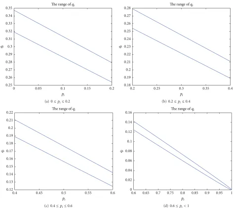
According to the character of Normal Distribution,

𝑃(|𝑞_𝑖−𝜇| < 3𝜎) ≈ 0.9974. So we can regard that_max𝑞_𝑖= 𝜇+3𝜎 and _min𝑞_𝑖 = 𝜇 − 3𝜎. Figure 2 illustrates the range of𝑞_𝑖 for different values of𝑝_𝑖when𝑛 = 104and𝑐 = 4.

4.2. The Distribution of Reconstructed Positive Survey. There are some differences between reconstructing positive survey from a given negative survey and traditional method for parameter estimating. The reason is that the given result of negative survey is only one sample for its original positive survey. In consequence, we use Bayes method to reconstruct the positive survey. The distribution of the reconstructed𝑝_𝑖 is given in Theorem 2.

Theorem 2. If a negative category is𝑁𝑆(𝑛, 𝑐, 𝑞_𝑖), the

probabil-ity densprobabil-ity function of corresponding𝑃𝑆(𝑛, 𝑐, 𝑝_𝑖)is

𝜋 (𝑝𝑖| 𝑞𝑖) = 𝑒

−𝑛[(𝑐−1)𝑞𝑖−(1−𝑝𝑖)]2/2(𝑐−2)(1−𝑝𝑖)_{/√1 − 𝑝}

𝑖 ∫₀1𝑒−𝑛[(𝑐−1)𝑞𝑖−(1−𝑝)]2/2(𝑐−2)(1−𝑝)/√1 − 𝑝_d𝑝. (8)

Proof. Define𝜋(𝑝_𝑖)to be the prior probability density func-tion of 𝑝_𝑖, and 𝑃(𝑞_𝑖 | 𝑝_𝑖) is the conditional probability density function for𝑞_𝑖. According to Bayes function form of probability density function, the probability density function of𝑝_𝑖with given𝑞_𝑖is the following formula:

𝜋 (𝑝𝑖| 𝑞𝑖) = 𝑃 (𝑞𝑖| 𝑝𝑖) 𝜋 (𝑝𝑖)

∫₀1𝑃 (𝑞_𝑖| 𝑝) 𝜋 (𝑝)d𝑝. (9)

Suppose that we have no knowledge of 𝑝_𝑖. Based on Bayesian assumption, the prior probability density function

𝜋(𝑝_𝑖)can be considered as uniform distribution𝑈(0, 1). On this occasion, the density function𝜋(𝑝_𝑖)can be calculated in the following Formula (10). In addition, 𝑃(𝑞_𝑖 | 𝑝_𝑖) can be calculated in Formula (7). Consider the following:

𝜋 (𝑝_𝑖) = 1, 0 < 𝑝_𝑖< 1,

𝜋 (𝑝_𝑖) = 0, otherwise. (10)

So the conditional probability density function of 𝑝_𝑖 with given𝑞_𝑖is

𝜋 (𝑝_𝑖| 𝑞_𝑖) = 𝑃 (𝑞𝑖| 𝑝𝑖)

∫₀1𝑃 (𝑞_𝑖| 𝑝_𝑖)d𝑝_𝑖. (11)

Combing Formula (7) and Formula (11), Formula (8) can be gotten and Theorem 2 is valid.

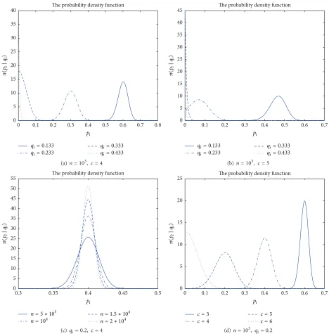
Figure 3 illustrates the function curve of 𝜋(𝑝_𝑖 | 𝑞_𝑖)for different values of𝑞_𝑖,𝑛, or𝑐. Figures 3(a) and 3(b) show that less𝑞_𝑖makes𝑝_𝑖centred around1 − (𝑐 − 1)𝑞_𝑖 more closely, Figure 3(c) shows that greater𝑛makes that, and Figure 3(d) shows that less𝑐makes that, too. In addition, Figures 3(a) and 3(b) also show that greater𝑞_𝑖may lead to1 − (𝑐 − 1)𝑞_𝑖 < 0, and the corresponding𝑝_𝑖is 0 with a great probability.

4.3. The Confidence Level. In this subsection, an approxi-mation method is used for calculating confidence level of reconstructed positive survey.

Theorem 3. If confidence interval length is𝛿, the confidence

level1 − 𝛼is

1 − 𝛼 = { { { { { { {

𝑃 (̂𝑝_𝑖−𝛿₂ ≤ 𝑝_𝑖≤ ̂𝑝_𝑖+𝛿₂) = ∫𝑝̂𝑖+𝛿/2 ̂ 𝑝𝑖−𝛿/2

𝜋 (𝑝_𝑖| 𝑞_𝑖)d𝑝_𝑖, 𝑞_𝑖< 1 − 𝛿/2

𝑐 − 1 , 𝑃 (0 ≤ 𝑝𝑖≤ 𝛿) = ∫

𝛿

0 𝜋 (𝑝𝑖| 𝑞𝑖)d𝑝𝑖, 𝑞𝑖≥ 1 − 𝛿/2

𝑐 − 1 ,

(12)

where𝑝̂_𝑖= 1 − (𝑐 − 1)𝑞_𝑖, and𝜋(𝑝_𝑖| 𝑞_𝑖)is in Formula (8).

Proof. According to Theorem 2, Theorem 3 is valid obviously.

Figure 4 illustrates the confidence level varying with𝑞_𝑖 with different values of𝑛and𝑐. From this figure, obviously the confidence level has the following two characters: (1) when𝑞_𝑖 < (1 − 𝛿/2)/(𝑐 − 1), the confidence level increases with𝑛(Figure 4(c)) and decreases with𝑞_𝑖(Figure 4(a)) or𝑐 (Figure 4(b));(2)when𝑞_𝑖≥ (1 − 𝛿/2)/(𝑐 − 1), the confidence level increases with 𝑞_𝑖 firstly (Figure 4(d)). Because in this case the𝑝_𝑖is 0 with a high probability, the confidence level decreases severely (Figure 4(d)). These values of𝑞_𝑖are nearly impossible because the prior probability to attain such a large

value of𝑞_𝑖 is very low, and𝑞_𝑖 may be the survey error (if

𝑞_𝑖> 𝜇 + 3𝜎as described in Section 4.1).

5. Simulation Experiments

In this section, some examples of negative survey (similar with that in [12]) are specially designed to verify this approx-imation method. In Tables 1 and 2, the confidence level is calculated independently by category when the confidence interval (abbreviated as CI) length is 0.1. As is indicated in Table 1, the confidence interval is (̂𝑝_𝑖 − 𝛿/2, ̂𝑝_𝑖 + 𝛿/2) as

(6)

The probability density function

qi= 0.133

qi= 0.233

qi= 0.333

qi= 0.433

0.1 0.2 0.3 0.4 0.5 0.6 0.7 0.8

0

pi

0 5 10 15 20 25 30 35 40

𝜋(

pi |qi

)

(a)𝑛 = 103, 𝑐 = 4

qi= 0.133

qi= 0.233

qi= 0.333

qi= 0.433

0.1 0.2 0.3 0.4 0.5 0.6 0.7

0

pi

0 5 10 15 20 25 30 35 40 45

𝜋(

pi |qi

)

(b) 𝑛 = 103, 𝑐 = 5

n = 5 ∗ 103

n = 104 n = 1.5 ∗ 10

4

n = 2 ∗ 104

0 5 10 15 20 25 30 35 40 45 50 55

0.35 0.4 0.45 0.5

0.3

pi

𝜋(

pi |qi

)

(c)𝑞_𝑖= 0.2, 𝑐 = 4

0 5 10 15 20 25

0.1 0.2 0.3 0.4 0.5 0.6 0.7

0

pi

c = 3

c = 4 c = 5c = 6

𝜋(

pi |qi

)

(d)𝑛 = 103, 𝑞_𝑖= 0.2

Figure 3: The function curve of𝜋(𝑝_𝑖| 𝑞_𝑖)with different values of𝑞_𝑖,𝑐, or𝑛.

prior probability to attain such a greater value of𝑞_𝑖is very low. In addition, when𝑝̂_𝑖is a negative value, the second method in [11] is needed to correct the reconstructed positive survey. Table 3 shows the confidence levels of seven groups of negative survey. The confidence level includes three values, which is the confidence level of each category, respectively. It is worth reminding that the confidence levels in the last three groups of negative survey are less when𝑛 = 1000. The reason that the probability to get such a large value of𝑞_𝑖is rather low if𝑛 = 1000. When𝑛 = 1000, the confidence levels of the last three groups of negative survey are low, and the survey results may be faulty.

6. Discussion

In this study, we propose an efficient approximation method for calculating the confidence level of negative survey, but there are some works for future study.

(7)

The confidence level

𝛿 = 0.01

𝛿 = 0.02 𝛿 = 0.03𝛿 = 0.04

0.3 0.4 0.5 0.6 0.7 0.8 0.9 1

1−

𝛼

0.05 0.1 0.15 0.2 0.25 0.3

0

qi

(a)𝑛 = 104, 𝑐 = 4

c = 3

c = 4 c = 5c = 6

0.2 0.3 0.4 0.5 0.6 0.7 0.8 0.9 1

1−

𝛼

0.02 0.04 0.06 0.08 0.1 0.12 0.14 0.16

0

qi

(b) 𝑛 = 104, 𝛿 = 0.01

n = 2 ∗ 103

n = 4 ∗ 103 n = 6 ∗ 10

3

n = 8 ∗ 103

0.05 0.1 0.15 0.2 0.25 0.3

0

qi

0.1 0.2 0.3 0.4 0.5 0.6 0.7 0.8 0.9 1

1−

𝛼

(c) 𝑐 = 4, 𝛿 = 0.01

n = 2 ∗ 103

n = 4 ∗ 103 n = 6 ∗ 10

3

n = 8 ∗ 103

0.36 0.38 0.4 0.42 0.44 0.46 0.48 0.5

0.34

qi

0 0.1 0.2 0.3 0.4 0.5 0.6 0.7 0.8 0.9 1

1−

𝛼

(d)𝑐 = 4, 𝛿 = 0.01

Figure 4: The confidence level of estimated𝑝_𝑖varying with𝑞_𝑖,𝑐, or𝑛.

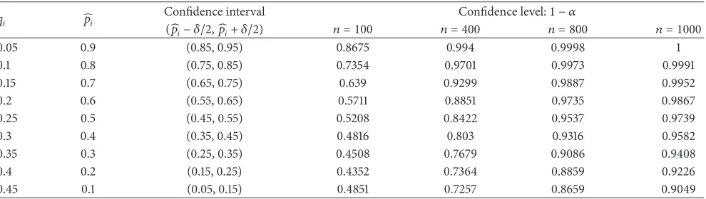
Table 1: The confidence level as𝑞_𝑖< (1 − 𝛿/2)/(𝑐 − 1)(𝛿 = 0.1,𝑐 = 3).

𝑞𝑖 𝑝̂𝑖 Confidence interval_(̂_𝑝 Confidence level:1 − 𝛼

𝑖− 𝛿/2,𝑝̂𝑖+ 𝛿/2) 𝑛 = 100 𝑛 = 400 𝑛 = 800 𝑛 = 1000

0.05 0.9 (0.85, 0.95) 0.8675 0.994 0.9998 1

0.1 0.8 (0.75, 0.85) 0.7354 0.9701 0.9973 0.9991

0.15 0.7 (0.65, 0.75) 0.639 0.9299 0.9887 0.9952

0.2 0.6 (0.55, 0.65) 0.5711 0.8851 0.9735 0.9867

0.25 0.5 (0.45, 0.55) 0.5208 0.8422 0.9537 0.9739

0.3 0.4 (0.35, 0.45) 0.4816 0.803 0.9316 0.9582

0.35 0.3 (0.25, 0.35) 0.4508 0.7679 0.9086 0.9408

0.4 0.2 (0.15, 0.25) 0.4352 0.7364 0.8859 0.9226

(8)

Table 2: The confidence level as𝑞_𝑖≥ (1 − 𝛿/2)/(𝑐 − 1)(𝛿 = 0.1,𝑐 = 3).

𝑞_𝑖 𝑝̂_𝑖 Confidence interval(0,𝛿) Confidence level:1 − 𝛼

𝑛 = 100 𝑛 = 400 𝑛 = 800 𝑛 = 1000

0.5 0 (0, 0.1) 0.7198 0.9665 0.9973 0.9992

0.55 −0.1 (0, 0.1) 0.8949 0.9995 1 1

0.6 −0.2 (0, 0.1) 0.9674 0.9933 0.2612 0.2115

0.7 −0.4 (0, 0.1) 0.9881 0.2433 0.1336 0.1171

0.8 −0.6 (0, 0.1) 0.5796 0.1568 0.1064 0.1022

Table 3: The confidence level as𝛿 = 0.1and𝑐 = 3.

(𝑞₁,𝑞₂,𝑞₃) (̂𝑝₁,𝑝̂₂,𝑝̂₃) Confidence level:1 − 𝛼

𝑛 = 100 𝑛 = 1000

(0.35, 0.35, 0.3) (0.3, 0.3, 0.4) (0.451, 0.451, 0.482) (0.941, 0.941, 0.958)

(0.4, 0.3, 0.3) (0.2, 0.4, 0.4) (0.435, 0.482, 0.482) (0.923, 0.958, 0.958)

(0.45, 0.3, 0.25) (0.1, 0.4, 0.5) (0.485, 0.482, 0.521) (0.905, 0.958, 0.974)

(0.5, 0.3, 0.2) (0, 0.4, 0.6) (0.720, 0.482, 0.571) (0.999, 0.958, 0.987)

(0.6, 0.3, 0.1) (−0.2, 0.4, 0.8) (0.967, 0.482, 0.735) (0.212, 0.958, 0.999)

(0.7, 0.2, 0.1) (−0.4, 0.6, 0.8) (0.988, 0.571, 0.735) (0.117, 0.987, 0.999)

(0.8, 0.15, 0.05) (−0.6, 0.7, 0.9) (0.580, 0.639, 0.868) (0.102, 0.995, 1)

than Normal Distribution. In addition, Normal Distribution, which is a symmetric distribution, is used to approximate the original distribution, but the original distribution is not perfectly symmetrical.

Secondly, this method in this study analyses each category independently. The correlation of different categories should be taken into account in future work. For example, the confidence level may be high when𝑞_𝑖 ≥ 1/(𝑐 − 1), because the corresponding𝑝_𝑖has a high probability to be 0. But in this case, the sum of all the estimated𝑝_𝑖is greater than 1, and the results are needed for further revision.

Thirdly, the confidence interval is set to be(𝜇 − 𝛿/2, 𝜇 +

𝛿/2)when𝑞_𝑖 < 1/(𝑐 − 1). But strictly,𝜋(𝑝_𝑖 | 𝑞_𝑖) is not a completely symmetrical function. So the confidence interval may not be the smallest one.

Finally, the confidence level calculated in this study is by category independently. How to compare the two close confidence levels (such as the first two examples in Table 3) still needs to be studied further.

7. Conclusions

This study proposes an efficient approximation method for calculating the confidence level of negative survey. Normal Distribution is used to approximate to the distribution of𝑞_𝑖at first; then Bayes method is used for approximately calculating the confidence level. Depending on the proposed efficient approximation method, the confidence level of negative survey can be approximately calculated efficiently.

Conflict of Interests

The authors declare that there is no conflict of interests regarding the publication of this paper.

Acknowledgments

The project was supported by the National Natural Science Foundation of China under Grants 61502440, 61502439, and 61272469 and the Fundamental Research Funds for the Central Universities, China University of Geosciences (Wuhan), under Grant CUGL 140840.

References

[1] S. A. Hofmeyr and S. Forrest, “Architecture for an artificial immune system,”Evolutionary Computation, vol. 8, no. 4, pp. 443–473, 2000.

[2] S. Forrest, A. S. Perelson, L. Allen, and R. Cherukuri, “Self-nonself discrimination in a computer,” inProceedings of the IEEE Symposium on Research in Security and Privacy, pp. 202– 212, May 1994.

[3] J. Kim and P. J. Bentley, “Towards an artificial immune system for network intrusion detection: an investigation of clonal selection with a negative selection operator,” inProceedings of the Congress on Evolutionary Computation (CEC ’01), vol. 2, pp. 1244–1252, May 2001.

[4] G. Du, T. Huang, B. Zhao, and L. Song, “Dynamic self-defined immunity model base on data mining for network intrusion detection,” inProceedings of the 4th International Coference on Machine Learning and Cybernetics, vol. 6, pp. 3866–3870, 2005. [5] Z. Ji and D. Dasgupta, “V-detector: an efficient negative selec-tion algorithm with ‘probably adequate’ detector coverage,” Information Sciences, vol. 179, no. 10, pp. 1390–1406, 2009. [6] F. Esponda, “Negative surveys,” http://arxiv.org/abs/math/

0608176.

(9)

[8] F. Esponda and V. M. Guerrero, “Surveys with negative ques-tions for sensitive items,”Statistics and Probability Letters, vol. 79, no. 24, pp. 2456–2461, 2009.

[9] J. L. Horey, S. Forrest, and M. Groat, “Reconstructing spatial distributions from anonymized locations,” inProceedings of the 28th International Conference on Data Engineering Workshops, pp. 243–250, ACM, 2012.

[10] H. Xie, L. Kulik, and E. Tanin, “Privacy-aware collection of aggregate spatial data,”Data & Knowledge Engineering, vol. 70, no. 6, pp. 575–595, 2011.

[11] Y. Bao, W. Luo, and X. Zhang, “Estimating positive surveys from negative surveys,”Statistics and Probability Letters, vol. 83, no. 2, pp. 551–558, 2013.

(10)

Submit your manuscripts at

http://www.hindawi.com

Hindawi Publishing Corporation

http://www.hindawi.com Volume 2014

Mathematics

Journal of

http://www.hindawi.com Volume 2014 Mathematical Problems in Engineering

Hindawi Publishing Corporation http://www.hindawi.com

Differential Equations International Journal of

Volume 2014

http://www.hindawi.com Volume 2014 Hindawi Publishing Corporationhttp://www.hindawi.com Volume 2014

http://www.hindawi.com Volume 2014 Mathematical PhysicsAdvances in

Complex Analysis

Journal of

Optimization

Journal of

Combinatorics

International Journal of

Journal of

Function Spaces

Abstract and Applied Analysis

International Journal of Mathematics and Mathematical Sciences

Hindawi Publishing Corporation http://www.hindawi.com Volume 2014

The Scientific

World Journal

Discrete Dynamics in Nature and Society Hindawi Publishing Corporation

http://www.hindawi.com Volume 2014 Hindawi Publishing Corporation

Discrete Mathematics

Journal of

http://www.hindawi.com Volume 2014 Hindawi Publishing Corporationhttp://www.hindawi.com Volume 2014