A CNN-BASED FUSION METHOD FOR FEATURE
2EXTRACTION FROM SENTINEL DATA
3Giuseppe Scarpa1*, Massimiliano Gargiulo1, Antonio Mazza1and Raffaele Gaetano2 4
1 DIETI, University Federico II, Via Claudio 21, 80125 Naples, Italy 5
2 UMR-TETIS Laboratory, CIRAD, 34000 Montpellier, France 6
* Correspondence: [email protected]; Tel.: +39 081 768 3768 7
Abstract: Sensitivity to weather conditions, and specially to clouds, is a severe limiting factor
8
to the use of optical remote sensing for Earth monitoring applications. A possible alternative,
9
is to resort to weather-insensitive synthetic aperture radar (SAR) images. However, in many
10
real-world applications, critical decisions are made based on some informative spectral features,
11
such as water, vegetation or soil indices, which cannot be extracted from SAR images. In the
12
absence of optical sources, these data must be estimated. The current practice is to perform linear
13
interpolation between data available at temporally close time instants. In this work, we propose
14
to estimate missing spectral features through data fusion and deep-learning. Several sources of
15
information are taken into account - optical sequences, SAR sequences, DEM - so as to exploit both
16
temporal and cross-sensor dependencies. Based on these data, and a tiny cloud-free fraction of
17
the target image, a compact convolutional neural network (CNN) is trained to perform the desired
18
estimation. To validate the proposed approach, we focus on the estimation of the normalized
19
difference vegetation index (NDVI), using coupled Sentinel-1 and Sentinel-2 time-series acquired
20
over an agricultural region of Burkina Faso from May to November 2016. Several fusion schemes
21
are considered, causal and non-causal, single-sensor or joint-sensor, corresponding to different
22
operating conditions. Experimental results are very promising, showing a significant gain over
23
baselines methods according to all performance indicators.
24
Keywords: Coregistration; pansharpening; multi-sensor fusion; multitemporal images; deep
25
learning; normalized difference vegetation index (NDVI).
26
PACS:J0101
27
1. Introduction 28
The recent launch of coupled optical/SAR (synthetic aperture radar) Sentinel satellites, in the
29
context of the Copernicus program, opens unprecedented opportunities for end users, both industrial
30
and institutional, and poses new challenges to the remote sensing research community. The policy of
31
free distribution of data allows large scale access to a very rich source of information. Besides this,
32
the technical features of the Sentinel constellationmakes it a precious tool for a wide array of remote
33
sensing applications. With revisit time ranging from two days to about a week, depending on the
34
geographic location, spatial resolution from 5 to 60 meters, and wide coverage of the spectrum, from
35
visible to short-wave infrared (∼ 440−2200 nm), Sentinel data may impact decisively on a number
36
of Earth monitoring applications, such as climate change monitoring, map updating, agriculture and
37
forestry planning, flood monitoring, ice monitoring, and so forth.
38
Especially precious is the diversity of information guaranteed by the coupled SAR and optical
39
sensors, a key element for boosting the monitoring capability of the constellation. In fact, the
40
information conveyed by the Sentinel-2 (S2) multi-resolution optical sensor depends on the spectral
41
reflectivity of the target illuminated by sunlight, while the backscattered signal acquired by the
42
Sentinel-1 (S1) SAR sensor depends on both target’s characteristics and the illuminating signal.
43
The joint processing of optical and radar temporal sequences offers the opportunity to extract the
44
information of interest with an accuracy that could not be achieved based on only one these sources.
45
Of course, with this potential, comes the scientific challenge of how to exploit these complementary
46
piece information in the most effective way.
47
In this work, we focus on the estimation of the Normalized Difference Vegetation Index (NDVI)
48
in critical weather conditions, fusing the information provided by temporal sequences of S1 and S2
49
images. In fact, the typical processing pipelines of many land monitoring applications rely, among
50
other features, on the NDVI for a single date or a whole temporal series. Unfortunately, the NDVI,
51
as well as other spectral features, is unavailable under cloudy weather conditions. The commonly
52
adopted solution consists in interpolating between temporally adjacent images where the target
53
feature is present. However, given the availability of weather-insensitive SAR data of the scene,
54
it make sense to pursue fusion-based solutions, exploiting SAR images that may be temporally very
55
close to the target date. By so doing, we assume that SAR data, despite their very different nature, can
56
provide precious information on NDVI. Even if this holds true, however, it is by no means obvious
57
how to exploit such dependency. To address this problem we resort to deep learning, designing
58
a simple three-layer convolutional neural network (CNN) for this task, and training it to account
59
for both temporal and cross-sensor dependencies. Note that the same approach, with minimal
60
adaptations, can be extended to estimate many other spectral indices, commonly used for water,
61
soil, and so on. Therefore, besides solving the specific problem, we demonstrate the potential of deep
62
learning for data fusion in remote sensing.
63
According to the taxonomy given in [1] data fusion methods,i.e.,processing dealing with data and 64
information from multiple sources to achieve improved information for decision making, can be grouped in
65
three main categories:
66
– pixel-level: the pixel values of the sources to be fused are jointly processed [2–5];
67
– feature-level: features like lines, regions, keypoints, maps, and so on, are first extracted
68
independently from each source image and subsequently combined to produce higer-level
69
cross-source features which may represent the desired output or be further processed [6–12];
70
and
71
– decision-level: the high-level information extracted independently from each source is combined
72
to provide the final outcome, for example resorting to fuzzy logic [13,14], decision trees [15],
73
Bayesian inference [16], Dempster-Shafer theory [17], and so forth.
74
In the context of remote sensing, with reference to the sources to be fused, fusion methods can
75
be roughly gathered for the most part in the following categories:
76
– multi-resolution: concerns a single sensor with multiple resolution bands. One of the most
77
frequent application is pansharpening [2,18,19], although many other tasks can be solved under
78
a multi-resolution paradigm, such as segmentation [20] or feature extraction [21], to mention a
79
few.
80
– multi-temporal: is one of the most investigated forms of fusion in remote sensing due to the
81
rich information content hidden in the temporal dimension. In particular it can be applied to
82
strictly time-related tasks, like prediction [9], change detection [22,23], co-registration [24], and
83
general-purpose tasks, like segmentation [3], despeckling [25], feature extraction [26–28], which
84
do not necessarily need a joint processing of the temporal sequence but can benefit from it.
85
– multi-sensor: is gaining an ever growing importance due both to the recent deployment of many
86
new satellites, and to the increasing tendency of the community to share data. It represents also
87
the most challenging case because of the several sources of mismatch (temporal, geometrical,
88
spectral, radiometrical) among involved data. Like for other categories, a number of typical
89
remote sensing problems can fit this paradigm, such as classification [6,12,29–31], coregistration
90
[11], change detection [32], feature estimation [33–36].
91
– mixed: the above cases may also occur jointly, generating mixed situations. For example
92
hyperspectral and multiresolution images can be fused to produce a spatial-spectral
93
full-resolution datacube [5,37]. Likewise, low-resolution temporally dense series can be fused
with high-resolution but temporally sparse ones to simulate a temporal-spatial full-resolution
95
sequence [38]. The monitoring of forests [16], soil moisture [39], environmental hazards [8], and
96
other processes, can be also carried out effectively by fusing SAR and optical time series. Finally,
97
works that mix all three aspects, resolution, time, and sensor, can also be found in the literature
98
[7,17,40].
99
Turning to multi-sensor SAR-optical fusion for the purpose of vegetation monitoring, a number
100
of contributions can be found in the literature [7,12,16,34,41]. In [7] ALOS POLSAR and Landsat
101
time-series were combined at feature level for forest mapping and monitoring. The same problem
102
was addressed in [16] through a decision-level approach. In [41] the fusion of single-date S1 and
103
simulated S2 was presented for the purpose of classification. In [34], instead, RADARSAT-2 and
104
Landsat-7/8 images were fused, by means of an artificial neural network, to estimate soil moisture
105
and leaf area index. The NDVI index obtained from the Landsat source was combined with different
106
SAR polarization subsets for feeding ad hoc artificial networks. A similar feature-level approach,
107
based on Sentinel data, was followed in [12] for the purpose of land cover mapping. To this end,
108
the texture maps extracted from the SAR image were combined with several indices drawn from the
109
optical bands.
110
Although some fusion techniques have been proposed for spatio-temporal NDVI
111
super-resolution [38] or prediction [9], they use exclusively optical data. None of these papers
112
attempts to directly estimate a pure multispectral feature, NDVI or the likes, from SAR data. In most
113
cases the fusion, occurring already at feature level, is intended to provide high-level information,
114
like the classification or detection of some physical item. Conversely, we can register some notable
115
example of indices directly related to physical items of interest, like soil moisture or the area leaf
116
index, which have been estimated by fusing SAR and optical data [33,34].
117
In this work, we propose several CNN-based algorithms to estimate the NDVI through the
118
fusion of optical and SAR Sentinel data. With reference to a specific case study, we acquired temporal
119
sequences of S1 SAR data and S2 optical data, covering the same time lapse, with the latter partially
120
covered by clouds. Both temporal and cross-sensor (S1-S2) dependencies are used to obtain the
121
most effective estimation protocol. From the experimental analysis, very interesting results emerge.
122
On one hand, when only optical data are used, CNN-based methods outperform consistently the
123
conventional temporal interpolators. On the other hand, when also SAR data are considered, a further
124
significant improvement of performance is observed, despite the very different nature of the involved
125
signals. It is worth underlining that no peculiar property of NDVI was exploited, and therefore these
126
results have a wider significance, suggesting that other image features can be better estimated by
127
cross-sensor CNN-based fusion.
128
The rest of the paper is organized as follows. In Section 2, we present the dataset and describe
129
the problem under investigation. In Section 3, the basics of the CNN methodology are recalled. Then,
130
the specific prediction architectures are detailed in Section 4. Finally, in Section 5, we present and
131
discuss the experimental results. Section 6 draws conclusions.
132
2. Dataset and Problem Statement 133
The objective of this work is to propose and test a set of solutions to estimate a target optical
134
feature at a given date from images acquired at adjacent dates, or even from the temporally closest
135
SAR image. Such different solutions reflect also the different operating conditions found in practice.
136
The main application is the reconstruction of a feature of interest in a target image which is available
137
but partially or totally cloudy. However, one may also consider the case in which the feature is built
138
and used on a date for which no image is actually available.
139
ma
y-05may-15 jun-04 aug-03 sep-02 oct-12 nov-01
100
time line % available data (cloud free)
S1 - selected
S1 - discarded
S2 - selected
S2 - discarded
Figure 1. Available S1 (black) and S2 (green) images over the period of interest. The bar height indicates the fraction of usable data. Solid bars mark selected images, boldface date mark test images.
images, the NDVI is obtained at a resolution of 10 meters by combining pixel-by-pixel two bands, near infrared (NIR, 8th band), and red (Red, 4th band), as:
NDVI, NIR−Red
NIR+Red ∈ [−1, 1] (1)
The area under study is located in the province of Tuy, Burkina Faso, around the commune of
140
Koumbia. This area is particularly representative of West African semiarid agricultural landscapes,
141
for which the Sentinel missions offer new opportunities in monitoring vegetation, notably in the
142
context of climate change adaptation and food security. The use of SAR data in conjunction with
143
optical images is particularly appropriate in these areas, since most of the vegetation dynamics take
144
place during the rainy season, especially over the cropland, as smallholder rainfed agriculture is
145
dominant. This strongly reduces the availability of usable optical images in the critical phase of
146
vegetation growth, due to the significant cloud coverage [42] from which SAR data are only loosely
147
affected. The 5253x4797 pixels scene is monitored between May 5th and November 1st 2016, over a
148
period that corresponds to a regular cultural season in the area.
149
Fig.1indicates the available S1 and S2 acquisitions in this period. In the case of S2 images, the bar
150
height indicates the percentage of data which are not cloudy. It is clear that some dates provide little
151
or no information. Note that, during the rainy season, the lack of sufficient cloud-free optical data
152
may represent a major issue, preventing the extraction of spatio-temporal optical-based features, like
153
time-series of vegetation, water or soil indices, and so on. S1 images, instead, are always completely
154
available, as SAR data are insensitive to meteorological conditions.
155
For the purpose of training, validation and testing of the proposed methods, we kept only S2
156
images which were cloud-free, or such that the spatial distribution of clouds did not prevent the
157
selection of sufficiently large test and training areas. For the selected S2 images (solid bars in Fig.1)
158
the corresponding dates are indicated on thex-axis. Our dataset was then completed by including
159
also the S1 images (solid bars) which are temporally closest to the selected S2 counterparts. The
160
general idea of the proposal is to use the closest cloud-free S2 and S1 images to estimate the desired
161
feature on the target date of interest. Therefore, among the seven selected dates, only the five inner
162
ones are used as targets. Observe, also, that the resulting temporal sampling is rather variable, with
163
intervals ranging from ten days to a couple of months, allowing us to test our methods in different
164
conditions.
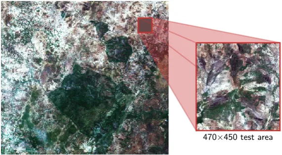
470×450 test area
Figure 2.RGB false-color representation of the 5253×4797 S2-Koumbia dataset (May 15th, 2016), with a zoom on the area selected for testing.
To allow also temporal analyses, we chose a test area, of size 470×450, which is cloud-free in all
166
the selected dates, and hence with available reference ground-truth for any possible optical feature.
167
Fig.2 shows a false-color representation of a complete image of the Koumbia dataset (May 15th,
168
2016), together with a zoom of the selected test area. Even after discarding the test area, quite a large
169
usable area remains, from which a sufficiently large number of small (33×33) cloud-free patches are
170
randomly extracted for training and validation.
171
In addition to the Sentinel data, we assume the availability of two additional features, the cloud
172
masks for each S2 image, and a Digital Elevation Model (DEM). Cloud masks are obviously necessary
173
to establish when the prediction is needed and which adjacent dates should be involved. The DEM is
174
a complementary feature that integrates the information carried by SAR data, and may be useful to
175
improve estimation.
176
For this work, we used Sentinel-1 data in the Ground Range Detected (GRD) format as
177
provided by ESA. All images have been calibrated (VH/VV intensities to sigma nought) and
178
terrain corrected using ancillary data, and co-registered to provide a 10 m resolution, spatially
179
coherent time series, using the official ESA Sentinel Application Platform (SNAP) software [43]. No
180
optical/SAR co-registration has been performed, assuming that the co-location precision provided
181
by the independent orthorectification of each product is sufficient for the application. Sentinel-2 data
182
are provided by the French Pole Thématique Surfaces Continentales (THEIA) [44] and preprocessed
183
using the Multi-sensor Atmospheric Correction and Cloud Screening (MACCS) level 2A processor
184
[45] developed at the French National Space Agency (CNES) to provide surface reflectance products
185
as well as precise cloud masks. Finally, the DEM was gathered from the Shuttle Radar Topographic
186
Mission (SRTM) 1 Arc-Second Global, with 30 m resolution resampled at 10 m to match the spatial
187
resolution of Sentinel data.
188
3. Convolutional neural networks 189
Before moving to the specific solutions for NDVI estimation, in this Section we provide some
190
basic notions and terminology about CNNs.
191
In the last few years, convolutional neural networks have been successfully applied to many
192
classical image processing problems, such as denoising [46], super-resolution [47], pansharpening
193
[4,19], segmentation [48], detection [49], classification [50,51]. The main strengths of CNNs are (i) an
194
extreme versatility that allows them to approximate any sort of linear or non linear transformation,
195
including scaling or hard thresholding; (ii) no need to design handcrafted filters, replaced by machine
196
learning; (iii) high-speed processing, thanks to parallel computing. On the downside, for correct
197
training, CNNs require the availability of a large amount of data with ground-truth (examples). In our
specific case, data are not a problem, given the unlimited quantity of cloud-free Sentinel-2 time-series
199
that can be downloaded from the web repositories. However, using large datasets has a cost in terms
200
of complexity, and may lead to unreasonably long training times. Usually, a CNN is a chain1 of
201
different layers, like convolution, nonlinearities, pooling, deconvolution. For image processing tasks
202
in which the desired output is an image at the same resolution of the input, as in this work, only
203
convolutional layers interleaved with nonlinear activations are typically employed.
204
The generic l-th convolutional layer, with N-band input x(l), yields an M-band output z(l)
computed as
z(l)=w(l)∗x(l)+b(l),
whosem-th component can be written in terms ordinary 2D convolutions
z(l)(m,·,·) =
N
∑
n=1
w(l)(m,n,·,·)∗x(l)(n,·,·) +b(l)(m).
The tensorwis a set ofMconvolutionalN×(K×K)kernels, with aK×Kspatial support (receptive field), whilebis aM-vector bias. These parameters, compactly,Φl ,
w(l),b(l), are learnt during the training phase. If the convolution is followed by a pointwise activation functiongl(·), then, the
overall layer output is given by
y(l)=gl(z(l)) =gl(w(l)∗x(l)+b(l)), fl(x(l),Φl). (2)
Due to the good convergence properties it ensures [50], the Rectified Linear Unit (ReLU), defined as
205
g(·),max(0, ·), is a typical activation function of choice for input or hidden layers.
206
Assuming a simpleL-layer cascade architecture, the overall processing will be
f(x,Φ) = fL(fL−1(. . .f1(x,Φ1), . . . ,ΦL−1),ΦL) (3)
whereΦ,(Φ1, . . . ,ΦL)is the whole set of parameters to learn. In this chain, each layerlprovides a
207
set of so-calledfeature maps,y(l), which activate on local cues in the early stages (smalll), to become
208
more and more representative of abstract and global phenomena in subsequent ones (largel). In this
209
work, all proposed solutions are based on a simple three-layer architecture, and differ only in the
210
input layer, as different combinations of input bands are considered.
211
3.1. Learning 212
In order to learn the network parameters, a sufficiently large training set, sayT, of input-output examplestis needed:
T,{t1, . . . ,tQ}, t,(x,yref)
In our specific case,xwill be a sample of the combination of images from which we want to estimate
213
the target NDVI map, withyrefthe desired output. Of course, all involved optical images must be
214
cloud-free over the selected patches.
215
Formally, the objective of the training phase is to find
Φ=arg min
Φ J(T,Φ),arg minΦ
1
Qt
∑
∈TL(t,Φ)whereL(t,Φ)is a suitable loss function. Several losses can be found in the literature, likeLnnorms,
cross-entropy, negative log-likelihood. The choice depends on the domain of the output, and affects
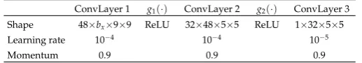
Table 1.Hyper-parameters of the CNN architecture. Shape = # features×# channels×2D support.
ConvLayer 1 g1(·) ConvLayer 2 g2(·) ConvLayer 3 Shape 48×bx×9×9 ReLU 32×48×5×5 ReLU 1×32×5×5
Learning rate 10−4 10−4 10−5
Momentum 0.9 0.9 0.9
the convergence properties of the networks [52]. Among the different solutions experimented, which will be later discussed, we have chosen theL1-norm
L(t,Φ)∝||f(x,Φ)−yref||1 (4)
which proved effective in other generative problems in remote sensing [19]. As for minimization, the
216
most widespread procedure, adopted also in this work, is the stochastic gradient descent (SGD) with
217
momentum [53]. The training set is partitioned in batches of samples, T = {B1, . . . ,BP}. At each
218
iteration, a new batch is used to estimate the gradient and update parameters as
219
ν(n+1)←µν(n)+α∇ΦJ
Bjn,Φ
(n)
Φ(n+1)←Φ(n)− ν(n+1)
A whole scan of the training set is called anepoch, and training a deep network may require from
220
dozens of epochs, for simpler problems like handwritten character recognition [54], to thousands
221
of epochs for complex classification tasks [50]. Accuracy and speed of training depend on both the
222
initialization ofΦand the setting of hyperparameters like learning rateαand momentumµ, withα 223
being to most critical, impacting heavily on stability and convergence time.
224
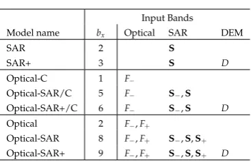
4. Proposed prediction architectures 225
In the following developments, with reference to a given target S2 image acquired at timet, we
226
will consider the items defined below:
227
• t−,t+: times of previous and next useful S2 images; 228
• tˆ, ˆt−, ˆt+: times of closest S1 image (always|t−tˆ| ≤5) and of previous and next S1 images;
229
• F: unknown feature (NDVI in this work) at timet;
230
• F−andF+: featureFat timest−andt+, respectively; 231
• S,(SVV,SV H): double polarized VV-VH SAR image at time ˆt;
232
• S−andS+: SAR images at times ˆt−and ˆt+, respectively; 233
• D: DEM.
234
The several models considered here differ in the composition of the input stackx, while the
235
output is always the NDVI at the target date, that is,y = F. Apart from the input layer, the CNN
236
architecture is always the same, depicted in Fig.3, with hyper-parameters summarized in Tab.1. This
237
relatively shallow CNN is characterized by a rather small number of weights (as CNNs go), and hence
238
can be trained with a small amount of data. On the other hand, this very same architecture has proven
239
to achieve state-of-the-art performance in closely related applications, such as super-resolution [47]
240
and data fusion [4,19].
241
The numberbxof input bands depends on the specific solution and will be made explicit below.
242
In order to provide output values falling in the compact interval [-1,1], as required by the NDVI
243
semantics (Eq.1), one can include a suitable nonlinear activation, like tanh(·), to complete the output
244
layer. In such a case, it is customary to resort to a cross-entropy loss for training. As an alternative, one
245
may remove the nonlinear output mapping altogether, and simply take the result of the convolution,
246
which can be optimized using, for example, a Ln-norm. Obviously, in this case, a hard clipping of
247
the output is still needed, but this additional transformation does not participate in the error back
S− F− S S+F+ DEM
input stack
| may-15 | jun-04 | aug-03 |
Sentinel-1 Sentinel-2
y(1)=f1(x,Φ 1)
y(2)=f2 y(1),Φ 2
y=f3 y(2),Φ 3
48 32
hidden layer
hidden layer
output layer
F
Figure 3. Proposed CNN architecture. The depicted input corresponds to the Optical-SAR+ case. Other cases use a reduced set of inputs.
Table 2.Proposed models.
Input Bands
Model name bx Optical SAR DEM
SAR 2 S
SAR+ 3 S D
Optical-C 1 F−
Optical-SAR/C 5 F− S−,S
Optical-SAR+/C 6 F− S−,S D
Optical 2 F−,F+
Optical-SAR 8 F−,F+ S−,S,S+
Optical-SAR+ 9 F−,F+ S−,S,S+ D
propagation, hence should be considered external to the network. Through preliminary experiments,
249
we have found this latter solution more effective than the former, for our task, and therefore we train
250
the CNN considering a linear activation in the last layer,g3(z(3)) = z(3). Experiments also showed 251
theL1-norm (Eq.4) to be more effective than theL2-norm for training, and hence we opted for the 252
former in our tests.
253
We now describe briefly the different solutions considered here, which depend on the available
254
input data and the required response time.
255
Concerning data, we will consider estimation based on optical-only, SAR-only, and optical+SAR
256
data. When using SAR images, we will also test the inclusion of the DEM, which may convey relevant
257
information on them. Instead, the DEM is useless, and hence neglected, when only optical data are
258
used. All these cases are of interest, for the following reasons.
259
– The optical-only case allows for a direct comparison, with the same input data, between
260
the proposed CNN-based solution and the current baseline, which relies on temporal linear
261
interpolation. Therefore, it will provide us with a measure the net performance gain guaranteed
262
by deep learning over conventional processing.
263
– Although SAR and optical data provide complementary information, the occurrence of a given
264
physical item, like water or vegetation, can be detected by means of both scattering properties
265
and spectral signatures. The analysis of the SAR-only case will allow us to understand if
266
significant dependencies exist between the NDVI and SAR images, and if a reasonable quality
267
can be achieved even when only this source is used for estimation. To this aim we do not count
268
on the temporal dependencies in this case trying to estimate a S2 feature from the closest S1
269
image only.
270
– Theoptical-SARfusion, of course, is the case of highest interest for us. Given the most complete
271
set of relevant input, and an adequate training set, the proposed CNN will synthesize expressive
272
features, and is expected to provide a high-quality NDVI estimate.
Turning to response time, except for the SAR-only case, we will distinguish between causal
274
estimation, in which only data already available at timet(or shortly later) can be used, and non-causal
275
estimation, when the whole time series is supposed to be available.
276
– Causal estimationis of interest whenever the data must be used right away for the application
277
of interest. This is the case, for example, of early warning systems for food security. We will
278
include here also the case in which ˆt>t, namely the closest SAR image becomes available after
279
timet, since the maximum delay is always very limited.
280
– On the other hand, in the absence of temporal constraints, all relevant data should be taken into
281
account to obtain the best possible quality, resorting therefore tonon-causal estimation.
282
Table.2summarizes all these different solutions.
283
4.1. Training 284
In order to carry out an effective training of the networks, a large cloud-free dataset is necessary,
285
with geophysical properties as close as possible to those of the target data. This is readily guaranteed
286
whenever all images involved in the process, for example F−,F and F+, share a relatively large 287
cloud-free area. Patches will be extracted from this area to train the network which, afterwards,
288
will be used to estimateFalso on the clouded area, obtaining a complete coverage at the target date.
289
For our relatively small network, a training+validation set of 18000 patches is sufficient for
290
accurate training. With our patch extraction process, this number requires an overall cloud-free area
291
of about 1000×1000 pixels, namely, about 4% of our 5253×4797 target scene (Fig.2). If the unclouded
292
regions are more scattered, this percentage may somewhat grow, but remains always quite limited.
293
Therefore, a perfectly fit training set will be available most of the times (always, in our experiments).
294
However, even if this is not the case, for example because the scene is almost completely covered
295
by clouds at the target date, one can build a good training set by using data collected on other
296
regions with geophysical features similar to those of the target scene (for example tropical-tropical).
297
Subsequently, even a very small unclouded region of the target scene can be used to fine-tune the
298
network parameters.
299
In practice, for each date, a dataset composed of 15200 33×33 examples for training, plus 3800
300
more for validation, was created by sampling the target scene with a 8-pixel stride in both spatial
301
directions, always skipping test area and cloudy regions. Then, the whole collection was shuffled to
302
avoid biases when creating the 128-examples mini-batches used in the SGD algorithm.
303
5. Experimental results 304
The performance of the proposed CNN-based estimators is assessed in terms of correlation index
305
(ρ), peak signal-to-noise ratio (PSNR), and structural similarity measure (SSIM). 306
We consider two reference methods, a deterministic linear interpolator (temporal gap-filling)
307
which can be regarded as the baseline, and a simple affine regressor. Temporal gap filling was
308
proposed in [42] in the context of the development of a national-scale crop mapping processor based
309
on Sentinel-2 time series, and implemented as a remote module of the Orfeo Toolbox [55]. This is a
310
practical solution used by analysts [42] to monitor vegetation processes through NDVI time-series.
311
Besides being simple, it is also more generally applicable and robust than higher-order models which
312
require a larger number of points to interpolate and may overfit the data. Since temporal gap filling
313
is non-causal, we add a further causal interpolator for completeness, a simple zero-order hold. Of
314
course, deterministic interpolation does not take into account the correlation between available and
315
target data, which can help performing a better estimate and can be easily computed based on a tiny
316
cloud-free fraction of the target image. Therefore, for a fairer comparison, we consider as a further
317
reference the affine regressors, both causal and non-causal, computed based on such correlations.
318
If suitable, post-processing may be included for spatial regularization, both for the reference and
319
proposed methods. This option is not pursued here.
Table 3.Correlation index,ρ∈[−1, 1].
may-15 jun-04 aug-03 sep-02 oct-12 average
gaps (before/after) 10/20 20/60 60/30 30/40 40/20
Cross-sensor SAR 0.8243 0.8161 0.5407 0.4219 0.4561 0.6118
SAR+ 0.8254 0.7423 0.3969 0.4963 0.6428 0.6207
Causal
Interpolator/C 0.9760 0.8925 0.6566 0.6704 0.6098 0.7611
Regressor/C 0.9760 0.8925 0.6566 0.6704 0.6098 0.7611
Optical/C 0.9811 0.9407 0.7245 0.7280 0.7302 0.8209
Optical-SAR/C 0.9797 0.9432 0.7716 0.7880 0.7546 0.8474
Optical-SAR+/C 0.9818 0.9424 0.7738 0.7855 0.7792 0.8525
Non-causal
Interpolator 0.9612 0.8915 0.7643 0.7288 0.8838 0.8459
Regressor 0.9708 0.9004 0.7618 0.7294 0.8930 0.8511
Optical 0.9814 0.9524 0.8334 0.758 0.9115 0.8874
Optical-SAR 0.9775 0.9557 0.8567 0.8194 0.9002 0.9019
Optical-SAR+ 0.9781 0.9536 0.8550 0.8220 0.9289 0.9075
Let us first discuss the numerical results and then move to a subjective assessment by visual
321
inspection of some meaningful sample images. In Tabb.3-5we report the correlation index, the PSNR,
322
and the SSIM for all proposed and reference methods and for all dates. In the last column we also
323
report the average performance of each method over all dates. The target dates are shown in the
324
first row, while the second row gives the temporal gaps (days) between the target and the previous
325
and next dates used for prediction,(t−t−)and(t+−t), respectively. The following two lines show 326
results for fully cross-sensor, that is, SAR-only, estimation, while in the rest of the table we group
327
together all causal (top) and non-causal (bottom) models, highlighting the best performance in each
328
group with blue text.
329
Let us focus for the time being on theρtable, and in particular on the last column with average 330
values, which accounts well for the main trends. First of all, the fully cross-sensor solutions, based
331
on only-SAR or SAR+DEM data, respectively, are not competitive with methods exploiting optical
332
data, with a correlation index barely exceeding 0.6. Nonetheless, they allow one to obtain a rough
333
estimate of the NDVI in the absence of optical coverage, proving that even a pure spectral feature
334
can be inferred from SAR images, thanks to the dependencies existing between the geometrical and
335
spectral properties of the scene. Moreover, SAR images provide information on the target which is
336
not available in optical images, and complementary to it. Hence, their inclusion can help boosting the
337
performance of methods relying on optical data.
338
Turning to the latter, we observe, as expected, that non-causal models largely outperform the
339
corresponding causal counterparts. As an example, for the baseline interpolator,ρgrows from 0.761 340
(causal) to 0.846 (non-causal), showing that the constraint of near real-time processing has a severe
341
impact on estimation quality.
342
However, even with the constraint of causality, most of this gap can be filled by resorting to
343
CNN-based methods. By using the very same data for prediction, that is, onlyF−, the Optical/C
344
model reaches alreadyρ = 0.821. This grows to 0.847 (like the non-causal interpolator) when also 345
SAR data are used, and to 0.852 when also the DEM is included. Therefore, both the use CNN-based
346
estimation and the inclusion of SAR data guarantee a clear improvement. On the contrary, using a
347
simple statistical regressor is of little or no2help. Looking at the individual dates, a clear dependence
348
on the time gaps emerges. For the causal baseline, in particular, theρvaries wildly, from 0.610 to 0.976. 349
Indeed, when the previous image is temporally close to the target, like for May-15, and hence strongly
350
correlated with it, even this trivial method provides a very good estimation, and more sophisticated
351
methods cannot give much of an improvement. However, things change radically when the previous
352
Table 4.Peak signal-to-noise ratio (PSNR) [dB].
may-15 jun-04 aug-03 sep-02 oct-12 average
gaps (before/after) 10/20 20/60 60/30 30/40 40/20
Cross-sensor SAR 24.30 19.52 12.34 17.30 10.70 16.83
SAR+ 23.49 17.96 14.78 16.12 19.01 18.27
Causal
Interpolator/C 30.11 19.48 10.62 17.70 14.59 18.50
Regressor/C 30.86 22.60 18.30 20.39 20.02 22.44
Optical/C 30.85 24.92 18.74 21.01 21.22 23.35
Optical-SAR/C 31.24 25.07 19.96 21.56 20.71 23.71
Optical-SAR+/C 32.81 24.90 19.79 21.76 21.91 24.24
Non-causal
Interpolator 27.91 21.97 19.12 17.41 23.61 22.00
Regressor 30.26 22.86 20.01 21.14 24.67 23.79
Optical 32.61 26.09 21.41 21.53 24.74 25.28
Optical-SAR 29.72 26.29 22.01 22.48 23.89 24.88
Optical-SAR+ 31.62 25.65 21.84 22.30 25.24 25.33
Table 5.Structural similarity measure (SSIM) [-1,1].
may-15 jun-04 aug-03 sep-02 oct-12 average
gaps (before/after) 10/20 20/60 60/30 30/40 40/20
Cross-sensor SAR 0.5565 0.4766 0.3071 0.3511 0.2797 0.3942
SAR+ 0.5758 0.4534 0.3389 0.3601 0.3808 0.4218
Causal
Interpolator/C 0.9128 0.7115 0.3481 0.6597 0.6335 0.6531
Regressor/C 0.9168 0.7364 0.4161 0.6425 0.6001 0.6624
Optical/C 0.9557 0.8583 0.6057 0.7265 0.6671 0.7627
Optical-SAR/C 0.9543 0.8600 0.6280 0.7539 0.6918 0.7776
Optical-SAR+/C 0.9565 0.8602 0.6365 0.7545 0.6989 0.7813
Non-causal
Interpolator 0.8801 0.6798 0.6696 0.7177 0.8249 0.7544
Regressor 0.9067 0.7330 0.6693 0.7218 0.8032 0.7668
Optical 0.9589 0.8788 0.7623 0.7618 0.8470 0.8418
Optical-SAR 0.9541 0.8835 0.7780 0.7841 0.8339 0.8467
Optical-SAR+ 0.9571 0.8788 0.7757 0.7834 0.8559 0.8502
available image is acquired long before the target, like for the Aug-03 or Oct-12 dates. In these cases,
353
the baseline does not provide acceptable estimates anymore, and CNN-based methods give a large
354
performance gain, ensuring aρalways close to 0.8 even in the worst cases. 355
Moving now to non-causal estimation we observe a similar trend. Both reference methods
356
are significantly outperformed by the CNN-based solutions working on the same data, and further
357
improvements are obtained by including SAR and DEM. The overall average gain, from 0.851 to
358
0.907 is not as large as before, since we start from a much better baseline, but still quite significant.
359
Examining the individual dates, similar considerations as before arise, with the difference that
360
now two time gaps must be taken into account, with previous and next images. As expected, the
361
CNN-based methods provide the largest improvements when both gaps are rather large, that is, 30
362
days or more, like for the Aug-03 and Sep-02 images.
363
The very same trends outlined for theρare observed also with reference to the PSNR and SSIM 364
data, shown in Tab.4and Tab.5. Note that, unlikeρand SSIM, the PSNR is quite sensitive to biases on 365
the mean, which is why, in this case, the statistical affine regressor provides significant gains over the
366
linear interpolator. In any case, the best performance is always obtained using CNN-based methods
367
relying on both optical and SAR data, with large improvements with respect to the reference methods.
368
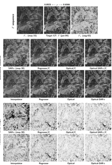
Further insight into the behavior of the compared methods can be gained by visual inspection of
369
some sample results. To this end we consider two target dates, June 4th and Aug 3rd, characterized
370
by significant temporal changes in spectral features with respect to the closest available dates. In
371
the first case, a high correlation exists with the previous date ρ = 0.8925 but not with the next 372
0.8925←−ρ−→0.6566
F
sequence
F−(may-15) Target GT:F(jun-04) F+(aug-03)
Estimated
feat
ur
es
SAR+ (may-30) Regressor/C Optical/C Optical-SAR+/C
Interpolator Regressor Optical Optical-SAR+
Absolute
erro
r
maps
SAR+ (may-30) Regressor/C Optical/C Optical-SAR+/C
Interpolator Regressor Optical Optical-SAR+
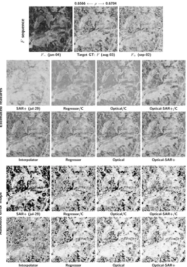
0.6566←−ρ−→0.6704
F
sequence
F−(jun-04) Target GT:F(aug-03) F+(sep-02)
Estimated
feat
ur
es
SAR+ (jul-29) Regressor/C Optical/C Optical-SAR+/C
Interpolator Regressor Optical Optical-SAR+
Absolute
erro
r
maps
SAR+ (jul-29) Regressor/C Optical/C Optical-SAR+/C
Interpolator Regressor Optical Optical-SAR+
These changes can be easily appreciated in the images, shown in the top row of Fig.4 and Fig.5,
374
respectively. In both figures, the results of most of the methods described before are reported,
375
omitting less informative cases for the sake of clarity. To allow easy interpretation of results, images
376
are organized for increasing complexity from left to right, with causal and non-causal versions shown
377
in the second and third row, respectively. As only exception, the first column shows results for SAR+
378
and non-causal interpolator. Moreover, in the last two rows, the corresponding absolute error images
379
are shown, suitably magnified, with the same stretching and reverse scale (white means no error) for
380
better visibility.
381
For jun-04, the estimation task is much simplified by the availability of the highly correlated
382
may-15 image. Since this precedes the target, causal estimators work almost as well as non-causal
383
ones. Moderate gradual improvements are observed going from left to right. Nonetheless,
384
by comparing the first (interpolator) and last (Optical-SAR+) non-causal solutions, a significant
385
accumulated improvement can be perceived, which becomes obvious in the error images. In this
386
case, even the SAR-only estimate is quite good, and the inclusion of SAR data (third to fourth column)
387
provides some improvements.
388
For the aug-03 image, the task is much harder, no good predictor images are available, especially
389
the previous image, 60 days old. In these conditions, there is clear improvement when going from
390
causal to non-causal methods, even more visible in the error images. Likewise, the left-to-right
391
improvements are very clear, both in the predicted images (compare for example the sharp estimate
392
of Optical-SAR+ with the much smoother output of the regressor) and in the error images, which
393
become generally brighter (smaller errors) and with fewer black patches. In this case, the SAR-only
394
estimate is very poor. Still, the inclusion of SAR data in the CNN-based estimators provides visible
395
improvements.
396
6. Conclusions 397
We have proposed and analyzed CNN-based methods for the estimation of spectral features
398
when optical data are missing. Several models have been considered, causal and non-causal,
399
single-sensor and joint-sensor, to take into account various situations of practical interest. Validation
400
has been conducted with reference to NDVI maps, using Sentinel-1 and Sentinel-2 time-series, but
401
the proposed framework is quite general, and can be readily extended to the estimation of other
402
spectral features. In all cases, the proposed methods outperform largely the conventional references,
403
especially in the presence of large temporal gaps. Besides proving the potential of deep learning
404
for remote sensing, experiments have shown that SAR images can be used to obtain a meaningful
405
estimate of spectral indexes when other sources of information are not available,
406
Such encouraging results suggest further investigation on these topics. First of all, very deep
407
CNN architectures should be tested, as they proved extremely successful in other fields. However,
408
this requires the creation of a large representative dataset for training. In addition, more advanced
409
deep learning solutions for generative problems should be considered, such as the recently proposed
410
Generative Adversarial Networks [56]. Finally, cross-sensor estimation from SAR data is a stimulating
411
research theme, and certainly deserves further study.
412
Supplementary Materials: Supplementary Materials: Software and implementation details will be made 413
available online athttp://www.grip.unina.it/to ensure full reproducibility. 414
Author Contributions: Author Contributions: G. Scarpa has proposed the research topic, written the paper, 415
and coordinated activities. M. Gargiulo and A. Mazza have equally contributed to develop and implement the 416
proposed solutions, and validate them experimentally. R. Gaetano has provided and preprocessed the dataset, 417
and contributed ideas from an application-oriented perspective. 418
Bibliography 419
1. Pohl, C.; Genderen, J.L.V. Review article Multisensor image fusion in remote sensing: Concepts, methods 420
2. Alparone, L.; Aiazzi, B.; Baronti, S.; Garzelli, A.; Nencini, F.; Selva, M. Multispectral and panchromatic 422
data fusion assessment without reference. Photogramm. Eng. Remote Sens.2008,74, 193–200. 423
3. Gaetano, R.; Amitrano, D.; Masi, G.; Poggi, G.; Ruello, G.; Verdoliva, L.; Scarpa, G. Exploration of 424
Multitemporal COSMO-SkyMed Data via Interactive Tree-Structured MRF Segmentation. IEEE Journal of 425
Selected Topics in Applied Earth Observations and Remote Sensing2014,7, 2763–2775. 426
4. Masi, G.; Cozzolino, D.; Verdoliva, L.; Scarpa, G. Pansharpening by Convolutional Neural Networks. 427
Remote Sensing2016,8, 594. 428
5. Palsson, F.; Sveinsson, J.R.; Ulfarsson, M.O. Multispectral and Hyperspectral Image Fusion Using a 429
3-D-Convolutional Neural Network. IEEE Geoscience and Remote Sensing Letters2017,14, 639–643. 430
6. Gaetano, R.; Moser, G.; Poggi, G.; Scarpa, G.; Serpico, S.B. Region-Based Classification of Multisensor 431
Optical-SAR Images. IGARSS 2008 - 2008 IEEE International Geoscience and Remote Sensing 432
Symposium, 2008, Vol. 4, pp. IV – 81–IV – 84. 433
7. Reiche, J.; Souza, C.M.; Hoekman, D.H.; Verbesselt, J.; Persaud, H.; Herold, M. Feature Level Fusion of 434
Multi-Temporal ALOS PALSAR and Landsat Data for Mapping and Monitoring of Tropical Deforestation 435
and Forest Degradation. IEEE Journal of Selected Topics in Applied Earth Observations and Remote Sensing 436
2013,6, 2159–2173. 437
8. Errico, A.; Angelino, C.V.; Cicala, L.; Persechino, G.; Ferrara, C.; Lega, M.; Vallario, A.; Parente, C.; 438
Masi, G.; Gaetano, R.; Scarpa, G.; Amitrano, D.; Ruello, G.; Verdoliva, L.; Poggi, G. Detection of 439
environmental hazards through the feature-based fusion of optical and SAR data: a case study in southern 440
Italy. International Journal of Remote Sensing2015,36, 3345–3367. 441
9. Das, M.; Ghosh, S.K. Deep-STEP: A Deep Learning Approach for Spatiotemporal Prediction of Remote 442
Sensing Data. IEEE Geosci. Remote Sensing Lett.2016,13, 1984–1988. 443
10. Sukawattanavijit, C.; Chen, J.; Zhang, H. GA-SVM Algorithm for Improving Land-Cover Classification 444
Using SAR and Optical Remote Sensing Data.IEEE Geoscience and Remote Sensing Letters2017,14, 284–288. 445
11. Ma, W.; Wen, Z.; Wu, Y.; Jiao, L.; Gong, M.; Zheng, Y.; Liu, L. Remote Sensing Image Registration With 446
Modified SIFT and Enhanced Feature Matching.IEEE Geoscience and Remote Sensing Letters2017,14, 3–7. 447
12. Clerici, N.; Calderón, C.A.V.; Posada, J.M. Fusion of Sentinel-1A and Sentinel-2A data for land cover 448
mapping: a case study in the lower Magdalena region, Colombia. Journal of Maps2017,13, 718–726. 449
13. Fauvel, M.; Chanussot, J.; Benediktsson, J.A. Decision Fusion for the Classification of Urban Remote 450
Sensing Images.IEEE Transactions on Geoscience and Remote Sensing2006,44, 2828–2838. 451
14. Márquez, C.; López, M.I.; Ruisánchez, I.; Callao, M.P. FT-Raman and NIR spectroscopy data fusion 452
strategy for multivariate qualitative analysis of food fraud. Talanta2016,161, 80 – 86. 453
15. Waske, B.; van der Linden, S. Classifying Multilevel Imagery From SAR and Optical Sensors by Decision 454
Fusion.IEEE Transactions on Geoscience and Remote Sensing2008,46, 1457–1466. 455
16. Reiche, J.; de Bruin, S.; Hoekman, D.; Verbesselt, J.; Herold, M. A Bayesian approach to combine 456
Landsat and ALOS PALSAR time series for near real-time deforestation detection. Remote Sensing2015, 457
7, 4973–4996. 458
17. Du, P.; Liu, S.; Xia, J.; Zhao, Y. Information fusion techniques for change detection from multi-temporal 459
remote sensing images.Information Fusion2013,14, 19 – 27. 460
18. Masi, G.; Cozzolino, D.; Verdoliva, L.; Scarpa, G. CNN-based Pansharpening of Multi-Resolution 461
Remote-Sensing Images. Joint Urban Remote Sensing Event 2017; , 2017. 462
19. Scarpa, G.; Vitale, S.; Cozzolino, D. Target-adaptive CNN-based pansharpening. ArXiv e-prints2017, 463
[arXiv:cs.CV/1709.06054]. 464
20. Gaetano, R.; Masi, G.; Poggi, G.; Verdoliva, L.; G., S. Marker controlled watershed based segmentation of 465
multi-resolution remote sensing images.IEEE Trans. Geosci. Remote Sens.2015,53, 1987–3004. 466
21. Du, Y.; Zhang, Y.; Ling, F.; Wang, Q.; Li, W.; Li, X. Water Bodies’ Mapping from Sentinel-2 Imagery with 467
Modified Normalized Difference Water Index at 10-m Spatial Resolution Produced by Sharpening the 468
SWIR Band.Remote Sensing2016,8, 354. 469
22. Zanetti, M.; Bruzzone, L. A Theoretical Framework for Change Detection Based on a Compound 470
Multiclass Statistical Model of the Difference Image. IEEE Transactions on Geoscience and Remote Sensing 471
2017. 472
23. Liu, W.; Yang, J.; Zhao, J.; Yang, L. A Novel Method of Unsupervised Change Detection Using 473
24. Han, Y.; Bovolo, F.; Bruzzone, L. Segmentation-Based Fine Registration of Very High Resolution 475
Multitemporal Images.IEEE Transactions on Geoscience and Remote Sensing2017,55, 2884–2897. 476
25. Chierchia, G.; Gheche, M.E.; Scarpa, G.; Verdoliva, L. Multitemporal SAR Image Despeckling Based on 477
Block-Matching and Collaborative Filtering. IEEE Transactions on Geoscience and Remote Sensing2017, 478
55, 5467–5480. 479
26. Maity, S.; Patnaik, C.; Chakraborty, M.; Panigrahy, S. Analysis of temporal backscattering of cotton crops 480
using a semiempirical model. IEEE Transactions on Geoscience and Remote Sensing2004,42, 577–587. 481
27. Manninen, T.; Stenberg, P.; Rautiainen, M.; Voipio, P. Leaf Area Index Estimation of Boreal and Subarctic 482
Forests Using VV/HH ENVISAT/ASAR Data of Various Swaths. IEEE Transactions on Geoscience and 483
Remote Sensing2013,51, 3899–3909. 484
28. Borges, E.F.; Sano, E.E.; Medrado, E. Radiometric quality and performance of TIMESAT for smoothing 485
moderate resolution imaging spectroradiometer enhanced vegetation index time series from western 486
Bahia State, Brazil.Journal of Applied Remote Sensing2014,8, 083580–083580. 487
29. Zhang, H.; Lin, H.; Li, Y. Impacts of Feature Normalization on Optical and SAR Data Fusion for Land 488
Use/Land Cover Classification. IEEE Geoscience and Remote Sensing Letters2015,12, 1061–1065. 489
30. Man, Q.; Dong, P.; Guo, H. Pixel-and feature-level fusion of hyperspectral and lidar data for urban 490
land-use classification. International Journal of Remote Sensing2015,36, 1618–1644. 491
31. Lu, M.; Chen, B.; Liao, X.; Yue, T.; Yue, H.; Ren, S.; Li, X.; Nie, Z.; Xu, B. Forest Types Classification Based 492
on Multi-Source Data Fusion.Remote Sensing2017,9, 1153. 493
32. Pal, S.K.; Majumdar, T.J.; Bhattacharya, A.K. ERS-2 SAR and IRS-1C LISS III data fusion: A PCA approach 494
to improve remote sensing based geological interpretation. ISPRS Journal of Photogrammetry and Remote 495
Sensing2007,61, 281–297. 496
33. Bolten, J.D.; Lakshmi, V.; Njoku, E.G. Soil moisture retrieval using the passive/active L- and S-band 497
radar/radiometer.IEEE Transactions on Geoscience and Remote Sensing2003,41, 2792–2801. 498
34. Baghdadi, N.N.; Hajj, M.E.; Zribi, M.; Fayad, I. Coupling SAR C-Band and Optical Data for Soil Moisture 499
and Leaf Area Index Retrieval Over Irrigated Grasslands. IEEE Journal of Selected Topics in Applied Earth 500
Observations and Remote Sensing2016,9, 1229–1243. 501
35. Santi, E.; Paloscia, S.; Pettinato, S.; Entekhabi, D.; Alemohammad, S.H.; Konings, A.G. Integration of 502
passive and active microwave data from SMAP, AMSR2 and Sentinel-1 for Soil Moisture monitoring. 503
2016 IEEE International Geoscience and Remote Sensing Symposium (IGARSS), 2016, pp. 5252–5255. 504
36. Addabbo, P.; Focareta, M.; Marcuccio, S.; Votto, C.; Ullo, S.L. Land cover classification and monitoring 505
through multisensor image and data combination. 2016 IEEE International Geoscience and Remote 506
Sensing Symposium (IGARSS), 2016, pp. 902–905. 507
37. Jelének, J.; Kopaˇcková, V.; Koucká, L.; Mišurec, J. Testing a Modified PCA-Based Sharpening Approach 508
for Image Fusion.Remote Sensing2016,8, 794. 509
38. Bisquert, M.; Bordogna, G.; Boschetti, M.; Poncelet, P.; Teisseire, M. Soft Fusion of heterogeneous image 510
time series. International Conference on Information Processing and Management of Uncertainty in 511
Knowledge-Based Systems. Springer, 2014, pp. 67–76. 512
39. Moran, M.S.; Hymer, D.C.; Qi, J.; Sano, E.E. Soil moisture evaluation using multi-temporal synthetic 513
aperture radar (SAR) in semiarid rangeland.Agricultural and Forest Meteorology2000,105, 69 – 80. 514
40. Wang, Q.; Blackburn, G.A.; Onojeghuo, A.O.; Dash, J.; Zhou, L.; Zhang, Y.; Atkinson, P.M. Fusion 515
of Landsat 8 OLI and Sentinel-2 MSI Data. IEEE Transactions on Geoscience and Remote Sensing2017, 516
55, 3885–3899. 517
41. Haas, J.; Ban, Y. Sentinel-1A SAR and sentinel-2A MSI data fusion for urban ecosystem service mapping. 518
Remote Sensing Applications: Society and Environment2017,8, 41 – 53. 519
42. Inglada, J.; Arias, M.; Tardy, B.; Hagolle, O.; Valero, S.; Morin, D.; Dedieu, G.; Sepulcre, G.; Bontemps, S.; 520
Defourny, P.; Koetz, B. Assessment of an Operational System for Crop Type Map Production Using High 521
Temporal and Spatial Resolution Satellite Optical Imagery. Remote Sensing2015,7, 12356–12379. 522
43. ESA. ESA Sentinel Application Platform (SNAP) software. http://step.esa.int/main/toolboxes/snap, 523
(accessed on 13 December 2017). 524
45. Hagolle, O.; Huc, M.; Villa Pascual, D.; Dedieu, G. A Multi-Temporal and Multi-Spectral Method to 526
Estimate Aerosol Optical Thickness over Land, for the Atmospheric Correction of FormoSat-2, LandSat, 527
VENµS and Sentinel-2 Images. Remote Sensing2015,7, 2668–2691. 528
46. Zhang, K.; Zuo, W.; Chen, Y.; Meng, D.; Zhang, L. Beyond a Gaussian Denoiser: Residual Learning of 529
Deep CNN for Image Denoising. IEEE Transactions on Image Processing2017,26, 3142–3155. 530
47. Dong, C.; Loy, C.; He, K.; Tang, X. Image Super-Resolution Using Deep Convolutional Networks. IEEE 531
Transactions on Pattern Analysis and Machine Intelligence2016,38, 295–307. 532
48. Long, J.; Shelhamer, E.; Darrell, T. Fully convolutional networks for semantic segmentation. Computer 533
Vision and Pattern Recognition (CVPR), 2015 IEEE Conference on, 2015, pp. 3431–3440. 534
49. Zhang, N.; Donahue, J.; Girshick, R.; Darrell, T. Part-Based R-CNNs for Fine-Grained Category Detection. 535
Proceedings of European Conference on Computer Vision, 2014. 536
50. Krizhevsky, A.; Sutskever, I.; Hinton, G.E. Imagenet classification with deep convolutional neural 537
networks. Advances in Neural Information Processing Systems, 2012, pp. 1106–1114. 538
51. Jiao, L.; Liang, M.; Chen, H.; Yang, S.; Liu, H.; Cao, X. Deep Fully Convolutional Network-Based Spatial 539
Distribution Prediction for Hyperspectral Image Classification.IEEE Transactions on Geoscience and Remote 540
Sensing2017,55, 5585–5599. 541
52. Goodfellow, I.; Bengio, Y.; Courville, A. Deep Learning; MIT Press, 2016. http://www.deeplearningbook. 542
org. 543
53. Sutskever, I.; Martens, J.; Dahl, G.E.; Hinton, G.E. On the importance of initialization and momentum in 544
deep learning. ICML (3)2013,28, 1139–1147. 545
54. Cire¸san, D.C.; Gambardella, L.M.; Giusti, A.; Schmidhuber, J. Deep neural networks segment neuronal 546
membranes in electron microscopy images. In NIPS, 2012, pp. 2852–2860. 547
55. Orfeo Toolbox: Temporal gap-filling. http://tully.ups-tlse.fr/jordi/temporalgapfilling, (accessed on 13 548
December 2017). 549
56. Goodfellow, I.; Pouget-Abadie, J.; Mirza, M.; Xu, B.; Warde-Farley, D.; Ozair, S.; Courville, A.; Bengio, Y. 550

![Table 3. Correlation index, ρ ∈ [−1, 1].](https://thumb-us.123doks.com/thumbv2/123dok_us/1079394.1608695/10.595.111.484.110.271/table-correlation-index-r.webp)
![Table 4. Peak signal-to-noise ratio (PSNR) [dB].](https://thumb-us.123doks.com/thumbv2/123dok_us/1079394.1608695/11.595.113.485.306.467/table-peak-signal-to-noise-ratio-psnr-db.webp)