Image-Based Multi-Target Tracking Through
Multi-Bernoulli Filtering with Interactive Likelihoods
Anthony Hoak, Henry Medeiros * and Richard J. Povinelli
Department of Electrical & Computer Engineering, Marquette University, 1551 W. Wisconsin Ave., Milwaukee, WI 53233, USA; [email protected] (A.H.); [email protected] (R.J.P.)
* Correspondence: [email protected]; Tel.: +1-414-288-6186
Abstract: We develop an interactive likelihood (ILH) for sequential Monte-Carlo (SMC) methods for image-based multiple target tracking applications. The purpose of the ILH is to improve tracking accuracy by reducing the need for data association. In addition, we integrate a recently developed deep neural network for pedestrian detection along with the ILH with a multi-Bernoulli filter. We evaluate the performance of the multi-Bernoulli filter with the ILH and the pedestrian detector in a number of publicly available datasets (2003 PETS INMOVE, AFL, and TUD-Stadtmitte) using standard, well-known multi-target tracking metrics (OSPA and CLEAR MOT). In all datasets, the ILH term increases the tracking accuracy of the multi-Bernoulli filter.
Keywords:multi-target tracking; multi-Bernoulli filter; sequential Monte-Carlo
1. Introduction
Multi-target tracking (MTT) is a well-researched problem, with a history going back over50years [1], however, it remains an open research problem [2,3]. It has many applications including aviation [4] and air traffic control [5], ballistic missile defense [6,7], smart surveillance [8,9], robotics [10], and autonomous vehicles [11–15]. The goal of MTT is to simultaneously estimate both the number of targets and their states (position, size, velocity, etc.) through time [16]. This can be a difficult task for a number of different reasons; to name just a select few of these challenges: 1) mathematically consistent ways of defining and using estimation error; 2) mathematically modeling targets entering and leaving the scene (target births and deaths); 3) the task of data association (associating targets with correct measurements as well as associating targets temporally); and 4) robustness to different and dynamic scenarios.
In image-based tracking, measurements are in the form of individual image frames and the objective is to track the targets and their states through the image sequence. It is often the case that multiple measurement observations are made within a given image frame and it is necessary to associate these measurements with targets or tracks1 (tracks are defined by Risticet al. [16] as a “labeled temporal sequence of state estimates associated with the same target”).
In this paper, an interactive likelihood (ILH) for the multi-Bernoulli filter (MBF)2 is developed and evaluated. The purpose of the ILH is to reduce the need for data association, addressing challenge3. It is based entirely within the Bayesian random finite set (RFS) framework and therefore does not require any external data association mechanism(s). The proposed approach is a novel method for addressing the fundamental data association issue in the field of multi-target tracking [4]. The Bayesian-RFS framework simultaneously handles challenges1and2very elegantly, and much progress has been made in recent years to also address challenge3 using this framework in a mathematically rigorous way through the labeled multi-Bernoulli filter and its variants [17–22]. Our work corresponds to another important step in that direction.
In order to address challenge4, a state-of-the-art deep neural network for pedestrian detection is integrated into the MBF with the ILH. To the best of our knowledge, there has been no work on integrating deep networks in a track-before-detect Bayesian-RFS framework. Because deep networks achieve such promising results in
1 The terms ‘tracks’ and ‘trajectories’ are used interchangeably in this article.
object and pedestrian detection and the lack of existing research in using these detectors with RFS approaches, there is substantial unexplored potential in the combination of these two state-of-the-art techniques.
Specifically, the main contributions presented in this paper are as follows:
1. a novel interactive likelihood (ILH) method for sequential Monte-Carlo (SMC) image-based trackers that can be computed non-iteratively to preclude the tracker from sampling from areas that belong to different targets;
2. this interactive likelihood method is integrated with the multi-Bernoulli filter, a state-of-the-art RFS tracker, which is referred to as MBFILH;
3. the deep learning technique for pedestrian detection proposed in [23] is combined with the MBFILH; and 4. an extensive evaluation is carried out using several publicly available datasets and standard evaluation
metrics.
The rest of this paper is organized as follows: Section 2 discusses related works, including a brief description of common multi-target tracking algorithms as well as highlighting recent trends. In Section3, we present necessary background information, notation, and definitions. We develop our ILH in Section4. In Section5we evaluate the ILH in a number of different datasets, report numerical results, and provide a brief discussion of these results. Finally, in Section6we briefly summarize our contribution.
2. Related Work
In this section we present a general discussion of multi-target tracking including standard techniques, challenges, and also identify a trend in the current research within the multi-target tracking community.
2.1. Common Multi-Target Tracking Algorithms
Many different MTT methods have been proposed over the years, but the most mature and most common algorithms are the joint probabilistic data association filter (JPDAF) [24] and the multiple hypothesis tracking (MHT) method [4]. In the last decade [1], there has been substantial research in the use of random finite sets within a Bayesian framework for multi-target tracking [25–32]. One benefit to RFS-based approaches is that they have mathematically consistent and rigorous ways for handling estimation error and target births and deaths. In other words, they are well equipped to handle challenges numbers1and2listed in the first paragraph of Section1. In the last two years, there has been a resurgence of detection-based approaches, including new variations of the more mature multi-target tracking algorithms, for example a revisiting of the JPDAF [33]. Most recently, due to the vast amount of research on (deep) neural networks for object and pedestrian detection [23,34–37,37–41], track-by-detection multi-target tracking approaches are starting to be proposed that make use of these stat-of-the-art detectors [42].
The process of associating measurements with appropriate targets or tracks is known as data association. Historically it is one of the major challenges in multi-target tracking [4] and is still an active research topic [43–45]. It is desirable for targets to remain separated within the image and for no occlusions to take place; however, this is often not the case. For example, in sport player tracking situations, targets often are in close proximity and occlusions are frequent. This type of situation can lead to numerous, ambiguous measurements, where data association becomes especially important. If the data association process is not handled adequately, target tracks or labels may be switched or dropped entirely, resulting in overall tracking inaccuracy.
The two classical multi-target tracking algorithms, JPDAF and MHT, have internal mechanisms to accomplish the data association task. However, traditional RFS approaches do not have such mechanisms in place and therefore often require an additional layer of complexity external to the RFS framework in order to perform data association. For example, in [25], a graph theoretical approach (based on the work of Shafique and Shah in [45]) is used in conjunction with a multi-Bernoulli filter. The significant recent contributions on the labeled multi-Bernoulli filter correspond to additional attempts to overcome this limitation [17–22].
association, however, in practice, these trackers need to be implemented using Monte-Carlo approaches and the sampling process introduces confusion that may cause incorrect associations. Hence, in practice data association is strictly necessary for multi-target tracking, even when RFS approaches are employed, and is also still one of the most limiting factors.
To address this fundamental issue, an interactive likelihood for the multi-Bernoulli filter is presented. The interactive likelihood technique exploits the spatial information that exists in any given image observation and reduces the need for data association. It works by modifying the sequential Monte Carlo sampling process so that the spatial probability distributions of nearby similar targets do not overlap. As a result, it reduces the confusion among these targets and hence avoids estimation errors in these challenging scenarios.
2.2. Current Trends
Most multi-target tracking algorithms can also be classified as either track-by-detection or track-before-detection. Track-by-detection algorithms use post-processed data, that is, the raw sensor measurements have had some kind of thresholding performed [47]. There is a vast amount of work currently being done on developing and evaluating new algorithms (since 2015) that fall into the former category [3,48–52]. In track-by-detection approaches, there are often separate techniques for detection and data association. In these approaches, detections are typically obtained by a scanning algorithm that searches the entire image and determines where targets are likely to be. These detections are then processed by a separate algorithm for association. This effectively splits the multi-target tracking problem into two separate problems: detection and association. In fact, in the most recently proposed multi-target tracking benchmarks [53] and [54], it is encouraged to use ‘standard’ detections to remove entirely the problem of detection and focus completely on association. This means that new multi-target tracking methods can be proposed, which are incapable of producing measurements from an image, and therefore do not really even need to process images at all, but must only be able to use these standard detections. This allows for relatively quick evaluations in large datasets with large image sizes. While this paradigm is beneficial for the sake of fairly comparing all track-by-detection approaches, it has a number of other effects: 1) it removes all image processing from the task and thus, it is no longer a computer vision problem; 2) it becomes difficult for sequential Monte-Carlo approaches to be included in the benchmarks as Monte-Carlo evaluations are necessary and numerous trials must be performed taking significantly longer in large datasets than using standard, precomputed detections, 3) all track-before-detection approaches are also at a disadvantage as they solve both the detection and tracking problems simultaneously, adding more opportunities for error and, 4) it assumes that detectors have plateaued in performance, which may inadvertently reduce the amount of research to develop new and higher performing detectors.
In situations in which target detection itself is challenging, such as in scenarios with substantial clutter, track-before-detect methods tend to perform significantly better [55–57]. The contribution presented in this paper, hence, falls into the second category, track-before-detection, in which there are no scanning or searching schemes involved, and detections are not strictly necessary. This method is also considered ‘online’, as new estimates about the current multi-target state are available at each time instant.
3. Method
In this section we provide some necessary background for presenting our method. We briefly discuss the image-based multi-Bernoulli filter, its corresponding Bayes’ recursion, and describe a particle filter implementation.
3.1. Image-Based Multi-Bernoulli Filter
The interactive likelihood presented in this paper is constructed within the multi-Bernoulli filter presented by Hoseinnezhadet al. in [25]. Therefore, the notation used for the multi-target Bayes’ and multi-Bernoulli filter will be similar. Prior to describing the interactive likelihood and its development, it is necessary to establish a number of definitions. A single image ofmtotal pixels is represented by a one dimensional vector
y=hy0 · · · ym
iT
For a single image within an image sequence, let the number of targets benand their states bex1,x2,· · ·xn. In
this paper, the state of each targetxiconsists of its horizontaluand verticalvcoordinates in the image as well
as its heighthand widthwsuch that
xi =
h
u v h wiT. (2)
Then the multi-target state is represented as a finite set
X={x1,x2,· · ·xn}. (3)
The defining feature of the multi-Bernoulli filter is the multi-Bernoulli RFS, which is a union ofMindependent Bernoulli RFSs. The probability density of a Bernoulli RFSX(i)is (see [29,58] for details regarding Bernoulli and multi-Bernoulli RFSs)
π(X(i)) = (
1−r, ifX(i)=∅
r·p(·), ifX(i)={xi},
(4)
wherer is the probability of existence forxi, the only element of Xif it is non-empty, and xi is distributed
according to the probability densityp(·).X(i)has the probability1−rof being empty. Then a multi-Bernoulli RFSXis the union ofMindependent Bernoulli RFSsX(i)
X=
M
[
i=1
X(i) (5)
and is fully characterized by the parameter set{(r(i),p(i)(·))}M i=1[25].
3.2. Bayes’ Recursion
Detailed discussions of the Bayes’ recursion and the multi-Bernoulli filter can be found in [25–28,30]. Only the essential information will be listed here. For a given multi-target stateXand image sequencey1:k−1, the multi-target Bayes’ filter computes the predicted stateπk|k−1(Xk|y1:k−1)by propagating the multi-target posterior πk−1(·|y1:k−1) from time step k−1 to k through the multi-target transition density fk|k−1(·|·). Once a measurement is available, the posterior at time k, πk(Xk|y1:k), is computed using the multi-target
likelihood function g(·|·) (see Mahler’s FISST [59,60] for more detailed information on the set integrals required to perform these steps). The Bayes’ recursion is, in general, intractable [27–30,58] and therefore approximations are necessary. We adopt the commonly-used multi-target transition density discussed in [25,27], such that at timek−1, the elementsxk−1of the multi-target stateXk−1either continue to exist at timekwith probabilitypS,k(xk−1)and transition to statexkwith probability densityfk|k−1(xk|xk−1)or die with probability
1−pS,k(xk−1). The behavior of a target with statexk−1at timek−1can then be modeled bySk|k−1(xk−1), which are the Bernoulli RFSs corresponding to each target that survived at time instantk[27]. At timekthe multi-target stateXkis then
Xk=
[
xk−1∈Xk−1
Sk|k−1(xk−1)∪Γk. (6)
The RFS Γk = {(r(Γi,)k,p(Γi,)k(·))}MΓ,k
i=1 contains all of the targets born at timek. The likelihood of an image observationygiven the multi-target stateXis
g(y|X) =
n
∏
i=1
gf(yxi), (7)
3.3. Likelihood Functions
We first employ the same likelihood functiongf(yxi)as [25] and more detailed information can be found there regarding how it is constructed. For the scope of this paper, it is sufficient to say that it is based on hue-saturation-value (HSV) histograms and the training data consists ofntrain =850references histograms to
which target histograms are compared. It has the form
gf(vi) =
ζ ntrainhN
ntrain
∑
j=1
κ d(v
i,v∗j)
h
, (8)
whereζis a normalization constant, vi is the target histogram vector of y,{v∗j} ntrain
j=1 is the set of reference histograms,κ(·)is a Gaussian kernel function,h is the kernel bandwidth, andNis the number of histogram bins. The difference between histograms is measured using the Bhattacharyya distance, given by
d(vi,v∗j) =
1−
N
∑
r=1
q
v∗j(r)vi(r)
1/2
. (9)
We consider a second, simple but more general likelihood function based on the pedestrian detector presented in [23]
gf(yxi) =γPD(yxi)
2, (10)
wherePD(yxi)is the output of the pedestrian detector for the image observationyxiandγis a scalar coefficient. More information about the pedestrian detector will be presented in Section4.1.
3.4. Particle Filter Implementation
RFS filters (including the multi-Bernoulli) are often implemented using sequential Monte-Carlo (SMC) methods such as the particle filter [25,26,28,30,31,61]. We use the particle filter implementation used by Hoseinnezhad et al. in [25], which is similar to those used in [28] and [27]. In order to translate the multi-Bernoulli recursion to a particle filter implementation, let the proposal densities q(ki)(·|xk−1,yk) and
b(ki)(·|yk)be known and the probability densityp(ki−)1(·)be given by a set of weighted samples (particles)
p(ki−)1(x) =
L(i)k−1
∑
j=1
w(ki−,j)1δ
x(ik−,j)1(x). (11)
Also, suppose that at time k−1 the multi-target multi-Bernoulli posterior πk−1 is known, then the multi-Bernoulli parameters for the predicted target state can be calculated as follows:
r(ki|)k−1=r(ki−)1
L(i)k−1
∑
j=1
w(ki−,j)1pS,k(x
(i,j)
k−1). (12)
p(ki|)k−1(x) =
L(i)k−1
∑
j=1
˜ w(ki|,kj)−1δ
xk(i|,kj)−1(x). (13)
rΓ(i,)k= birth model parameter. (14)
p(Γi,)k(x) =
L(i)Γ,k
∑
j=1
˜ w(Γi,,kj)δ
where
x(ki|,kj−)1∼q(ki)(·|xk(i−,j1),yk),forj=1,· · ·,L(ki|)k−1, (16)
w(ki|,kj)−1= w
(i,j)
k−1fk|k−1(x (i,j)
k|k−1|x (i,j)
k−1)pS,k(x (i,j)
k−1)
qk(i)(xk(i|k,j)−1|x(ki−,j)1)
, (17)
˜
w(ki|,kj)−1= w
(i,j)
k|k−1
∑L
(i) k|k−1
j=1 w (i,j)
k|k−1
, (18)
xΓ(i,,kj)∼b(ki)(·|yk)forj=1,· · ·,L(Γi,)k, (19)
w(Γi,,kj)= pΓ,k(x
(i,j)
Γ,k )
bk(i)(xΓ(i,,kj)|yk)
, (20)
˜
w(Γi,,kj)= w
(i,j)
Γ,k
∑L
(i) Γ,k
j=1w (i,j)
Γ,k
. (21)
Once the multi-Bernoulli parameters have been predicted, that is, πk|k−1 = {(rk(i|)k−1,p (i)
k|k−1(·))}
Mk|k−1
i=1 is known, the updated multi-Bernoulli parameters can be computed as follows:
r(ki)= r
(i)
k|k−1$ (i)
k
1−r(ki|)k−1+rk(i|)k−1$(ki)
, (22)
p(ki)= 1 $(ki)
L(i)k|k−1
∑
j=1
w(ki|,kj−)1gyk(x (i,j)
k|k−1)δx(ik|,kj)−1(x), (23)
$(ki)=
L(i)k|k−1
∑
j=1
w(ki|,kj−)1gyk(x(ki|,kj)−1). (24)
4. Interactive likelihood
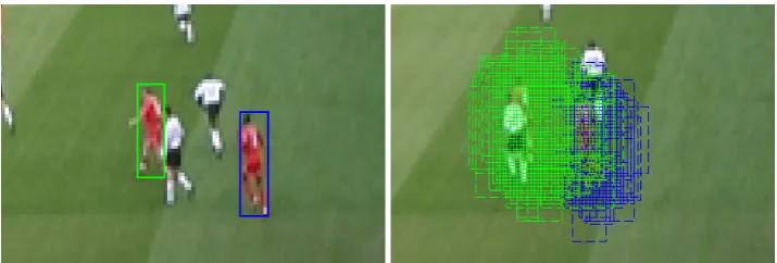
Figure 1.These two images illustrate the sensitivity of SMC methods to clutter. Left: Two targets tracked by a particle filter implementation of a multi-Bernoulli filter. The solid green and blue rectangles represent the estimated positions of the targets. Right: The same targets being tracked while particles are visible. Dashed rectangles represent the particles. Note how some particles of the target on the left (green) overlap and sample the target on the right (blue) (original images obtained from the2003PETS INMOVE dataset).
Figure 2.The distance between particlex(i,j)of targetx(i)and particlex(m,`)of targetx(m). The green and blue rectangles represent the particles associated with the two targets. The centers of the estimated target positions are represented by the black circles.
causes the estimated position to change, which in turn changes the particle positions. This iterative estimation can be avoided by using particle distances directly as proposed here. The first step in constructing the interactive likelihood is to associate particles with targets. This requires augmenting the state of the target with a unique label. Particles are then associated with a label and distances can then be computed for particles associated with a given label to the particles associated with all other labels. The distance between the jth particle of target
x(i), denotedx(i,j), and the`thparticle of targetx(m), denotedx(m,`), is calculated in the image plane using the Euclidean distance
d(j,i`,m)(x(i,j),x(m,`)) =
q
(u(i,j)−u(m,`))2+ (v(i,j)−v(m,`))2, (25)
where u(·) and v(·) are respectively the horizontal and vertical pixel coordinates of the centroid of the corresponding particle rectangle (see Fig. 2for an illustration of this distance). We intentionally refrain from using the4D distance (that is, we do not include the width and height of the target) because we want to avoid confusion between target samples regardless of the relative target sizes. It should be noted that the case where
i = mcorresponds to the distance from a given target to itself, and therefore does not need to be calculated. This distance is then used within the interactive likelihood weighting function.
Suppose that between the prediction step at timek−1and the update step to timek, the cardinality of the multi-target state Xis M. Let the number of particles associated with a given targetx(i) be L(i). The
0 50 100 150 200 250 300 350 400 450 500 0 0.2 0.4 0.6 0.8 1 Distance Interactive Likelihood
ζ = 0.1
ζ = 0.5
ζ = 0.9
(a)
0 50 100 150 200 250 300 350 400 450 500
0 0.2 0.4 0.6 0.8 1 Distance Interactive Likelihood
σ = 50
σ = 250
σ = 500
(b)
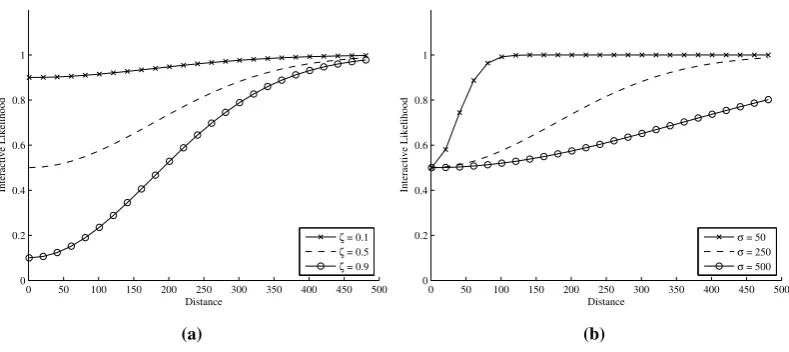
Figure 3. a) Effect of changingζwhile keepingσ =250. Thex-axis represents distance (in pixels) and the
y-axis is the corresponding interactive likelihood function value. The top, middle, and lower lines correspond to
ζvalues of0.1,0.5, and0.9, respectively. b) Effect of changingσwhile keepingζ=0.5. Thex-axis represents distance (in pixels) and they-axis is the corresponding interactive likelihood function value. The top, middle, and lower lines correspond toσvalues of50,250, and500, respectively.
weighting function (note that the time subscript is dropped for notational convenience, but these calculations must be performed during each time step)
α(i,j)(x(i,j)) =
M
∏
m=1
m6=i L(m)
∏
`=1
1−ζe
− d(j,i`,m)(x(i,j),x(m,`))2
σ2 . (26)
Bothζ andσ can be considered tuning parameters. The threshold at which the interactive likelihood starts to influence particle weights is determined byσ; it defines what is ‘close enough proximity’ and corresponds to the (pixel) distance at which targets start to influence one another. The higher the value of σ, the greater the distance of the influence of the interactive likelihood. The intensity of the influence is determined byζ. These two parameters can be adjusted to obtain the desired particle interaction behavior for a given application. Fig. 3aand Fig. 3billustrate, in a2D example, how changing bothσ andζ affect the interactive likelihood magnitude. The interactive likelihood termα(i,j)can then be integrated into the particle filter update steps Eq. (23) and Eq. (24) by simply multiplying the standard likelihoodgyk(x
(i,j)
k|k−1)term by the interactive likelihood termα(i,j)(xk(i|,kj−)1),
p(ki)= 1 $(ki)
L(i)k|k−1
∑
j=1
w(ki|,kj)−1gyk(x (i,j)
k|k−1)·α
(i,j)(x(i,j)
k|k−1)δx(ik|,kj)−1(x), (27)
$(ki)=
L(i)k|k−1
∑
j=1
w(ki|,kj−)1gyk(x(ki|,kj−)1)α(i,j)(xk(i|,kj)−1). (28)
It should be noted that Eq. (22) also changes appropriately.
4.1. Deep Learning for Pedestrian Detection
Channel 1 Channel 2 Channel 3
28 28 28
84 Y channel of YUV converted image 84 84
Y 42x14
U 42x14
V 42x14
Zeros 42x14
Y edges 42x14
U edges 42x14
Max edges 42x14 V edges
42x14
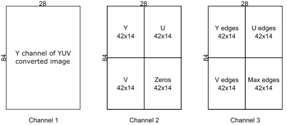
Figure 4.Composition of input channels to the pedestrian detector.
reasoning and classification layer. The2009Caltech pedestrian detection dataset [65] was used for the training of the network.
As mentioned in Section3.2, we use the pedestrian detector as a likelihood function and therefore the algorithm still retains the track-before-detect characteristic. This is accomplished by feeding the network with each particle associated with a given target and using the output of the network straightforwardly as the likelihood of that particle. Therefore Eqs.27and28remain the same; however, the likelihood function is now given by Eq. (10) instead of Eq. (8). We refer to the MBF and MBFILH with the pedestrian detector (PD) likelihood function as MBF PD and MBFILH PD, respectively.
In order to use the pedestrian detector, it is necessary to preprocess the input data (the random sized particles/samples from the multi-Bernoulli filter shown as dashed-line rectangles in Fig.1). Each particle is first converted to YUV color space and resized to84×28, hence, all three input channels require an image of overall size84×28. For channel two, the overall dimensions of84×28are achieved by concatenating three images of size42×14and padding with zeros. For channel three, four42×14images are concatenated. Explicitly, the input to each of the three channels is as follows:
1. Channel 1 input = the Y channel of the resized (to84×28) YUV converted image.
2. Channel 2 input = the Y, U, and V channels of the84×28image resized to42×14, concatenated, and zero padded to achieve the overall dimensions of84×28.
3. Channel 3 input = three edge maps (horizontal and vertical) obtained from each channel of the YUV converted image using a Sobel edge detector, resized to be 42×14, and concatenated along with the maximum values of these three edge maps into an image of overall size84×28.
See Fig. 4for further clarification. It should be noted that the pedestrian detector deep network uses a binary softmax function and therefore returns two values: the first value is the probability of the image window containing a pedestrian and the second is the probability that it does not. We only use the former and simply ignore the latter.
As with most likelihood functions, the pedestrian detector-based likelihood function requires tuning in order to achieve desired behavior. However, it only requires adjustment of one parameterγ. Adjusting this parameter is straightforward and relatively simple. Higher values forγresult in higher likelihood values for all observations and lower values result in lower likelihood values.
5. Experiments and Results
1. 2003 PETS INMOVE:3 In this dataset, the performance of the multi-Bernoulli filter without (MBF) the ILH, with the ILH (MBFILH), an implementation of the multiple hypothesis tracking (MHT) method [66], the multi-Bernoulli filter without the ILH and with a fixed target size (MBF FS), and the multi-Bernoulli filter with the ILH with a fixed target size (MBFILH FS) is evaluated; the HSV-based likelihood function in Eq. (8) is used for all RFS filter configurations (MBF, MBFILH, MBF FS, and MBFILH FS) within this dataset.
• Empirically determined interactive likelihood parameters:ζ=0.15andσ=5
2. Australian Rules Football League (AFL) [67]: In this dataset, the MBF and the MBFILH filter configurations use the likelihood function in Eq. (8).
• Empirically determined interactive likelihood parameters: ζ = 0.15 and σ = 5 in reduced resolution images andζ=0.15andσ=10in full resolution images
3. TUD-Stadtmitte [68]: in this dataset, the pedestrian detector-based likelihood function in Eq. (10) is used with the multi-Bernoulli filter without the ILH (MBF PD) and with the ILH (MBFILH PD).
• Empirically determined interactive likelihood parameters:ζ=0.45andσ=150
• Empirically determined pedestrian detector parameters:γ=0.30
It is an intentional choice tonotuse the most recent benchmarks [53] and [54] because the framework (using standard detections) is not well suited for techniques that use SMC implementations and precludes track-before-detect methods in general.
5.1. 2003 PETS INMOVE
We first present results in the 2003 PETS INMOVE dataset. This dataset consists of 2500frames of a soccer match. We use reduced resolution images (320×240) from the dataset to perform the evaluation. This illustrates the flexibility of our approach as it is able to perform well in low signal-to-noise ratio (SNR) situations. Using reduced resolution also slightly reduces computation time.
Our implementation of the multi-Bernoulli filter is based on the source code kindly provided by the authors of [25]. Except for a few minor changes in the birth model parameters and color histogram computation, both implementations are identical. All trackers in this experiment are set up to track only the players on the red team (Liverpool) in the 2003 PETS INMOVE dataset. Within the RFS filters, targets are modeled as rectangular blobs and have states corresponding to Eq. (2) with theuandvposition of the target along with the widthw
and heighthof the target’s bounding box. Because the implementation of the MHT in [66] does not estimate target size, we also evaluate the multi-Bernoulli filters with fixed target size.
In order to show that the proposed interactive likelihood is able to almost entirely eliminate the need for data association, we compare our method to the multi-Bernoulli filter proposed by Hoseinnezhadet al. in [25] without the data association algorithm [45] in place and to the MHT implementation of Antuneset al. [66]. Given the stochastic nature of the algorithms, a Monte-Carlo evaluation was necessary. Specifically, we carried out20experimental trials for each filter configuration (MBF, MBFILH, MHT, MBF FS, and MBFILH FS). We initialized the multi-Bernoulli filters with the targets in the first frame in order to achieve a fair comparison to the window scanning detector in the implementation of the MHT filter. Each trial progressed through all2500 frames of the dataset.
The optimal sub-pattern assignment (OSPA) [69] and CLEAR MOT (classification of events, activities and relationships for multi-object trackers) [70] metrics were used to obtain quantitative results from each filter configuration. In the OSPA evaluation, a cutoff parameter ofc =100was used along with an order parameter ofp =1. See [69] for detailed information on the OSPA metric along with an interpretation of the parameters
candp. Briefly,ccorresponds to the maximum allowed distance for two tracks to be considered comparable
0 250 500 750 1000 1250 1500 1750 2000 2250 2500 0
20 40 60 80 100
Frame
OSPA Score
MBFILH MBF MHT MBFILH FS MBF FS
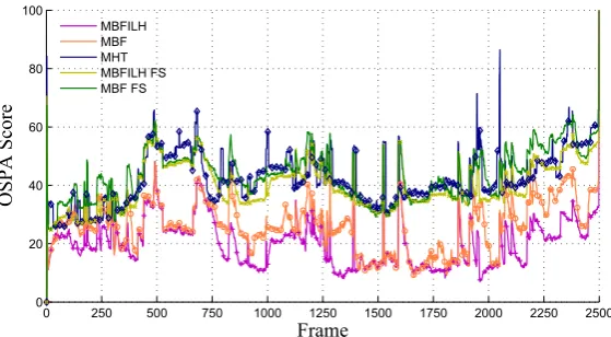
Figure 5. Average OSPA scores for all filter configurations over2500frames in the 2003 PETS INMOVE dataset. A lower score corresponds to better performance as the OSPA metric measures the distance between estimated target tracks and ground truth.
Table 1. Mean OSPA scores of the average Monte-Carlo trials for all filter configurations in the 2003 PETS INMOVE dataset. Best score(s) emphasized in bold.
Method Mean OSPA Scores
MHT 42.30
MBF FS 43.57
MBFILH FS 40.02
MBF 26.29
MBFILH 20.39
and p determines how harshly outliers (tracks which are farther away than the cutoff) are penalized. As p
FNR TPR FPR MOTP MOTA 0
0.2 0.4 0.6 0.8 1
MOT Score
MHT MBF FS
MBFILH FS
(a)
FNR TPR FPR MOTP MOTA
0 0.2 0.4 0.6 0.8 1
MOT Score
MBF
MBFILH
(b)
Figure 6. CLEAR MOT metric scores in the PETS dataset for a) the MBF FS and MBFILH FS in the PETS dataset and b) the MBF and MBFILH.
We evaluate the same20previously discussed Monte-Carlo trials from the PETS dataset using the CLEAR MOT metric.4 For details on the CLEAR MOT metric, see [70]. We used a distance threshold (ratio of intersection to union of the area of the target’s bounding box to the area of the ground truth bounding box) of0.1. This threshold is restricted to values between0and1and is used to determine when a correspondence can no longer be made between the estimate and the ground truth and the error is then labeled a missed detection. The CLEAR MOT metric is comprised of the following components (↑↓indicate when better performance is represented by higher and lower values respectively):
1. FNR: false negative rate (↓). 2. TPR: true positive rate (↑). 3. FPR: false positive rate (↓). 4. TP: number of true positives (↑). 5. FN: number of false negatives (↓). 6. FP: number of false positives (↓). 7. IDSW: number of label/i.d. switches (↓). 8. MOTP: multi-object tracking precision (↑). 9. MOTA: multi-object tracking accuracy (↑).
Results for the the20Monte-Carlo trials for each filter configuration are summarized in Table 3. The FNR, TPR, FPR, MOTP and MOTA scores are shown in Fig. 6aand Fig. 6balong with the corresponding standard deviations to illustrate the variability in the trials.
The largest improvement observed from the addition of the ILH was in the IDSW and MOTA metrics. Over the20trials and2500image frames, the MBFILH FS achieves32(approximately 49%) fewer identity switches than the MBF FS and71 (approximately68%) fewer than the MHT. In addition, the MBFILH FS yields an MOTA score of86.2%, while the MBF FS and MHT MOTA scores are79.4%and77.8%, respectively. Superior performance is again seen in the MBF and MBFILH configurations. The effect of the ILH is even more pronounced in comparing the MBF and MBFILH. The MBFILH reduces the number of identity switches seen in the MBF by approximately68%and increases the MOTA score from81.8%to89.3%. Because these two metric scores are directly influenced by labeling/i.d. error, the observed increases in these performance metrics suggest that the ILH term is able to significantly reduce the need for data association.
Figure 7.Illustrative scenarios in which the OSPA scores of the trackers under consideration differ significantly as visible in Fig. 5. The top row shows MHT results, middle row shows MBF results, and the bottom row shows MBFILH results all in the low resolution 2003 PETS INMOVE dataset. The numbers in green in the top row correspond to the object identifiers for the MHT. The numbers in black above the targets in the second and third rows correspond to the target identifier as well as the MBF estimate confidence level. In frames980,
FNR TPR FPR MOTP MOTA 0
0.1 0.2 0.3 0.4 0.5 0.6 0.7 0.8 0.9 1
MOT Score
MBF MBFILH
Figure 8.CLEAR MOT metric scores for the MBF and MBFILH in the reduced resolution AFL dataset.
Table 2.Summary of full resolution AFL CLEAR MOT metric scores. Best score(s) emphasized in bold.
Method MOTP MOTA
SMOT [71] 60.8% 16.7%
DCO [72] 63.3% 29.7%
[67] (no init) 64.1% 32.0%
[67] (no LDA) 63.6% 39.0%
[67] (full) 63.6% 41.4%
MBFILH 52.8% 66.3%
5.2. Australian Rules Football League
The second dataset we considered was the AFL dataset presented by Milanet al. in [67]. This dataset consists of299frames of an Australian Rules Football league match. Milanet al. explain that the AFL dataset is especially challenging for two reasons: 1) there is regular and frequent crowding of targets, and 2) contact and overlap among targets is common. We evaluate the ILH in this dataset using both reduced resolution images (320×240), and for direct comparison to results presented in [67], full resolution images (842×638).
We trained the MBF and MBFILH configurations to track all players and performed15 Monte-Carlo trials with320×240resolution. We then performed another20Monte-Carlo trials with842×638resolution evaluating only the MBFILH.
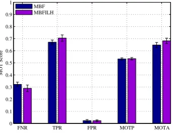
The CLEAR MOT metrics were used to evaluate the performance of each configuration in the reduced and full resolution trials. Again, a distance threshold of0.1was used. FNR, TPR, FPR, MOTP, and MOTA scores, along with standard deviations, are shown for the reduced resolution trials in Fig.8. Full resolution results are compared in Table2to results presented in [67].
As to be expected, results are generally lower (for both reduced and full resolution trials) in this more challenging dataset than they were in the 2003 PETS INMOVE dataset. Despite overall lower scores, in the reduced resolution trials, the ILH term still reduced the number of identity switches of the MBF, on average, by 4(approximately22%) and increased the MOTA score from64.8%to68.2%.
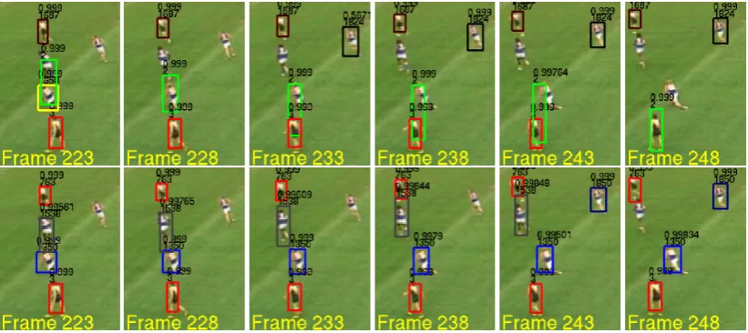
Some qualitative results from the reduced resolution trials are shown in Fig. 9. The sequence of images consists of five targets interacting in close proximity, presenting a difficult tracking scenario for any multi-target tracker. The performance of the MBF and MBFILH are qualitatively compared. While both configurations fail to correctly track all five targets, the MBFILH is better able to track more of the targets in extremely close proximity. See the caption of Fig.9for a more detailed explanation.
Figure 9.This is a particularly challenging sequence of low resolution AFL image frames (223-248). There are numerous overlapping and interacting targets. The top row are MBF results and the bottom row are MBFILH results. Note that in frame223, the MBF drops a target (the one with the yellow bounding box) while the MBFILH does not. Also, in frames233-243, the MBF target with the green bounding box starts to drift towards the target with the red bounding box, before finally merging in frame248, while the MBFILH is able to track these targets without drifting or falsely merging targets. However, the MBFILH does take longer to track the target farthest to the right in the images.
histograms, and the players’ torsos have the highest contrast with the background, the MBF is essentially only tracking the upper half of the players). In attempt to remedy this effect, the size estimates of the MBFILH in full resolution images were adjusted with a constant offset, however, this did not entirely eliminate the problem and explains the relatively poor performance of the MBFILH with respect to the MOTP metric in the full resolution trials (52.8%compared to the best result of64.1%).
Despite the unimpressive MOTP scores, the MBFILH scores extremely well in the full resolution dataset with respect to the MOTA metric. As illustrated in Table2, the MBFILH achieves an MOTA score of66.3% and the next highest performing method achieves41.4%.
5.3. TUD-Stadtmitte
We evaluate the performance of the ILH in a much different situation than the previously examined ‘sport player tracking’ type of scenarios. For this we use the TUD-Stadtmitte [68] dataset, which consists of 179 images of real data as pedestrians navigate through a street. This dataset is challenging because there are severe and frequent occlusions and the position of the camera allows for a wide range of target sizes (some targets are farther away and appear much smaller than targets that are closer), which illustrates another advantage of our approach: the ability to adapt to different target sizes online. We use full resolution images (640×480) for this evaluation. In order to track pedestrians in this dataset, we use the much more general pedestrian detector-based likelihood function in Eq. (10) with the multi-Bernoulli filter without the ILH (MBF PD) and with the ILH (MBFILH PD).
We carried out10Monte-Carlo trials for each filter configuration (MBF PD and MBFILH PD) and used the evaluation code made publicly available by Milanet al. in [53]5to compute the evaluation metrics. The different measures calculated in this evaluation are:
1. Rcll: recall - the percentage of detected targets (↑).
2. Prcn: precision - the percentage of correctly detected targets (↑). 3. FAR: number of false alarms per frame (↓).
Table 3.Summary of 2003 PETS INMOVE CLEAR MOT metric scores. Best score(s) emphasized in bold.
Method FNR TPR FPR TP FN FP IDSW MOTP MOTA
MHT 13.3% 86.0% 8.2% 14789 2293 1415 104 20.9% 77.8%
MBF FS 17.4% 82.1% 2.7% 14117 3004 465 65 24.4% 79.4%
MBFILH FS 10.7% 89.1% 2.9% 15308 1846 496 33 24.0% 86.2%
MBF 16.3% 83.3% 1.5% 14322 2803 264 62 45.1% 81.8%
MBFILH 9.2% 90.7% 1.4% 15583 1585 234 20 45.7% 89.3%
Table 4.Mean metric scores for10trials of the MBF PD and MBFILH PD in the TUD-Stadtmitte dataset. Best score(s) emphasized in bold where applicable.
Method Rcll Prcn FAR MT PT ML FP FN IDs FM MOTA MOTP MOTAL
MBF PD 58.54% 88.00% 0.52 3.10 6.70 0.20 92.7 479.30 8.8 12.10 49.76% 66.53% 50.43% MBFILH PD 60.91% 90.79% 0.40 3.70 6.10 0.20 71.50 451.90 5.70 12.90 54.23% 65.44% 54.65%
4. GT: number of ground truth trajectories. 5. MT: number of mostly tracked trajectories (↑). 6. PT: number of partially tracked trajectories. 7. ML: number of mostly lost trajectories (↓). 8. FP: number of false positives (↓).
9. FN: number of false negatives (↓). 10. IDs: number of i.d. switches (↓). 11. FM: number of fragmentations (↓).
12. MOTA: multi-object tracking accuracy in [0,100] (↑). 13. MOTP: multi-object tracking precision in [0,100] (↑).
14. MOTAL: multi-object tracking accuracy in [0,100] with log10(IDs) (↑).
Full results are presented in Table4and a selected number of CLEAR MOT metrics are shown in Fig.10. The ILH term improved the MOTA score of the MBF PD from 49.76% to54.23%. In addition, the average number of i.d. switches dropped from8.8to5.7(approximately35%reduction). In fact all scores were improved except for the ML metrics, which remained the same for both MBF PD and MBFILH PD, and the MOTP, which was slightly lower for the MBFILH PD (65.44%) than the MBF PD (66.53%). The reason for this slight decrease in MOTP performance is probably due to the ILH term forcing targets apart when they are extremely close. While this prevents unnecessary merging and i.d. switching, it may also cause estimates to be slightly shifted from the actual target. However, this is a relatively small decrease in MOTP performance, especially in comparison to the increases achieved in the MOTA, IDs, and other metrics. Figure11shows some snapshots of the results on the TUD-Stadtmitte dataset.
6. Conclusion
In this paper, an interactive likelihood for the multi-Bernoulli filter was introduced. The interactive likelihood is a simple, yet effective way for reducing the need for data association. This is done by making the particle likelihood proportional to its distance (in pixels) to all other particles for all other existing targets. This allows for greater particle and target interaction. The most important feature of the proposed interactive likelihood is that it is constructed entirely within the RFS-Bayesian framework, and therefore eliminates the need for heuristic ad-hoc data association approaches.
Recall Precision MOTA MOTP MOTAL 0
20 40 60 80 100
Metric Scores
MBF MBFILH
Figure 10.CLEAR MOT metric scores for the MBFILH PD in the TUD-Stadtmitte dataset.
INMOVE, AFL, and TUD-Stadtmitte) and well known metrics (OSPA and CLEAR MOT) in order to evaluate the performance of the various different filter configurations. Results indicate that the interactive likelihood term reduces the need for data association and increases the overall tracking performance of the multi-Bernoulli filter. Specifically, in all three datasets, the state-of-the-art RFS-based multi-Bernoulli filter saw accuracy improvements with the addition of the ILH term. The addition of the pedestrian detector makes the approach much more general, allowing the multi-Bernoulli filter to perform well in ‘real tracking’ situations, such as that depicted in the TUD-Stadtmitte dataset.
Despite the observed improvements, there are some limitations to this approach. The most relevant of which is computation time. Even though, for a bounded number of particles, the computation time isO(n2), wherenis the number of targets, in practice a significant amount of time is spent calculating all the distances between all particles. Therefore, plans for the immediate future are to investigate ways for increasing the overall speed of the algorithm. For example, due to their nature, the calculations are highly parallelizable and lend themselves to GPU implementations. Another potential way to achieve speed increases is to use more efficient algorithms for particle computation, such as quadtrees [73]. It should be noted, however, that distance computation is not the main bottleneck of the tracking algorithm as a whole. Sampling the image patches and computing their likelihoods is what dominates the computation time.
As mentioned in Section4, the parameters of the interactive likelihood σ and ζ and of the pedestrian detector γ were all determined empirically. More sophisticated and rigorous search methods could be employed or approaches to automatically learn these parameters based on characteristics of the datasets could be developed. In particular, prior distributions parameterized by characteristics of the dataset (such as the video resolution) could be employed to estimate these parameters within a Bayesian framework. This would almost certainly result in improved performance.
Another limitation is that the RFS-based tracking methods require birth and death models. These models are often application specific and therefore must be changed or modified based on the application, which is cumbersome for obvious reasons. Hence, in order to make this approach much more general, situation independent birth and death models are necessary. This would also allow for a much closer comparison to the most current benchmarks [53] and [54]. Measurement-driven birth models, as proposed initially in [74] and later extended to the Multi-Bernoulli filter for radar tracking applications in [75], provide a promising framework to address this problem.
Finally, our proposed approach does not take into consideration the extended target scenario in which a single target may generate multiple distinct measurements. Hence, scenarios involving, for example, extended concave targets [76] might still cause confusion. Although ad-hoc solutions that take into consideration the expected size and concavity of the targets could be employed to overcome this limitation, a more principled solution would be to utilize RFS-based extended target tracking approaches such as proposed in [77] while taking into account the expected distribution of the extended targets in the computation of the ILH.
Acknowledgments: The authors would like to thank Reza Hoseinnezhad for kindly sharing his implementation of the multi-Bernoulli filter.
Author Contributions: Anthony Hoak and Henry Medeiros conceived and designed the algorithm and the experiments. Anthony Hoak was responsible for most of the implementation of the algorithms. Richard J. Povinelli provided suggestions in the proposed method and its evaluation and assisted in the preparation of the manuscript.
Conflicts of Interest:The authors declare no conflict of interest.
References
1. Mallick, M.; Vo, B.N.; Kirubarajan, T.; Arulampalam, S. Introduction to the issue on multitarget tracking. Selected Topics in Signal Processing, IEEE Journal of2013,7, 373–375.
2. Stone, L.D.; Streit, R.L.; Corwin, T.L.; Bell, K.L.Bayesian multiple target tracking; Artech House, 2013.
3. Milan, A.; Leal-Taixé, L.; Schindler, K.; Reid, I. Joint tracking and segmentation of multiple targets. Proceedings of the IEEE Conference on Computer Vision and Pattern Recognition, 2015, pp. 5397–5406.
5. Hwang, I.; Balakrishnan, H.; Roy, K.; Tomlin, C. Multiple-target tracking and identity management in clutter, with application to aircraft tracking. American Control Conference, 2004. Proceedings of the 2004, 2004, Vol. 4, pp. 3422–3428 vol.4.
6. Bar-Shalom, Y. Multitarget-multisensor tracking: Applications and advances. Volume III. Norwood, MA, Artech House, Inc., 20002000.
7. Bobinchak, J.; Hewer, G. Apparatus and method for cooperative multi target tracking and interception, 2008. US Patent 7,422,175.
8. Soto, C.; Song, B.; Roy-Chowdhury, A.K. Distributed multi-target tracking in a self-configuring camera network. Computer Vision and Pattern Recognition, 2009. CVPR 2009. IEEE Conference on, 2009, pp. 1486–1493.
9. Wang, X. Intelligent multi-camera video surveillance: A review. Pattern Recognition Letters2013,34, 3. Extracting Semantics from Multi-Spectrum Video.
10. Kamath, S.; Meisner, E.; Isler, V. Triangulation Based Multi Target Tracking with Mobile Sensor Networks. Proceedings 2007 IEEE International Conference on Robotics and Automation, 2007, pp. 3283–3288.
11. Coue, C.; Fraichard, T.; Bessiere, P.; Mazer, E. Using Bayesian Programming for multi-sensor multi-target tracking in automotive applications. Robotics and Automation, 2003. Proceedings. ICRA ’03. IEEE International Conference on, 2003, Vol. 2, pp. 2104–2109 vol.2.
12. Ong, L.; Upcroft, B.; Bailey, T.; Ridley, M.; Sukkarieh, S.; Durrant-Whyte, H. A decentralised particle filtering algorithm for multi-target tracking across multiple flight vehicles. 2006 IEEE/RSJ International Conference on Intelligent Robots and Systems, 2006, pp. 4539–4544.
13. Premebida, C.; Nunes, U. A Multi-Target Tracking and GMM-Classifier for Intelligent Vehicles. 2006 IEEE Intelligent Transportation Systems Conference, 2006, pp. 313–318.
14. Jia, Z.; Balasuriya, A.; Challa, S. Recent Developments in Vision Based Target Tracking for Autonomous Vehicles Navigation. 2006 IEEE Intelligent Transportation Systems Conference, 2006, pp. 765–770.
15. Choi, J.; Ulbrich, S.; Lichte, B.; Maurer, M. Multi-Target Tracking using a 3D-Lidar sensor for autonomous vehicles. 16th International IEEE Conference on Intelligent Transportation Systems (ITSC 2013), 2013, pp. 881–886. 16. Ristic, B.; Vo, B.N.; Clark, D.; Vo, B.T. A Metric for Performance Evaluation of Multi-Target Tracking Algorithms.
Signal Processing, IEEE Transactions on2011,59, 3452–3457.
17. Reuter, S.; Vo, B.T.; Vo, B.N.; Dietmayer, K. Multi-object tracking using labeled multi-Bernoulli random finite sets. Information Fusion (FUSION), 2014 17th International Conference on, 2014, pp. 1–8.
18. Vo, B.T.; Vo, B.N. Labeled Random Finite Sets and Multi-Object Conjugate Priors. IEEE Transactions on Signal Processing2013,61, 3460–3475.
19. Reuter, S.; Vo, B.T.; Vo, B.N.; Dietmayer, K. The Labeled Multi-Bernoulli Filter. IEEE Transactions on Signal Processing2014,62, 3246–3260.
20. Vo, B.N.; Vo, B.T.; Phung, D. Labeled Random Finite Sets and the Bayes Multi-Target Tracking Filter. IEEE Transactions on Signal Processing2014,62, 6554–6567.
21. Papi, F.; Vo, B.N.; Vo, B.T.; Fantacci, C.; Beard, M. Generalized Labeled Multi-Bernoulli Approximation of Multi-Object Densities. IEEE Transactions on Signal Processing2015,63, 5487–5497.
22. Vo, B.N.; Vo, B.T.; Hoang, H.G. An Efficient Implementation of the Generalized Labeled Multi-Bernoulli Filter. IEEE Transactions on Signal Processing2017,65, 1975–1987.
23. Ouyang, W.; Wang, X. Joint deep learning for pedestrian detection. Computer Vision (ICCV), 2013 IEEE International Conference on. IEEE, 2013, pp. 2056–2063.
24. Fortmann, T.E.; Bar-Shalom, Y.; Scheffe, M. Multi-target tracking using joint probabilistic data association. Decision and Control including the Symposium on Adaptive Processes, 1980 19th IEEE Conference on, 1980, pp. 807–812. 25. Hoseinnezhad, R.; Vo, B.N.; Vo, B.T.; Suter, D. Visual tracking of numerous targets via multi-Bernoulli filtering of
image data. Pattern Recognition2012,45, 3625–3635.
26. Ristic, B.; Vo, B.T.; Vo, B.N.; Farina, A. A Tutorial on Bernoulli Filters: Theory, Implementation and Applications. Signal Processing, IEEE Transactions on2013,61, 3406–3430.
27. Vo, B.N.; Vo, B.T.; Pham, N.T.; Suter, D. Joint Detection and Estimation of Multiple Objects From Image Observations. Signal Processing, IEEE Transactions on2010,58, 5129–5141.
29. Vo, B.T.; Vo, B.N. A random finite set conjugate prior and application to multi-target tracking. Intelligent Sensors, Sensor Networks and Information Processing (ISSNIP), 2011 Seventh International Conference on, 2011, pp. 431–436.
30. Hoseinnezhad, R.; Vo, B.N.; Vo, B.T. Visual Tracking in Background Subtracted Image Sequences via Multi-Bernoulli Filtering.Signal Processing, IEEE Transactions on2013,61, 392–397.
31. Hoseinnezhad, R.; Vo, B.N.; Suter, D.; Vo, B.T. Multi-object filtering from image sequence without detection. Acoustics Speech and Signal Processing (ICASSP), 2010 IEEE International Conference on, 2010, pp. 1154–1157. 32. Maggio, E.; Taj, M.; Cavallaro, A. Efficient Multitarget Visual Tracking Using Random Finite Sets. IEEE
Transactions on Circuits and Systems for Video Technology2008,18, 1016–1027.
33. Rezatofighi, S.H.; Milan, A.; Zhang, Z.; Shi, Q.; Dick, A.; Reid, I. Joint probabilistic data association revisited. Proceedings of the IEEE International Conference on Computer Vision, 2015, pp. 3047–3055.
34. Lee, H.; Grosse, R.; Ranganath, R.; Ng, A.Y. Convolutional deep belief networks for scalable unsupervised learning of hierarchical representations. Proceedings of the 26th Annual International Conference on Machine Learning. ACM, 2009, pp. 609–616.
35. Hinton, G.E.; Osindero, S.; Teh, Y.W. A fast learning algorithm for deep belief nets. Neural computation2006, 18, 1527–1554.
36. Krizhevsky, A.; Sutskever, I.; Hinton, G.E. Imagenet classification with deep convolutional neural networks. Advances in neural information processing systems, 2012, pp. 1097–1105.
37. Sermanet, P.; Kavukcuoglu, K.; Chintala, S.; LeCun, Y. Pedestrian detection with unsupervised multi-stage feature learning. Proceedings of the IEEE Conference on Computer Vision and Pattern Recognition, 2013, pp. 3626–3633. 38. Ouyang, W.; Wang, X. A discriminative deep model for pedestrian detection with occlusion handling. Computer
Vision and Pattern Recognition (CVPR), 2012 IEEE Conference on, 2012, pp. 3258–3265.
39. Ouyang, W.; Zeng, X.; Wang, X. Modeling mutual visibility relationship in pedestrian detection. Proceedings of the IEEE Conference on Computer Vision and Pattern Recognition, 2013, pp. 3222–3229.
40. Zeng, X.; Ouyang, W.; Wang, X. Multi-stage contextual deep learning for pedestrian detection. Proceedings of the IEEE International Conference on Computer Vision, 2013, pp. 121–128.
41. Luo, P.; Tian, Y.; Wang, X.; Tang, X. Switchable deep network for pedestrian detection. Proceedings of the IEEE Conference on Computer Vision and Pattern Recognition, 2014, pp. 899–906.
42. Milan, A.; Rezatofighi, S.H.; Dick, A.R.; Schindler, K.; Reid, I.D. Online Multi-target Tracking using Recurrent Neural Networks. CoRR2016,abs/1604.03635.
43. Chen, X.; Qin, Z.; An, L.; Bhanu, B. An Online Learned Elementary Grouping Model for Multi-target Tracking. The IEEE Conference on Computer Vision and Pattern Recognition (CVPR), 2014.
44. Tang, S.; Andres, B.; Andriluka, M.; Schiele, B. Subgraph Decomposition for Multi-Target Tracking. The IEEE Conference on Computer Vision and Pattern Recognition (CVPR), 2015.
45. Shafique, K.; Shah, M. A noniterative greedy algorithm for multiframe point correspondence. Pattern Analysis and Machine Intelligence, IEEE Transactions on2005,27, 51–65.
46. Bar-Shalom, Y.; Daum, F.; Huang, J. The probabilistic data association filter.Control Systems, IEEE2009,29, 82–100. 47. Oh, S.; Russell, S.; Sastry, S. Markov Chain Monte Carlo Data Association for Multi-Target Tracking. IEEE
Transactions on Automatic Control2009,54, 481–497.
48. Choi, W. Near-Online Multi-target Tracking with Aggregated Local Flow Descriptor. Proceedings of the IEEE International Conference on Computer Vision, 2015, pp. 3029–3037.
49. Wang, B.; Wang, G.; Chan, K.L.; Wang, L. Tracklet Association by Online Target-Specific Metric Learning and Coherent Dynamics Estimation. arXiv preprint arXiv:1511.066542015.
50. Bewley, A.; Ge, Z.; Ott, L.; Ramos, F.; Upcroft, B. Simple Online and Realtime Tracking. arXiv preprint arXiv:1602.007632016.
51. Kim, C.; Li, F.; Ciptadi, A.; Rehg, J.M. Multiple Hypothesis Tracking Revisited. Proceedings of the IEEE International Conference on Computer Vision, 2015, pp. 4696–4704.
52. Milan, A.; Schindler, K.; Roth, S. Multi-Target Tracking by Discrete-Continuous Energy Minimization. IEEE Transactions on Pattern Analysis and Machine Intelligence2016,38, 2054–2068.
53. Leal-Taixé, L.; Milan, A.; Reid, I.; Roth, S.; Schindler, K. MOTchallenge 2015: Towards a benchmark for multi-target tracking. arXiv preprint arXiv:1504.019422015.
55. Dehghan, A.; Tian, Y.; Torr, P.H.S.; Shah, M. Target Identity-aware Network Flow for online multiple target tracking. 2015 IEEE Conference on Computer Vision and Pattern Recognition (CVPR), 2015, pp. 1146–1154.
56. Porikli, F. Needle picking: a sampling based Track-before-detection method for small targets. In SPIE Defense, Security, and Sensing; for Optics, I.S.; Photonics.., Eds., 2010, pp. 769803–769803.
57. Davey, S.; Rutten, M.; Cheung, B. A comparison of detection performance for several track-before-detect algorithms. EURASIP Journal on Advances in Signal Processing2008.
58. Mahler, R.P.Statistical multisource-multitarget information fusion; Artech House, Inc, 2007. 59. Mahler, R.Random set theory for target tracking and identification; CRC press Boca Raton, 2001.
60. Mahler, R.P.S. “Statistics 101" for multisensor, multitarget data fusion.Aerospace and Electronic Systems Magazine, IEEE2004,19, 53–64.
61. Vo, B.N.; Singh, S.; Doucet, A. Sequential Monte Carlo methods for multitarget filtering with random finite sets. Aerospace and Electronic Systems, IEEE Transactions on2005,41, 1224–1245.
62. Qu, W.; Schonfeld, D.; Mohamed, M. Real-Time Distributed Multi-Object Tracking Using Multiple Interactive Trackers and a Magnetic-Inertia Potential Model. Multimedia, IEEE Transactions on2007,9, 511–519.
63. Xiao, J.; Oussalah, M. Collaborative Tracking for Multiple Objects in the Presence of Inter-Occlusions. IEEE Transactions on Circuits and Systems for Video Technology2016,26, 304–318.
64. Yang, B.; Yang, R. Interactive particle filter with occlusion handling for multi-target tracking. 2015 12th International Conference on Fuzzy Systems and Knowledge Discovery (FSKD), 2015, pp. 1945–1949.
65. Dollar, P.; Wojek, C.; Schiele, B.; Perona, P. Pedestrian detection: A benchmark. Computer Vision and Pattern Recognition, 2009. CVPR 2009. IEEE Conference on, 2009, pp. 304–311. ID: 1.
66. Antunes, D.M.; de Matos, D.M.; Gaspar, J. A Library for Implementing the Multiple Hypothesis Tracking Algorithm. arXiv preprint arXiv:1106.22632011.
67. Milan, A.; Gade, R.; Dick, A.; Moeslund, T.B.; Reid, I. Improving Global Multi-target Tracking with Local Updates. Workshop on Visual Surveillance and Re-Identification, 2014.
68. Andriluka, M.; Roth, S.; Schiele, B. Monocular 3D pose estimation and tracking by detection. Computer Vision and Pattern Recognition (CVPR), 2010 IEEE Conference on. IEEE, 2010, pp. 623–630.
69. Schuhmacher, D.; Vo, B.T.; Vo, B.N. A Consistent Metric for Performance Evaluation of Multi-Object Filters. Signal Processing, IEEE Transactions on2008,56, 3447–3457.
70. Bernardin, K.; Stiefelhagen, R. Evaluating multiple object tracking performance: the CLEAR MOT metrics. Journal on Image and Video Processing2008,2008, 1.
71. Dicle, C.; Camps, O.; Sznaier, M. The way they move: Tracking multiple targets with similar appearance. Proceedings of the IEEE International Conference on Computer Vision, 2013, pp. 2304–2311.
72. Milan, A.; Schindler, K.; Roth, S. Detection- and Trajectory-Level Exclusion in Multiple Object Tracking. Computer Vision and Pattern Recognition (CVPR), 2013 IEEE Conference on, 2013, pp. 3682–3689.
73. Park, J.; Tabb, A.; Kak, A.C. Hierarchical Data Structure for Real-Time Background Subtraction. Image Processing, 2006 IEEE International Conference on, 2006, pp. 1849–1852.
74. Ristic, B.; Clark, D.; Vo, B.N.; Vo, B.T. Adaptive Target Birth Intensity for PHD and CPHD Filters.IEEE Transactions on Aerospace and Electronic Systems2012,48, 1656–1668.
75. Yuan, C.; Wang, J.; Lei, P.; Bi, Y.; Sun, Z. Multi-Target Tracking Based on Multi-Bernoulli Filter with Amplitude for Unknown Clutter Rate. Sensors2015,15, 29804.
76. Zea, A.; Faion, F.; Baum, M.; Hanebeck, U.D. Level-Set Random Hypersurface Models for tracking non-convex extended objects. Proceedings of the 16th International Conference on Information Fusion, 2013, pp. 1760–1767. 77. Beard, M.; Reuter, S.; Granström, K.; Vo, B.T.; Vo, B.N.; Scheel, A. Multiple Extended Target Tracking With Labeled
Random Finite Sets. IEEE Transactions on Signal Processing2016,64, 1638–1653.
c