Article
1
Average Generalized Ambiguity Function Analysis
2
for Passive Bistatic SAR Systems Using PSK
3
Modulating Signal
4
Zhiping Yin 1, Lei Zhang 1, Jinbao Xie 1, Jun Yang 1, Guangsheng Deng 1 and Zhaoxian Zeng 2,*
5
1 Academy of Photoelectric Technology, Hefei University of Technology, Hefei 230009, China;
6
[email protected] (Z.Y.); [email protected] (L.Z.); [email protected] (J.X.);
7
[email protected] (J.Y.); [email protected] (G.D.)
8
2 Beijing System Engineering Institute, Beijing, China
9
* Correspondence: [email protected]
10
Abstract: The formula of the Generalized Ambiguity Function (GAF) of passive bistatic SAR
11
system using the non-cooperative illuminators which transmit PSK modulating signals is derived
12
to analyze the spatial resolution of the system. The average GAF is introduced to remove the effect
13
of particular sequence of symbols on resolution because the particular sequence of symbols is
14
usually unpredictable before being received. The influence of the waveform parameters of the PSK
15
modulating signals, such as length of the symbol sequence and roll-off factor, on spatial resolution
16
is investigated by numerical simulation. It is confirmed that the influence of the length of the
17
symbol sequence and roll-off factor is very slight but still exists.
18
Keywords: average generalized ambiguity function; passive bistatic SAR; PSK modulating signal;
19
spatial resolution
20
1. Introduction
21
In recent years, the passive bistatic SAR/ISAR systems, which use the non-cooperative
22
illuminators as the transmitters of opportunity, have drawn a lot of attention all over the world due
23
to their prominent advantages in comparison to active radars, such as low cost, low probability of
24
interception, flexible configuration, coverage characteristics and availability of rich illuminator
25
sources [1, 2]. The passive radar imaging systems utilize broadcasting station [3], television
26
transmitting tower [4], broadcasting satellite [5, 6], navigation satellite [7, 8], communication base
27
station [9] and wireless networks [10, 11] as their illuminators with a bistatic geometry
28
configuration. Phase shift keying (PSK) modulating signal is a potential source of illumination for
29
passive imaging system due to its wide application in communication, radar, navigation and so on.
30
The feasibility of two-dimensional imaging using scattered PSK-modulated communication signals
31
was investigated by numerical simulation [12]. The passive SAR system based on digital video
32
broadcasting satellites with QPSK modulation was studied using simulation [13] and experiment [14,
33
15], and its resolution capability was evaluated by the analysis of the wavenumber domain coverage
34
in [13]. The ISAR image of a vehicle was obtained by passive radar system using DVB-S signals
35
which implements QPSK modulation. In addition, PSK modulation techniques are widely used in
36
the satellite navigation systems and the feasibility of the passive bistatic SAR systems has been
37
theoretically and experimentally verified by using GPS [16], GLONASS [17, 18], GALILEO [7] and
38
BDS [19] signals.
39
The spatial resolution is one key factor of the performance for SAR/ISAR imaging system. In
40
traditional radar systems, the resolution which describes the capacity to separate two or more
41
targets can be usually analyzed by calculating the ambiguity function. For SAR/ISAR imaging
42
system, the generalized ambiguity function (GAF) was formed to evaluate the spatial resolution [20],
43
which has been used in several papers to discuss the passive system resolution. In [21], the GAF of
44
the bistatic SAR is deduced under narrowband assumption where the signal waveform was
45
approximated by a Gaussian or rectangle pulse functions, and then the theoretical GAF equation of
46
the bistatic SAR was verified by an experimental passive system consisting of GLONASS satellites as
47
transmitters and a fixed receiver [22]. In [23], the GAF of a multiple antennas multiple frequencies
48
radar system was introduced, which described the effect of the signal bandwidth without the signal
49
waveform on the resolution. Soon after this work, the experimental result of the GAF of multistatic
50
SAR was achieved by combining reflected signals from several GLONASS satellites [24].
51
The present studies mentioned above about GAF of the passive SAR/ISAR systems mainly
52
focused on the simplified signal model, and the effect of signal waveform on spatial resolution was
53
ignored. In consideration of ambiguity function theory that the modulation signal waveform will
54
impact on the system’s ability to discriminate different targets in the delay-Doppler domain, it’s very
55
important to investigate the effect of signal waveform on profile of GAF to evaluate the performance
56
of spatial resolution for the passive SAR/ISAR systems. Hence, this paper tries to study the GAF of
57
the passive SAR system based on PSK modulating signals.
58
In this work, we derive the theoretical formula of the GAF of passive bistatic SAR system using
59
the non-cooperative illuminators which transmit PSK modulating signal. The concept of average
60
ambiguity function is introduced in order to analyze the resolution capability of the passive bistatic
61
SAR system independently of the particular sequence of symbols of the transmitted signal, because
62
the particular sequence of symbols is usually unpredictable before being received for passive
63
system. Then, the influence of the waveform parameters of the PSK modulating signals, such as
64
length of the symbol sequence and roll-off factor, on spatial resolution is discussed, while that of the
65
code width, the main factor in determining the resolution which has discussed in [21], is ignored in
66
this paper.
67
This paper is organized as follows. In Section 2 the geometry of the BISAR system is described
68
and the transmitted signal model for the passive radar system is presented. In Section 3 we define
69
and derive the average GAF of the BISAR system based on PSK modulating signals. In Section 4 the
70
simulated analysis is presented in order to demonstrate the resolution capability of the system.
71
Finally, concluding remarks are drawn in Section 5.
72
2. System and Signal
73
2.1 BISAR System Geometry
74
x
y
AB(x, y,z)
v
(x ,y ,z)
T T TT W
r
z
75
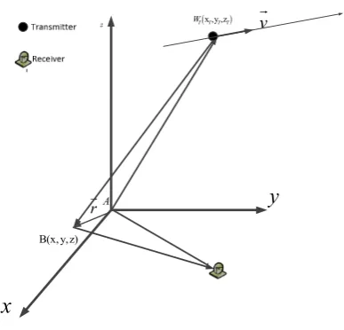
Figure 1. The BISAR geometry with a fixed receiver
76
Figure 1 shows a generalized geometry of a passive BISAR system. This configuration consists
77
of a stationary target with the invariable scattering coefficient, a moving transmitter of opportunity,
78
and a stationary receiver fixed on the ground. In this case, the distance between the transmitter and
79
the target point is much greater than the distance between the receiver and the target point. In order
80
to simplify the analysis, the three-dimensional coordinate system with the center of the target as
81
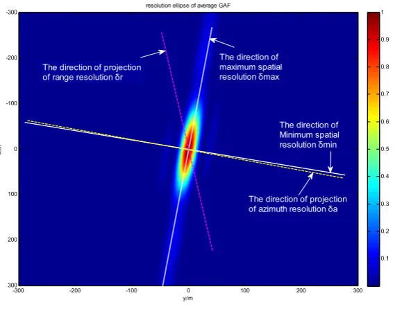
origin is established. Vectors and denote the position coordinate of the transmitter and the
receiver respectively. Vector is the velocity of the transmitter whose motion trajectory is a straight
83
line during integration time.
84
There are two time variables that need considering in the BISAR system. One variable t is the
85
fast time, which describes the propagation of the ranging waveform. The other variable is the slow
86
time u that specifies the position of the receiver and the transmitter. In the system shown in Figure 1,
87
only the position of the transmitter varies with the slow time u and the motion is much slower than
88
the propagation of the electromagnetic wave. Thus is a function about u and , and is
89
represented at slow time u as
90
0
( )
( )
T T
W u
=
W u
+ ⋅
v u
, (1)where ( ) is the position of the transmitter at the slow time instant u = u0.
91
2.2 Signal Model
92
Assuming that the envelope and the carrier of the transmitted signal are ( ) and
93
respectively, the echo signal of the point target A received by the receiver antenna can be
94
represented as
95
2 2 (t )
( , )
(
)e
j fc A j fdA AA A
s t u
=
σ
s t
−
τ
− π τe
− π −τ, (2)
In this equation, σ is the scattering coefficient of the target A, which is assumed to be constant
96
and independent of the distance from the transmitter to the target. Furthermore, and are the
97
time delay and the Doppler frequency respectively, which are the functions of slow time u. The
98
equations about and are defined as
99
( ) ( )
( ) ( )
( )
R T A c T
A d
T
A W A W u f A W u
f v
c c A W u
u
u
τ
= − + − = ⋅ −−
, (3)The PSK modulating signal transmitted by the illuminators of opportunity is pulse compression
100
signal and is usually applied in the SAR systems in order to acquire the low probability of intercept.
101
The expression of the unit energy complex envelope is defined as
102
-1 n 1 =0
1
( ) =
( -
)
N n
s t
c u t nT
N
, (4)where is the modulation code, which is usually pseudo-random or unpredictable, for the
103
illuminator of opportunity and N is the number of symbols. The pulse ( ) is a rectangular pulse
104
and T is the width in the fast time domain. In order to reduce inter symbol interference, a delayed
105
RRC filter is usually employed in systems as the pulse shaping filter. The equation of ( ) is
106
represented as
107
1
2
1
1
4
sin( (1 )) cos( (1 )) ( )
4 [1 ( ) ]
1 4
( 0) (1 )
2 2
( ) [(1 ) sin( ) (1 ) cos( )]
4 2 4 4
t t t
T T T
u t
t t
T T
u t
T T u t
T
π α π
α α
π α
α α
π
α π π
α π α π α
− + +
=
−
= = − +
= ± = + + −
,
(5)
where α is the roll-off factor of the filter, which lies in the interval [0,1] for all transmitters. Denoting
108
the Fourier transform of the pulse ( ) as ( ), | ( )| can be defined as
2
1
2
1
1
1
( )
[1 cos(
(
))]
2
2
2
2
0
T
f
T
T
T
U f
f
f
T
T
T
other
α
π
α
α
α
α
−
≤
−
+
+
=
+
−
≤
≤
, (6)
Having presented the BISAR system geometry and the expression of the transmitted signals,
110
the research now moves on to the study of the generalized ambiguity function in the following
111
section.
112
3. Ambiguity Function of BISAR
113
The spatial resolution of the remote sensing system is one of the key parameters and is defined
114
as the capacity to separate two or more targets in spatial domain. The ambiguity function (AF) is
115
usually studied to obtain the resolution of the system, in terms of range and speed. In order to study
116
the spatial resolution in SAR, the definition of radar AF has been extended to GAF by Tao Zeng, et
117
al. [21] and the equation is represented as
118
*
( )
r
s t u s t u dtdu
A( , ) ( , )
Bχ
=
, (7)where ( , ) and ( , ) are the complex envelopes of reflected signals from two point target
119
located at the points A and B, whose scattering coefficients are assumed as unit radar cross section.
120
Point A is the desired point scatterer to be evaluated, and B is an arbitrary point scatterer in the
121
vicinity of A. is the distance vector from A to B.
122
Different from the active radar which usually transmits deterministic signals, most of the
123
received signals of passive radar are non-deterministic due to the non-cooperative of the
124
illuminators. In the case of PSK modulating signals, the non-deterministic means the sequence of
125
symbols is pseudo-random, such as the signals from navigation system, or unpredictable, such as
126
the signals from communication system. In order to remove the impact of the non-deterministic of
127
the sequence of symbols on the profile of GAF, the concept of the average ambiguity function is
128
introduced here. The average ambiguity function defined by Cooper is generalized to the average
129
GAF of the BISAR system, which is written as follow
130
{ }
2{
* 2}
( )
( )
A( , ) ( , )
BA r
=
E
χ
r
=
E
s t u s t u dtdu
, (8)By substituting the expressions of the echo signals, the GAF of the system is represented as
131
' '
' '
2 1 1 1 1
* * 2
0 0 0 0
2 ( ) 2 ( ) 2 ( )
* '
1 1
2 ( ) 2 ( ) 2 (
* '
1 1
( ) { }
( ) ( )
( ) ( )
B A B A
c B A d d d B d A
B A B A
c B A d d d B d
N N N N
n n k k
n n k k
j f j f f t j f f
A B
j f j f f t j f f
A B
A r E c c c c
N
u t nT u t nT e e e dtdu
u t kT u t k T e e e
π τ τ π π τ τ
π τ τ π π τ
σ
τ
τ
τ
τ
− − − − = = = =
− − − −
− − − −
=
× − − − −
× − − − −
(
)
*)
A dtdu
τ
, (9)
where and are the time delay of the echo signals for target point A and arbitrary point B
132
respectively, and the expectation ∙ is with respect to the transmitted modulation code . All the
133
transmitted pulses are independent and identically distributed across symbol indices, and ∙ can
134
be written as below.
' '
' '
* * ' ' '
1,
,
;
{
}
1
,
,
;
0
n n k k
n n k k
E c c c c
n k n
k n n
others
=
=
=
=
=
≠
, (10)
Substituting the equation (10) and deducing this function from time domain to frequency
136
domain in accordance with Fourier transform, the equation (9) can be converted into
137
(
)
* * * 42 ( ) 2 ( )
2 ( )
*
2 ( ) 2 ( )
2 ( )
4 1 1
2 0 0, 2 ( ( ) ( ) ( ) ( ) ( ) ( ) ( ) B A
c B A d B d A B A
B A
c B A d B d A B A B A B A d d B A d d B A d d
j f j f f
j f
j f j f f
j f
N N
n k k n
j f (k
-U f f f U f
U f f f U f
U f f f U f
A r
e e e dfdu
e e e dfdu
N e π τ τ π τ τ π τ τ π τ τ π τ τ π τ τ π τ τ
σ
σ
− − − − − − − − − − = = ≠ − + − + − + − + = × × +
(
*)
2 ( ) 2 ( )
)
*
2 ( ) 2 ( )
2 ( ( ) )
( ) ( )
B A
c B A d B d A
B A
c B A d B d A B A
B A
d d
j f j f f
n)T
j f j f f
j f k -n T
U f f f U f
e e dfdu
e e e dfdu
π τ τ π τ τ π τ τ π τ τ π τ τ − − − − − − − + − + ×
, (11)
where ( )is the Fourier transform of the pulse ( ). The delay difference between the received
138
signals reflected by point A and B is defined as
139
( )
( )
T R T R
B A
W u
r
W
r
W u
W
c
c
τ τ
−
=
− +
−
−
+
, (12)
As is shown in Figure 1, the transmitter is usually far away from the target region and | | is
140
much smaller than the distance from the transmitter to the target. Denoting the unit vector in the
141
direction of the receiver as ( ) = ( ) ( ), the distance between the target and the receiver
142
is presented as
143
( )
( )
A( )
T T T
W u
− =
r
W u
−
i
u r
⋅
, (13)Meanwhile, the receiver is not far away from the target region and − needs to be
144
calculated accurately. By considering the assumptions above, the delay difference − is shown
145
as146
( )
A R R T B AW
r
W
i
u r
c
c
τ
−
τ
= −
⋅
+
− −
, (14)
Assuming the integration time was (i.e. ∈ − /2, + /2 ) and denoting as the
147
value at the midpoint of , the equation (14) is approximated by its first-order Taylor expansion at
148
=149
0 0 0( )
(
( ))
(
)
A A R R T T B AW
r
W
i
u
r
r
d i
u
u u
c
c
c
du
τ τ
−
= −
⋅
+
− −
+
−
−
, (15)
Denoting and as the delay difference and the Doppler frequency when = , then
150
0 ( ) A R R T dW r W
i u r
c c
τ
= − ⋅ + − −
, 0 ( TA( ))d c
d i u
r f f c du − =
, (16)
Therefore, the equation (14) can be simplified into
0
1
(
)
B A d d
c
f u u
f
τ
−
τ
=
τ
+
⋅
−
, (17)Meanwhile, the same approximation approach is applied and the phase term − is
152
approximated. The result of the simplification is represented as
153
0
2 2
0 2
(
( ))
(
)
(
)
(
)
A
B A c c T
d B d A R R
R R
d
f v r
f v
i
u
f
f
W
r
W
c
c
v r W
r
W
f u u
c r
τ
−
τ
=
⋅
+
⋅ −
− −
⋅
− −
+
−
, (18)
Considering the assumptions mentioned above and the characteristics of the signal which is
154
narrowband, the equation (11) becomes
155
0 2
2
( )
2 (1 )( )
4
1 1
2 2
2 2 2 2 ( ( ) )
2 0 0, ( )
1
( ) ( )
( ) ( )
R R
d
d d
v r W r W
j f u u
c r
N N
j f j f k -n T
n k k n
d d
A r e du
U f e df U f e df
N
K
m f
p
π
π τ π τ
σ
τ
⋅ − −
− −
− −
+ = = ≠
=
× +
=
, (19)
where K is the coefficient which is irrelevant to f and u, ( ) is the integral of variable u and ( )
156
is the integral of variable f.
157
Equation (19) indicates that the average GAF of BISAR system using PSK modulating signal is
158
presented as the production of two functions, ( ) and ( ), which is the same with the results
159
in [21] . The azimuth resolution and its direction can be obtained from the function ( ), which is
160
mainly determined by motion of the transmitter and the integration time. Function ( ), which
161
contains the parameters of the PSK modulating signals including the code-width, the length of the
162
symbols and the pulse shaped by RRC filter but excepting the particular sequence of symbols whose
163
influence has been removed by the average processing for GAF, gives the radar spatial performance
164
in the range domain. In a bistatic SAR system, the range resolution is in the direction of the bisector
165
of the bistatic angle and the azimuth resolution’s direction is specified by the equivalent motion
166
direction. Generally, a more general resolution in any arbitrary direction of the X-Y plane is defined
167
to analyze resolution capability of the system for the earth observation, so the resolution ellipse
168
projected onto the X-Y plane is chosen in order to give tools to the radar system to evaluate the
169
resolution capability [23]. and are defined in the direction of the projection of range and
170
azimuth resolution onto the X-Y plane respectively. Figure 2 shows the projection of equation (19)
171
for a BISAR system using a GPS satellite that will be used in the simulation in the next section. On
172
the resolution ellipse, the maximum spatial resolution and minimum spatial resolution
173
are along the major axis and the minor axis respectively and are usually applied to characterize the
174
resolution capability. In this example, it can be clearly observed that the directions of projected
175
range resolution and projected azimuth resolution don’t overlap with that of the spatial
176
resolution is or respectively, but the direction of is very colse to that of .
177
Although the carrier frequency and signal bandwidth are the mainly decisive factors of the
178
profile of the average GAF of BISAR system using PSK modulating signal, the length of the symbols
179
and the pulse shaped by RRC filter may also have an impact on the average GAF of the system.
180
Hence, the average GAF of BISAR system is calculated and discussed in the following section to
181
evaluate the resolution performance of the system.
183
Figure 2. The resolution ellipse of the BISAR system and the directions of different resolution
184
4. Simulated Results and Analysis
185
In order to verify the average GAF of PSK modulation system mentioned in Section 3, the GAF
186
of a passive BISAR system consisting of a GPS satellite as illuminator of opportunity and a receiver
187
fixed on the ground is calculated by simulation. The GPS satellite runs over Hefei in one certain
188
moment, and its parameters are shown in Table 1 and Table 2. It is assumed that the motion of the
189
satellite is linear and the velocity is invariable during integration time. Meanwhile, the scattering
190
coefficients of all reflectors within the imaging area are equal to one and independent of the distance
191
from the transmitter to the target. Hence, an appropriate coordinate system is designed that X axis
192
and Y axis is coincident with the east and north respectively, Z axis passed through the Earth’s core,
193
and X-Y plane is tangent to the Earth’s surface. The target reflector to be analyzed is located at the
194
center of the X-Y plane and B is an arbitrary point in the X-Y plane.
195
Table. 1. The fundamental parameters of GPS satellite
196
Parameter Symbol Numerical Value
Carrier Frequency 1575.42MHz
Bandwidth of Signal B 1.023MHz
Width of Pulse T 1/1.023×10-6
Integration Time 60s
Velocity of Satellite (1.0962,-0.6366,-0.7552)×104
Initial Position of Satellite (447075.2875,
20227806.07,1618341.826)
Table. 2. The position of satellite as a function of integration time-- = 60
197
Satellite φe( )u0 θe( )u0 Δφe Δθe
SAT15 300° 78.5° 1.91° -0.167°
4.1 GAF VS Average GAF
198
The GAFs of the BISAR system using three kinds of pseudo-random symbols called M1, M2
199
and M3 with the number of the symbols of 1001 and the roll-off factor α of 0.22 are shown in Figure
200
3-5 respectively. The average GAF of the system with the same number of the symbols and roll-off
201
y/m
x/
m
resolution ellipse of average GAF
-300 -200 -100 0 100 200 300
-300
-200
-100
0
100
200
300
0.1 0.2 0.3 0.4 0.5 0.6 0.7 0.8 0.9 1
The direction of projection of range resolution δr
The direction of maximum spatial resolution δmax
The direction of projection of azimuth resolution δa
factor is also calculated and shown in Figure 6. In order to compare the resolution capability with
202
each other, the resolution slices along the major and minor axis are plotted in Figure 7 and Figure 8.
203
Figure 3. Generalized ambiguity function about M1 Figure 4. Generalized ambiguity function about M2
204
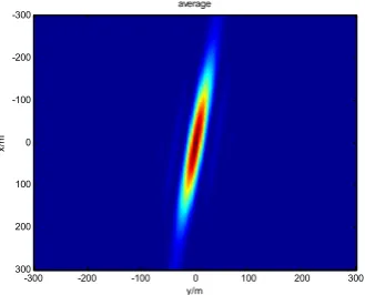
Figure 5. Generalized ambiguity function about M3 Figure 6. Average GAF of the BISAR system
205
Figure 7. The resolution slice along major axis Figure 8. The resolution slice along minor axis
As shown in Figure 3, 4 and 5, it can be observed that the system based on different sequences
206
with the same number of the symbols provides almost the same resolution ellipses, because these
207
sequences are only different in the transmitted symbol sequence. The resolution slices along the
208
major axis (Figure 7) demonstrate that their maximum spatial resolutions are exactly similar,
209
especially for the mainlobe. The resolution slices along the minor axis (Figure 8) are identical, for the
210
reason that the direction of and the direction of are basically consistent and the
211
transmitted waveform has little impact on the azimuth resolution. Hence, the difference among
212
their resolution ellipses caused by the different symbol sequence is very slight but still exists. Figure
213
6 shows the average GAF of the BISAR system. Comparing with Figure 3, 4 and 5, it is evident that
214
the average GAF suppresses the sidelobe resulted from the independence of the particular symbol
215
sequence. The independence of the particular symbol sequence means that the average GAF is more
216
useful for evaluating the resolution of passive BISAR system, especially for the system that use the
217
non-cooperative transmitters with unpredictable symbol sequences, such as PSK modulating
218
communication transmitters.
219
x/
m
y/m m1
-300 -200 -100 0 100 200 300
-300
-200
-100
0
100
200
300
x/
m
y/m m2
-300 -200 -100 0 100 200 300
-300
-200
-100
0
100
200
300
x/
m
y/m m3
-300 -200 -100 0 100 200 300
-300
-200
-100
0
100
200
300
x/m
y/m average
-300 -200 -100 0 100 200 300
-300
-200
-100
0
100
200
300
-10000 -800 -600 -400 -200 0 200 400 600 800 1000 0.1
0.2 0.3 0.4 0.5 0.6 0.7 0.8 0.9 1
distance/m
m1 m2 m3 average
-2000 -150 -100 -50 0 50 100 150 200 0.1
0.2 0.3 0.4 0.5 0.6 0.7 0.8 0.9 1
distance/m
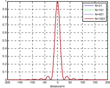
4.2 The Impact of Number of Symbols
220
It can be seen from the equation (19) that the number of symbols is one of the parameters for the
221
BISAR system using PSK modulation. In this part, four sequences of different lengths are chosen to
222
investigate the effect of length of the symbol sequence on the average GAFs. The roll-off factor is set
223
to 0.22 for all four sequences. The resolution slices along the major axis and minor axis are shown in
224
Figure 9 and Figure 10 respectively. It is obvious that the resolution slices along the major axis are
225
identical except for small difference in sidelobe and the lower sidelobe will be obtained when using
226
longer sequences. The resolution slices along the minor axis present the same curves which are
227
overlapping each other. So the maximum and minimum spatial resolutions of the BISAR system
228
based on four sequences of variable lengths are basically the same. The result indicates that the
229
number of symbols have little influence on the resolution ellipse of BISAR system.
230
Figure 9. Resolution slice of average GAFs based on the length of sequence along major axis
Figure 10. Resolution slice of average GAFs based on the length of sequence along minor axis
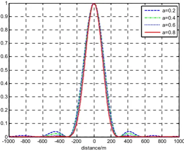
4.3 The Impact of Roll-off Factor
231
As mentioned above, the pulse waveform ( ) is obtained by applying a pulse shaping filter
232
to each pulse to reduce inter symbol interference. In this work, a delayed RRC filter is applied and
233
α=0.2, 0.4, 0.6, 0.8 are chosen as the roll-off factor to calculate the average GAF in order to analyze the
234
impact of the roll-off factor on the profile of average GAF. The resolution slices along the major axis
235
and minor axis are shown in Figure 11 and 12 respectively. It is obvious that the minimum spatial
236
resolutions are the same, and the maximum spatial resolutions present small difference
237
for different roll-off factors, which causes different resolution ellipses. Hence, it can be observed that
238
the BISAR system provides better resolution capability when the roll-off factor increases, because
239
the increase can make the bandwidth of the signal expand simultaneously. We plot the -3dB contour
240
of the spatial resolution along the major axis in Figure 13 to further study the effect of the roll-off
241
factor on the resolution ellipse. The results in Figure 13 indicate that the PSK modulating signal
242
whose roll-off factor is higher can have smaller maximum spatial resolution because of the tiny
243
change of bandwidth due to filtering. While the value of the roll-off factor increases from 0.2 to 0.8,
244
the maximum spatial resolution of the system decreases by 12.4% approximately. The increase
245
means that the system can have better resolution capability.
246
-10000 -800 -600 -400 -200 0 200 400 600 800 1000 0.1
0.2 0.3 0.4 0.5 0.6 0.7 0.8 0.9 1
distance/m
N=21 N=101 N=401 N=1001
-2000 -150 -100 -50 0 50 100 150 200 0.1
0.2 0.3 0.4 0.5 0.6 0.7 0.8 0.9 1
distance/m
Figure 11. Resolution slice of average GAFs based on the roll-off factor along major axis
Figure 12. Resolution slice of average GAFs based on the roll-off factor along major axis
247
Figure 13. -3dB contour of the resolution slice based on the roll-off factor along major axis
248
5. Conclusion
249
In this paper, the resolution performance of the passive bistatic SAR system based on PSK
250
modulating signal is investigated. The analytical form of the average GAF which is more useful for
251
evaluating the resolution of passive BISAR system that use the non-cooperative transmitter with
252
unpredictable symbol sequence is established and its formula in the case of PSK modulating signal
253
used is deduce to evaluate the effect of the waveform on the resolution. The effect of the transmitted
254
waveform on resolution is discussed in detail by numerical simulation. The conclusion can be drawn
255
that the influence of the number of symbols and roll-off factor on resolution ellipse is very slight but
256
still exists.
257
Acknowledgments: The work is supported by the General Program of National Natural Science Foundation of
258
China under Grant No. 61401140. Moreover, the authors would like to thank Xinfei Lu for fruitful discussions.
259
Author Contributions: All authors contributed extensively to the work presented in this paper. Zhiping Yin
260
and Lei Zhang designed the algorithm, analyzed the data and wrote the paper. Jinbao Xie designed and
261
performed the simulations. Jun Yang, Guangsheng Deng, and Zhaoxian Zeng supervised its analysis, edited the
262
manuscript and provided their valuable suggestions to improve this study.
263
Conflicts of Interest: The authors declare no conflict of interest
264
References
265
[1] L. Maslikowski, P. Samczynski, M. Baczyk, P. Krysik, Passive bistatic SAR imaging — Challenges and
266
limitations, IEEE Aerospace & Electronic Systems Magazine, 29(2014) 23-9.
267
-10000 -800 -600 -400 -200 0 200 400 600 800 1000 0.1
0.2 0.3 0.4 0.5 0.6 0.7 0.8 0.9 1
distance/m
a=0.2 a=0.4 a=0.6 a=0.8
-2000 -150 -100 -50 0 50 100 150 200 0.1
0.2 0.3 0.4 0.5 0.6 0.7 0.8 0.9 1
distance/m
a=0.2 a=0.4 a=0.6 a=0.8
-200 -150 -100 -50 0 50 100 150 200
-5 -4.5 -4 -3.5 -3 -2.5 -2 -1.5 -1 -0.5 0
distance/m
dB
-3dB
[2] M. Martorella, E. Giusti, Theoretical foundation of passive bistatic ISAR imaging, Aerospace & Electronic
268
Systems IEEE Transactions on, 50(2014) 1647-59.
269
[3] C. Prati, F. Rocca, D. Giancola, A.M. Guarnieri, Passive geosynchronous SAR system reusing backscattered
270
digital audio broadcasting signals, IEEE Transactions on Geoscience & Remote Sensing, 36(2002) 1973-6.
271
[4] J. Wang, X. Zhang, Z. Bao, Passive Radar Imaging Algorithm Based on Subapertures Synthesis of Multiple
272
Television Stations, Journal of Electronics & Information Technology, 29(2007) 1-4.
273
[5] D. Gromek, K. Kulpa, P. Samczyński, Experimental Results of Passive SAR Imaging Using DVB-T
274
Illuminators of Opportunity, IEEE Geoscience & Remote Sensing Letters, 13(2016) 1124-8.
275
[6] W. Qiu, E. Giusti, A. Bacci, M. Martorella, F. Berizzi, H. Zhao, et al., Compressive sensing–based algorithm
276
for passive bistatic ISAR with DVB-T signals, IEEE Transactions on Aerospace & Electronic Systems, 51(2015)
277
2166-80.
278
[7] M. Antoniou, Z. Hong, Z. Zeng, R. Zuo, Q. Zhang, M. Cherniakov, Passive bistatic synthetic aperture radar
279
imaging with Galileo transmitters and a moving receiver: experimental demonstration, Iet Radar Sonar &
280
Navigation, 7(2014) 985-93.
281
[8] H.C. Zeng, P.B. Wang, J. Chen, W. Liu, L.L. Ge, W. Yang, A Novel General Imaging Formation Algorithm for
282
GNSS-Based Bistatic SAR, Sensors, 16(2016).
283
[9] A. Capria, E. Giusti, C. Moscardini, M. Conti, D. Petri, M. Martorella, et al., Multifunction imaging passive
284
radar for harbour protection and navigation safety, IEEE Aerospace & Electronic Systems Magazine, 32(2017)
285
30-8.
286
[10] d.A. Gutierrez, J. R, J.A. Jackson, WiMAX OFDM for Passive SAR Ground Imaging, Aerospace & Electronic
287
Systems IEEE Transactions on, 49(2013) 945-59.
288
[11] F. Colone, D. Pastina, P. Falcone, P. Lombardo, WiFi-Based Passive ISAR for High-Resolution Cross-Range
289
Profiling of Moving Targets, IEEE Transactions on Geoscience & Remote Sensing, 52(2014) 3486-501.
290
[12] C. Sturm, S. Schulteis, W. Wiesbeck, Two-dimensional radar imaging with scattered PSK-modulated
291
communication signals, Radar Conference, 2007 EuRAD 2007 European2007, pp. 134-7.
292
[13] C. Liu, T. Wang, L. Ding, W. Chen, Sparse imaging for passive radar system based on digital video
293
broadcasting satellites, International Conference on Wireless Communications & Signal Processing2013, pp.
294
1-5.
295
[14] Z. Sun, T. Wang, T. Jiang, C. Chen, W. Chen, Analysis of the properties of DVB-S signal for passive radar
296
application, International Conference on Wireless Communications & Signal Processing2013, pp. 1-5.
297
[15] M. Moscadelli, S. Brisken, V. Seidel, Passive radar imaging using DVB-S2, Radar Conference2017.
298
[16] F. Maussang, F. Daout, G. Ginolhac, F. Schmitt, GPS ISAR passive system characterization using Point
299
Spread Function, New Trends for Environmental Monitoring Using Passive Systems2008, pp. 1-4.
300
[17] F. Liu, M. Antoniou, Z. Zeng, M. Cherniakov, Coherent Change Detection Using Passive GNSS-Based
301
BSAR: Experimental Proof of Concept, IEEE Transactions on Geoscience & Remote Sensing, 51(2013) 4544-55.
302
[18] M. Antoniou, Z. Zeng, L. Feifeng, M. Cherniakov, Experimental Demonstration of Passive BSAR Imaging
303
Using Navigation Satellites and a Fixed Receiver, IEEE Geoscience & Remote Sensing Letters, 9(2012) 477-81.
304
[19] T. Zeng, T. Zhang, W. Tian, C. Hu, X. Yang, Bistatic SAR imaging processing and experiment results using
305
BeiDou-2/Compass-2 as illuminator of opportunity and a fixed receiver, Synthetic Aperture Radar2015, pp.
306
302-5.
307
[20] M. Skolnik, Radar Handbook, Third Edition2008.
308
[21] T. Zeng, M. Cherniakov, T. Long, Generalized approach to resolution analysis in BSAR, IEEE Transactions
309
on Aerospace & Electronic Systems, 41(2005) 461-74.
[22] F. Liu, M. Antoniou, Z. Zeng, M. Cherniakov, Point Spread Function Analysis for BSAR With GNSS
311
Transmitters and Long Dwell Times: Theory and Experimental Confirmation, IEEE Geoscience & Remote
312
Sensing Letters, 10(2013) 781-5.
313
[23] F. Daout, F. Schmitt, G. Ginolhac, P. Fargette, Multistatic and Multiple Frequency Imaging Resolution
314
Analysis-Application to GPS-Based Multistatic Radar, Aerospace & Electronic Systems IEEE Transactions on,
315
48(2012) 3042-57.
316
[24] F. Santi, M. Antoniou, D. Pastina, Point Spread Function Analysis for GNSS-Based Multistatic SAR, IEEE
317
Geoscience & Remote Sensing Letters, 12(2015) 304-8.