Patron: Her Majesty The Queen Rothamsted Research Harpenden, Herts, AL5 2JQ
Telephone: +44 (0)1582 763133 Web: http://www.rothamsted.ac.uk/
Rothamsted Research is a Company Limited by Guarantee Registered Office: as above. Registered in England No. 2393175. Registered Charity No. 802038. VAT No. 197 4201 51. Founded in 1843 by John Bennet Lawes.
Rothamsted Repository Download
A - Papers appearing in refereed journals
Murakami, D., Lu, B., Harris, P., Brunsdon, C., Charlton, M., Nakaya, T.
and Griffith, D. A. 2019. The importance of scale in spatially varying
coefficient modelling. Annals of the American Association of
Geographers. 109 (1), pp. 50-70.
The publisher's version can be accessed at:
• https://dx.doi.org/10.1080/24694452.2018.1462691
The output can be accessed at: https://repository.rothamsted.ac.uk/item/84715.
© 20 December 2018, Routledge Journals, Taylor & Francis Ltd.
1
The importance of scale in spatially varying coefficient
modeling
Daisuke Murakami (Corresponding author)
Department of Statistical Modeling, The Institute of Statistical Mathematics,
10-3 Midori-cho, Tachikawa, Tokyo 190-8562, Japan
E-mail: [email protected]
Binbin Lu
School of Remote Sensing and Information Engineering, Wuhan University,
Wuhan, Hubei, China
Paul Harris
Sustainable Agricultural Sciences, Rothamsted Research,
North Wyke, Okehampton, UK
Chris Brunsdon
National Centre for Geocomputation, Maynooth University,
Maynooth, Kildare, Ireland
Martin Charlton
National Centre for Geocomputation, Maynooth University,
Maynooth, Kildare, Ireland
Tomoki Nakaya
Department of Geography, Ritsumeikan University,
Kyoto, Kyoto, Japan
Daniel A. Griffith
School of Economic, Political and Policy Sciences, The University of Texas at Dallas,
2
Abstract: While spatially varying coefficient (SVC) models have attracted considerable
attention in applied science, they have been criticized as being unstable. The objective of
this study is to show that capturing the “spatial scale” of each data relationship is crucially
important to make SVC modeling more stable, and in doing so, adds flexibility. Here, the
analytical properties of six SVC models are summarized in terms of their characterization
of scale. Models are examined through a series of Monte Carlo simulation experiments
to assess the extent to which spatial scale influences model stability and the accuracy of
their SVC estimates. The following models are studied: (i) geographically weighted
regression (GWR) with a fixed distance or (ii) an adaptive distance bandwidth (GWRa),
(iii) flexible bandwidth GWR (FB-GWR) with fixed distance or (iv) adaptive distance
bandwidths (FB-GWRa), (v) eigenvector spatial filtering (ESF), and (vi) random effects
ESF (RE-ESF). Results reveal that the SVC models designed to capture scale
dependencies in local relationships (FB-GWR, FB-GWRa and RE-ESF) most accurately
estimate the simulated SVCs, where RE-ESF is the most computationally efficient.
Conversely GWR and ESF, where SVC estimates are naively assumed to operate at the
same spatial scale for each relationship, perform poorly. Results also confirm that the
adaptive bandwidth GWR models (GWRa and FB-GWRa) are superior to their fixed
3
Keywords: non-stationarity, spatial scale, flexible bandwidth geographically weighted
regression, random effects eigenvector spatial filtering, Monte Carlo simulation
1. Introduction
Spatially varying coefficient (SVC) models are used to investigate
non-stationarity in response to predictor data relationships in regression models. Provided
relationship heterogeneity exists, models will output regression coefficients that vary
across space. These SVCs can be mapped along with associated inference diagnostics,
and thus provide a deeper understanding of a study’s spatial relationships. As with spatial
autocorrelation, relationship spatial heterogeneity is a common property of many
geographical processes (see Anselin, 2010), although differentiating one effect from the
other can be difficult (e.g., Harris et al., 2017). Various approaches have been developed
for SVC regression modelling, the most notable of which include: (i) the spatial expansion
method (Casetti, 1972; Casetti and Jones, 1992), (ii) geographically weighted regression
(GWR, Brunsdon et al., 1996; 1998; Fotheringham et al., 2002), (iii) Bayesian SVC
models (Gelfand, et al., 2003; Gamerman et al., 2003; Assunçao, 2003; Wheeler and
(ESF)-4
based approaches (Griffith, 2003; 2008; Murakami et al., 2017).
Among them, GWR has proven the most popular, including case studies in
hedonic house price modelling (e.g., Bitter et al., 2007; Páez et al., 2008; Lu et al., 2014a),
environmental analysis (e.g., Brunsdon et al., 2001; Jaimes et al., 2010; Harris et al.,
2010a) and disease mapping (e.g., Nakaya et al., 2005; Hu et al. 2012; Ndiath et al., 2015).
Much of this popularity stems from its relative simplicity and readily-available software
like GWR4 (Nakaya, 2015, http://gwr.maynoothuniversity.ie/gwr4-software/) and the
GWmodel R package (Lu et al., 2014b; Gollini et al., 2015)). Despite the wide-spread
uptake of basic GWR, it suffers from (at least) two severe limitations: (a) instability where
local predictor variable collinearity can create spurious non-stationarities (Wheeler and
Tiefelsdorf, 2005; Paez et al., 2011), and (b) inflexibility where basic GWR assumes the
same scale of spatial variation across each set of estimated SVCs (Brunsdon et al., 1999).
Relating model limitation (a), it has been demonstrated that SVCs estimated
from GWR can be collinear each other, detect unrealistically smooth map patterns, and/or
take extreme values. Various collinearity diagnostics can be calculated to provide a better
understanding of potential problems (Wheeler and Tiefelsdorf, 2005; Wheeler 2007;
Gollini et al., 2015), together with the implementation of some regularized GWR model
5
(Bárcena et al., 2014) – all specifically designed to address collinearity. It has been argued that GWR is actually fairly robust to local collinear effects (Fotheringham and Oshan,
2016), but on balance, evidence suggests otherwise (e.g., see Harris et al., 2017). Observe
that instability in estimated SVCs from GWR may arise for other reasons than that due to
collinearity, including the existence of outliers (Farber and Páez, 2007; Harris et al.,
2010a) and those due to spatial autocorrelation (Cho et al., 2010).
For model limitation (b), basic GWR uses a single kernel bandwidth for its
calibration, which is somewhat flawed in that it implicitly assumes the same degree of
spatial smoothness for each set of SVCs, which is unrealistic. Thus, when some
relationships tend to operate at a larger-scale whilst other relationships operate at a
smaller-scale, basic GWR will nullify these differences and only find a ‘best-on-average’
scale of relationship non-stationarity (as using only a single bandwidth). To address this
limitation, mixed (semiparametric) GWR can be implemented in which some
relationships are assumed stationary (globally-fixed) whilst others are assumed
non-stationary (locally-varying) (Brunsdon et al., 1999; Fotheringham et al., 2002; Nakaya et
al., 2005; Mei et al., 2006; 2016). However, a mixed GWR model only in part addresses
the limitation, as the subset of locally-varying relationships is still assumed to operate at
6
each relationship is specified using its own bandwidth, and thus provides a true
multi-scale GWR model, where the multi-scale of relationship non-stationarity may vary for each
response to predictor variable relationship.
The development of FB-GWR follows that of Yang et al. (2011; 2012); Yang
(2014); Lu et al. (2017); Leong and Yue (2017) (who re-name it conditional GWR) and
Fotheringham et al. (2017) (who re-name it multiscale GWR), all of whom implement
the idea of ‘a vector of bandwidths’ for GWR, as first set out in Brunsdon et al. (1999).
The study of Lu et al. (2017) provides an extension of FB-GWR, where each relationship
can also be specified with its own distance metric, as well as its own bandwidth. In this
study, we implement the model of Lu et al. (2017), but where it is specified using only
Euclidean distances – thus directly providing a FB-GWR model.
A Bayesian SVC model (specifically, the geostatistical approach of Gelfand et
al., 2003) can be viewed as a regularized alternative to GWR (i.e., it can address
collinearity), and is also directly able to identify the spatial scale of each relationship
through its specification of geostatistical priors. Thus, model limitations (a) and (b) stated
for GWR are implicitly addressed. However, although an increased coefficient accuracy
for the Bayesian SVC approach has been reported (see Wheeler and Calder, 2007;
7 estimated for every set of SVCs (Finley, 2011).
Unlike GWR, the ESF-based approach allows for controlling the number of
parameters (i.e., model complexity) through variable selection. However, Helbich and
Griffith (2016); Murakami et al. (2017); Oshan and Fotheringham (2017) all demonstrate
the instability of the ESF-based approach where it can suffer just as basic GWR does with
respect to limitations (a) and (b). In this respect, Murakami et al. (2017) propose an
extended ESF-based approach that directly addresses limitations (a) and (b) (i.e., it is
robust to local collinearity and allows the possibility for each set of SVCs to have a
different degree of spatial smoothness). Furthermore, this random effects ESF model
(RE-ESF) is shown to be computationally efficient, thus providing a real-world alternative to
the Bayesian SVC model that is often computationally intractable.
The study of Murakami et al. (2017), through a Monte Carlo simulation
experiment similar in design to that used here, not only demonstrated the advantage of
the RE-ESF model over the Bayesian SVC model, but also demonstrated its advantages
over both basic and regularized GWR forms (following Gollini et al., 2015). The latter
was not surprising given that neither single-bandwidth GWR forms address model
limitation (b). Hence, this study addresses this important gap by introducing FB-GWR to
8
comparisons of Murakami et al. (2017), only (1) GWR with a fixed distance or (2) an
adaptive distance bandwidth (GWRa), (3) FB-GWR with fixed distance or (4) adaptive
distance bandwidths (FB-GWRa), (5) ESF, and (6) RE-ESF models are compared here.
Thus, this study taken together with that of Murakami et al. (2017) provides a
comprehensive comparison of all known multi-scale SVC models (i.e., FB-GWR,
RE-ESF and Bayesian SVC models).
In summary, the aim of this study is to continue to demonstrate the importance
of “spatial scale” in SVC models through FB-GWR and RE-ESF, whose outputs should
be more stable and flexible in comparison to their basic counterparts (GWR and ESF,
respectively). The remaining sections are organized as follows. Section 2 outlines the
GWR- and ESF-based models; section 3 performs a Monte Carlo simulation experiment
to quantify the impact of spatial scale on model stability; section 4 summarizes a second
Monte Carlo simulation experiment to evaluate the impact of spatial scale on SVC
estimates; and section 5 provides a concluding discussion. Study GWR and FB-GWR
models are fitted using GWmodel (version 2.0.4.;
https://cran.r-project.org/package=GWmodel), the RE-ESF model is fitted using the R package
spmoran (version 0.1.2.; Murakami, 2017;
9 written R codes.
2.
Spatially varying coefficient modeling
2.1. The over-arching SVC model
A linear SVC model is formulated as follows:
𝑦𝑖 = ∑ 𝑥𝑖,𝑘𝛽𝑖,𝑘 𝐾
𝑘=1
+ 𝜀𝑖, 𝐸[𝜀𝑖] = 0, 𝑉𝑎𝑟[𝜀𝑖] = 𝜎2, (1)
where yi represents the response variable at the i-th sample site, where 𝑖 ∈ {1 ⋯ 𝑁}, xi,k
represents the k-th predictor variable, with 𝑘 ∈ {1 ⋯ 𝐾}, εi represents the disturbance,
and σ2 represents a variance parameter. βk(si) denotes the k-th SVC for site i. There are
local and global approaches to estimate Eq. (1), as detailed in sections 2.2 and 2.3, where,
in general, a global approach to non-stationary modelling is preferred as it is more
statistically-coherent (e.g., Sampson et al., 2001).
2.2. Local estimation (GWR and FB-GWR)
A local approach estimates coefficients at the i-th site, {β1(si),... βk(si),... βK(si)},
using only neighboring sub-samples. Moving window regression (MWR; see Lloyd,
10
whereas GWR applies weighted least squares estimation to neighboring sub-samples that
are weighted via a distance-decay scheme at site i. MWR is a special case of GWR when
a box-car kernel weighting scheme is specified (weights equal unity within the kernel and
zero otherwise). Distance-decay weighting provides added flexibility to local regression
modelling, allowing more data to have an influence locally, and tends to yield more
smoothly-varying coefficient surfaces. Suppose that β(si) = [β1(si),... βk(si),... βK(si)]',
where “ ' ” represents matrix transpose, the GWR estimator yields:
𝛃̂(𝑠𝑖) = [𝐗′𝐆(𝑠𝑖)𝐗]−1𝐗′𝐆(𝑠𝑖)𝐲 (2)
where X is an N × K matrix of predictor variables, y is an N × 1 vector of continuous
response variables, and G(si) is an N × N diagonal matrix whose j-th element g(si,sj)
represents the weight assigned to the j-th sample. Here, g(si,sj) is calculated by some
kernel weighting function (see Gollini et al., 2015). For instance, the exponential kernel
is defined as follows:
𝑔(𝑠𝑖, 𝑠𝑗) = exp (−𝑑(𝑠𝑖, 𝑠𝑗)
𝑏 ) (3)
where d(si,sj) is the distance between locations si and sj, and b denotes the bandwidth
parameter. The resultant SVCs tend to the global coefficients of a standard regression, if
the bandwidth parameter, b, is set sufficiently large enough; otherwise, the SVCs are local.
11
configurations, the kernel window tends to include too few samples in sparsely sampled
areas, and too many samples in densely sampled areas. To counter this, an adaptive
distance bandwidth can be specified, where the bandwidth varies according to a fixed
local density of sub-samples. An adaptive exponential kernel is defined as follows:
𝑔𝑎𝑑(𝑠𝑖, 𝑠𝑗) = exp (−𝑑(𝑠𝑖, 𝑠𝑗)
𝑏𝑎𝑑 ) (4)
where bad is the adaptive bandwidth for the i-th site, and is given by the distance between
the i-th site and the j-th nearest neighbor.
Standard GWR as described above, ignores differences of spatial scale across
the SVCs, as the same (single - fixed or adaptive) bandwidth is specified for all data
relationships. To counter this, each set of SVCs can be found using its own bandwidth,
and thus provide an extension of GWR with multiple bandwidths, one for each
relationship (i.e., FB-GWR). Here the fixed bandwidth, exponential kernel for FB-GWR
is defined as:
𝑔𝑘(𝑠𝑖, 𝑠𝑗) = exp (−𝑑(𝑠𝑖, 𝑠𝑗)
𝑏𝑘 ), (5)
where bk is the fixed bandwidth for the k-th parameter. The k-th coefficient estimates may
have global scale spatial variations if bk is set sufficiently large, and local scale spatial
variations if bk is set sufficiently small. The corresponding adaptive bandwidth version
12
𝑔𝑘𝑎𝑑(𝑠𝑖, 𝑠𝑗) = exp (−𝑑(𝑠𝑖, 𝑠𝑗)
𝑏𝑘𝑎𝑑 ), (6)
where bkad is the k-th adaptive bandwidth.
Standard GWR is estimated as follows: (i) the bandwidth parameter is calibrated
by minimizing the mean squared error (MSE) by applying a leave-one-out
cross-validation (CV) procedure (Brunsdon et al., 1996); (ii) the SVCs are estimated by
substituting the calibrated bandwidth into Eq. (2). FB-GWR is estimated in a similar
fashion except for step (i), in which a back-fitting approach is adopted (for details see Lu
et al., 2017), which sequentially iterates the calibration of bk (or bkad) assuming that all
bandwidth parameters are known (see also, Yang, 2014). The MSE minimization in step
(i) for GWR or FB-GWR can be replaced with the maximization of the corrected Akaike
Information Criterion (AICc), or some other information criterion. Observe that as N×K
coefficients are estimated using only N samples, it is necessary to enhance model
accuracy while avoiding over-fitting. A CV or AICc approach is reasonable because it
minimizes the generalization error (see Bishop 2006). In this study, the AICc approach is
chosen for all GWR and FB-GWR fits, and as detailed above, only bandwidths
corresponding to exponential kernels are found.
13
This global approach estimates the SVCs by fitting spatial process models. The
spatial expansion and ESF-based approaches are representative of such methods, where
the former fits trend surface models, whereas the latter fits ESF models describing
spatially structured SVC map patterns. The ESF-based approach is built on the Moran
coefficient (MC; see, Cliff and Ord 1973),1 which is a diagnostic statistic for spatial
dependence. The MC is formulated as follows:
𝑀𝐶[𝐲] = 𝑁
𝟏′𝐂𝟏
𝐲′𝐌𝐂𝐌𝐲
𝐲′𝐌𝐲 , (7)
where 1 is an N × 1 vector of ones, C is an N ×N connectivity matrix whose diagonal
elements are zero, and M = I–11'/N is an N × N centering matrix. The MC is greater than
–1/(N–1) ≈ 0, which is the expectation of the MC in absence of spatial dependence, if
the samples are positively spatially dependent, and smaller than –1/(N–1) if they are
negatively dependent.2 Let us eigen-decompose the matrix MCM to E
fullΛfullEfull', where
Efull is an N × N matrix with its l-th column being the l-th eigenvector el, and Λfull is an N
×N diagonal matrix whose l-th element is the l-the eigenvalue, λl. The eigenvectors have
the following feature:
𝑀𝐶[𝐞𝑙] = 𝑁 𝟏′𝐂𝟏 𝐞𝑙′𝐌𝐂𝐌𝐞𝑙 𝐞𝑙′𝐌𝐞𝑙 = 𝑁 𝟏′𝐂𝟏 𝐞𝑙′𝐄𝑓𝑢𝑙𝑙𝚲𝑓𝑢𝑙𝑙𝐄′𝑓𝑢𝑙𝑙𝐞𝑙 𝐞𝑙′𝐞𝑙 , = 𝑁 𝟏′𝐂𝟏𝜆𝑙. (8)
1 Griffith (2017) shows that the MC base is superior to the GR base, which could be used.
14
Here Eq. (8) suggests that the eigenvectors corresponding to positive eigenvalues are
orthogonal basis functions describing positive spatial dependence, with each magnitude
being indexed by its corresponding eigenvalue. Likewise, eigenvectors corresponding to
negative eigenvalues explain negative spatial dependence. For details on Moran
eigenvectors, see Griffith (2003).
The ESF-based SVC model of Griffith (2008) is formulated as:
𝐲 = ∑ 𝐱𝑘 𝐾
𝑘=1
∘ 𝛃𝑘𝐸𝑆𝐹+ 𝛆, 𝛆~𝑁(𝟎, 𝜎2𝐈),
𝛃𝑘𝐸𝑆𝐹 = 𝛽𝑘𝟏 + 𝐄𝑘𝛄𝑘,
(9)
where xkis an N × 1 vector of the k-th predictor variable (i.e., the k-th column of matrix
X), Ek is an N × Lk matrix composed of Lk eigenvectors (Lk< N), γk is an Lk× 1 coefficient
vector, and "" denotes the element-wise (Hadamard) product operator. Here ESF k
β = βk1
+ Ekγk yields a vector of SVCs in which βk1 and Ekγk represent the constant component
and the spatially varying component, respectively.
The parameters of this model are estimated as follows: (a) eigenvectors, which
are not of interest, are removed a priori from {E1, ..., EK} (see below); (b) significant
predictor variables are selected among {X, x1E1, ..., xKEK} by applying a forward
variable selection technique; (c) {β1, ..., βK, γ1,... γK} are estimated using the model after
15
defined by the eigenvectors corresponding to positive eigenvalues in step (a) (see
Murakami et al., 2017). Thus, all eigenvectors describing positive spatial dependence are
taken into account. The adjusted R-square is maximized in the variable selection step (c).
The ESF-based approach, which estimates deterministic map patterns, has been
extended to a random effects ESF-based approach (RE-ESF; Murakami and Griffith,
2015), which models stochastic spatial processes. The RE-ESF-based SVC model
(Murakami et al., 2017) is formulated as follows:
𝐲 = ∑ 𝐱𝑘 𝐾
𝑘=1
∘ 𝛃𝑘𝑅𝐸−𝐸𝑆𝐹+ 𝛆, 𝛆~𝑁(𝟎, 𝜎2𝐈),
𝛃𝑘𝑅𝐸−𝐸𝑆𝐹= 𝛽𝑘𝟏 + 𝐄𝑘𝛄𝑘, 𝛄𝑘~𝑁 ( 𝟎𝐿, 𝜎𝛾,𝑘2 𝚲(𝛼 𝑘)),
(10)
where 0L is an L × 1 vector of zeros, E is a matrix of L eigenvectors corresponding to
positive eigenvalues, σγ,k2 is a variance parameter, and Λ(αk) is an L×L diagonal matrix
whose l-th element is 𝜆𝑙(𝛼𝑘) = (∑ 𝜆𝑙 𝑙 ∑ 𝜆𝑙 𝛼𝑘
𝑙
⁄ )𝜆𝑙𝛼𝑘, where α
k is the key parameter. When
αk is large, coefficients of the non-principal eigenvectors are strongly shrunk toward 0,
and the k-th SVCs, βkRE-ESF, provide a large-scale spatial pattern. By contrast, βkRE-ESF has
a small-scale spatial pattern when αk is small. Thus, αk is a scale parameter for the SVCs,
and its effects for RE-ESF are analogous to the multiple bandwidths of FB-GWR.
16
𝐲 = 𝐗𝛃 + 𝐄̃𝚲̃(𝛉)𝐮̃ + 𝛆, 𝛆~𝑁(𝟎, 𝜎2𝐈),
𝐄̃ = [𝐱1∘ 𝐄 … 𝐱𝐾∘ 𝐄], 𝚲̃(𝛉) = [
𝜎𝛾,12 𝚲(𝛼 1)
⋱
𝜎𝛾,𝐾2 𝚲(𝛼𝐾)
], 𝐮̃ = [ 𝐮1
⋮ 𝐮𝐾].
(11)
𝛉ϵ{𝛼1, ⋯ 𝛼𝐾, 𝜎𝛾,12 , ⋯ 𝜎
𝛾,𝐾2 }, and uk~N(0L, σ2IL), where IL is a L×L identity matrix. Note
that γk = σk(γ)2Λ(αk)uk, where Eq. (11) suggests that the RE-ESF model is a linear mixed
effects model. Furthermore, β and 𝐮̃ have the following best linear unbiased estimators:
[𝛃̂ 𝐮 ̃ ̂] = [ 𝐗′𝐗 𝐗′𝐄̃𝚲̃(𝛉) 𝚲̃(𝛉)𝐄̃′𝐗 𝚲̃(𝛉)𝐄̃′𝐄̃𝚲̃(𝛉) + 𝐈𝐾𝐿 ] −1 [ 𝐗′𝐲
𝚲̃(𝛉)𝐄̃′𝐲], (12)
where θ is estimated by numerically maximizing the following type II restricted
likelihood (empirical Bayes/h-likelihood):
𝑙𝑜𝑔𝑙𝑖𝑘𝑅(𝛉) = −1 2𝑙𝑜𝑔 |
𝐗′𝐗 𝐗′𝐄̃𝚲̃(𝛉)
𝚲̃(𝛉)𝐄̃′𝐗 𝚲̃(𝛉)𝐄̃′𝐄̃𝚲̃(𝛉) + 𝐈𝐾𝐿|
−𝑁 − 𝐾
2 [1 + 𝑙𝑜𝑔 ( 2𝜋
𝑁 − 𝐾(𝛆̂′𝛆̂ + 𝐮̃̂′𝐮̃̂))],
(13)
where 𝛆̂ = 𝐲 − 𝐗𝛃̂ − 𝐄̃𝚲̃(𝛉)𝐮̃̂. Given X'X, 𝐗′𝐄̃, and 𝐄̃′𝐄̃, the computational complexity
of Eq. (13) is O((K+KL)3), which is independent of N. This ensures that, once these matrix
products are evaluated a priori, the numerical optimization of θ is fast, even for large
samples.
2.4. The effective number of parameters for the SVC models
17
models, which is a measure of model complexity. For a linear model, p* is defined by
tr[H], where tr[∙] is the trace operator and H is the hat matrix such that 𝐲̂ = 𝐇𝐲. For
instance, p* for the standard linear regression model is p*
LM=tr[HLM], which equals the
number of regression coefficients, where HLM = X(X'X)-1X'. Small p* is desirable to
avoid over-fitting.
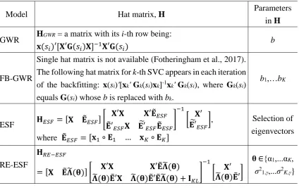
[Table 1 around here]
Table 1 summarizes p* for the study SVC models. Here, p*
GWR=tr[HGWR] inflates
when 𝐗′𝐆(𝑠𝑖)𝐗 is nearly singular. Singularity happens when the bandwidth is small and
most elements of G(si) take near zero values. In other words, small bandwidths introduce
over-fitting. The problem is serious if sub-samples are sparsely distributed around the site
si. Thus, GWR specified with an adaptive bandwidth (GWRa), which changes the kernel
window size in accordance with sample density, would be an effective tool to mitigate
this problem, where p*GWRa is likely to be smaller than p*GWR in many cases.
For GWR, it is important to note that the singularity of 𝐗′𝐆(𝑠𝑖)𝐗 changes
depending on the spatial scale of the predictor variables. If xk suggests small-scale spatial
18
suggests large-scale spatial variations, its variations within each kernel window can be
small. In the extreme case, if xk has uniform values across the window around site si, it is
exactly collinear with the intercept term within the window (i.e., suppose that x1
represents an intercept, the entries of the k-th row and column of 𝐗′𝐆(𝑠𝑖)𝐗 take exactly
the same values with the entries of the 1-st row and column. The resulting 𝐗′𝐆(𝑠𝑖)𝐗
becomes singular). The FB-GWR model, which calibrates the bandwidths implicitly
considering the scale of each xk, is valuable not only to control the varying scales of the
SVCs, but also to stabilize the SVC estimates (e.g., in the presence of collinearity).
Regarding ESF, forward eigenvector selection implicitly identifies the model
that maximizes accuracy, where p*
ESF =tr[HESF]. Given the fact that the Moran
eigenvectors describe coefficient patterns at different spatial scales, eigenvector selection
identifies the scale of spatial variation in each SVC set. p*
ESF increases as the number of
selected eigenvectors increases; it happens when SVCs have spatial variations in every
scale.
Unlike all of the above models, the effective number of parameters for the
RE-ESF model, p*
RE-ESF=tr[H RE-ESF], includes not just the scale parameters {α1,...αK}, but
also the variance parameters {σ21,γ,...σ2K,γ}. Different from GWR, FB-GWR and ESF
19
model is capable of stabilizing p*RE-ESF even if the SVCs tend have small-scale spatial
patterns (i.e., small α1,...αK) by decreasing the variance parameters.
3.
Monte Carlo simulation 1: scale vs. model complexity
3.1. Outline
This section objectively evaluates model complexity with p* values, while
varying the predictor variables and the scale parameters for the SVCs, and tests for which
cases the SVC models are unstable (i.e., investigates model limitation (a), from above).
For simplicity, we evaluate only cases where the spatial scale of variation for each set of
SVCs is the same. In other words, regression relationships are set to vary from the
small-scale to the large-small-scale, but always in the same fashion for each regression relationship in
the model. Thus FB-GWR is not analyzed here, as it simply defaults to standard GWR in
this instance.
For the Monte Carlo simulation, we assume a SVC model, 𝐲 = 𝛃0+ 𝐱1° 𝛃1+
𝐱2° 𝛃2+ 𝛆, where the predictor variables are generated from:
𝐱𝑘 = (1 − 𝑟𝑥)𝛆𝑥(𝑛𝑠)+ 𝑟𝑥𝐂(𝑏𝑥)𝛆𝑥(𝑠), (14)
where εx(ns)~ N(0, I) and εx(s)~ N(0, I). Here C(bk) is a matrix that row-standardizes a
20
where d(si, sj) is the Euclidean distance between sample sites si and sj. Spatial coordinates
of the sample sites are also allowed to vary, and are generated from standard normal
distributions. Thus, C(bk)εk is a spatial moving average process, and rx is the ratio of
spatially dependent variation to total variation in xk. Therefore, p* values for GWR,
GWRa, ESF, and RE-ESF are found while varying the parameters for the predictor
variables (see Table 2) and those for the SVCs (see Table 3). In each case, the p* values
of each model are evaluated 200 times. For ESF, [𝐱1∘ 𝐄1 … 𝐱𝐾∘ 𝐄𝐾], where Ek
consists of eigenvectors corresponding to positive eigenvalues, are candidates for the
variable selection step. These eigenvectors are also used in RE-ESF (i.e., E = Ek). The
ratio of the selected eigenvectors in ESF are given as described in Table 3.
Note that this section does not estimate SVCs through model fitting, but calculates
p* by simply substituting know parameters into p*=tr[H] (see, Table 1). For SVC
estimation accuracy, see Section 4.
[Table 2 around here]
[Table 3 around here]
21
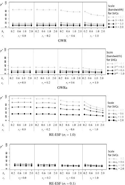
Figure 1 plots the mean estimated p* values for the SVC models arising from this
first Monte Carlo simulation experiment. Here the mean p*
GWR results suggest that GWR
(with a fixed bandwidth) is unstable when the SVCs have small-scale spatial variation (b
= 0.2). In other words, GWR could be stable unless the fixed bandwidth is inappropriately
small (i.e., b≠ 0.2).
Unlike the mean p*
GWR results, the mean p*GWRa results for GWRa (with its
adaptive bandwidth) are always relatively small across all values of b. At least from this
result, GWRa seems relatively stable compared to GWR. This is not surprising, given that
numerous empirical studies have suggested as much (e.g., Harris et al., 2010a). Only for
highly regular sample configurations is fixed bandwidth GWR usually recommended.
The drawback to GWRa, however, is that it implies non-stationary relationships
are operating within their own local region of dependence, whilst fixed bandwidth GWR,
ensures these regions are the same size everywhere, and thus provides more generalized
interpretations of the geographical process under study. For example, reporting that the
nature of the relationship between crime and unemployment depends only on incident
characteristics within a 2km radius of the crime scene is intuitively more informative than
reporting that this relationship depends only on the characteristics of the nearest 30
22
[Figure 1 around here]
In Figure 1, the mean p*
RE-ESF results are evaluated for cases with σk =0.1 and σk
=1.0, respectively. On the one hand, when σk =1.0, which implies weaker shrinkage, p*
RE-ESF takes large values. On the other hand, p*RE-ESF values are small across cases when
stronger shrinkage is imposed by σk =0.1. Thus, the RE-ESF estimates are relatively stable
even when the SVCs have local variation, but with a proviso that the σk parameter is
estimated appropriately. Furthermore, the mean p*
ESF values, which equal the number of
selected predictor variables, become {26.8, 50.7, 75.5, 98.3} in cases where the ratio of
selected eigenvectors equals {0.2, 0.4, 0.6, 0.8}, respectively. Considering the usefulness
of the shrinkage parameter, σk, in RE-ESF, regularized ESF (e.g., Seya et al., 2011) might
be useful to reduce p* ESF.
In summary, fixed bandwidth GWR can be very unstable when the bandwidth
of local parameter estimation is inappropriately small, and ESF tends to be unstable as
the number of selected eigenvectors increase. Conversely, GWRa is stable across both
small- and large-scale SVC processes, and RE-ESF is similarly stable, provided that σk is
23
Also observable from Figure 1 is that predictor variable, xk, with small-scale
spatial variations universally make all SVC models unstable. In contrast, in a context of
global spatial regression (e.g., spatial error model; e.g., LeSage and Pace, 2009), Paciorek
(2010) analytically showed that the coefficient estimates tend to be unstable if the spatial
scales of the predictor variables are larger than the scale of the residual spatial process.3
Thus, both small-scale xk and large-scale xk influence the reliability of the SVC estimates
for different reasons. The next section investigates the influence of all these instabilities
on the accuracy of the SVC estimates themselves, and tries to determine whether
small-scale xk or large-scale xk is more harmful in SVC estimation.
4.
Monte Carlo simulation 2: scale vs. SVC estimation accuracy
4.1. Outline
This section compares all six study SVC models (GWR, GWRa, GWR,
FB-GWRa, ESF and RE-ESF) though another Monte Carlo simulation experiment, where we
now assess the accuracy of the estimated SVCs in relation to the (known) simulated SVCs.
The synthetic data are generated from the following SVCs model:
𝐲 = 𝛃0+ 𝐱1° 𝛃1+ 𝐱2° 𝛃2+ 𝛆, 𝛆~𝑁(𝟎, 22𝐈), (15)
24
𝛃0 = 𝟏 + 𝐂(𝑏0)𝛆0, 𝛃1 = (−2)𝟏 + 3𝐂(𝑏1)𝛆1, 𝛃2 = (0.5)𝟏 + 𝐂(𝑏2)𝛆2,
where εk ~ N(0, I). The spatial variation in β1 is three times stronger than the spatial
variation in β0 and β2. We refer to β1 as a significant SVC process, whilst β0 and β2 are
considered to be insignificant SVC processes. Thus this simulation experiment
specifically investigates model limitation (b), from above. Following the previous section,
the predictor variables are generated from 𝐱𝑘 = (1 − 𝑟𝑥)𝛆𝑥(𝑛𝑠)+ 𝑟𝑥𝐂(𝑏𝑥)𝛆𝑥(𝑠) .
Parameters are estimated 200 times while varying parameter values, as summarized in
Table 4.
[Table 4 around here]
4.2.Results
The accuracy of each model’s SVC estimates is evaluated using root mean
squared error (RMSE), mean absolute error (MAE), and bias diagnostics. The results and
explanations of the MAE and bias diagnostics are given in the Appendix, whilst only the
RMSE results are presented here. The RMSE for estimated 𝛃̂𝐤 is given by the mean of
RMSE[𝛽̂𝑘(𝑠𝑖)], which is formulated as follows:
𝑅𝑀𝑆𝐸[𝛽̂𝑘(𝑠𝑖)] = √ 1
200 ∑ (𝛽𝑘(𝑠𝑖) − 𝛽̂𝑘(𝑠𝑖))2 200
𝑖𝑡𝑒𝑟=1
25
where 𝛽𝑘(𝑠𝑖) is the true SVC value generated from Eq. (15). To visualize the simulation
results effectively, we use 2-dimentional plots as presented in Figures 2 to 6. Here the
horizontal axis always denotes the RMSEs for RE-ESF, whose SVC estimation accuracy
has been shown to be relatively good across all cases in the ‘companion study’ of
Murakami et al. (2017), and the vertical axis denotes the RMSEs for one of the models
GWR, ESF, FB-GWR, GWRa, and FB-GWRa.
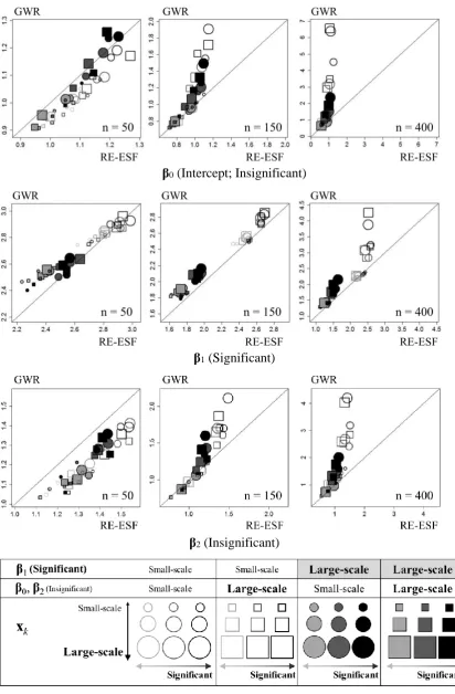
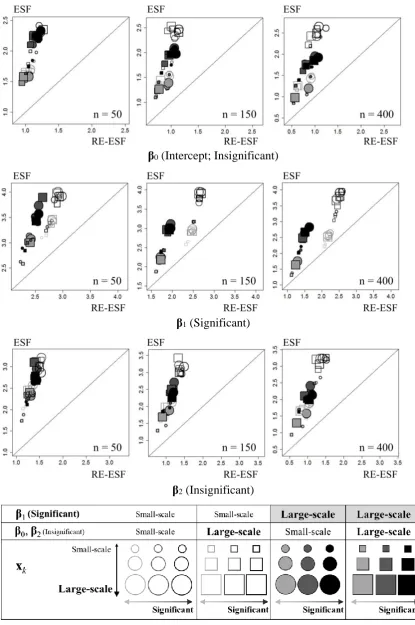
Figure 2 compares (fixed bandwidth) GWR with RE-ESF for SVC accuracy via
RMSE. Here, GWR provides more accurate SVCs than RE-ESF if the plot outputs are
concentrated in the bottom right triangle of each panel, while the estimated SVCs from
RE-ESF are more accurate if the plot outputs are in the top left triangle. Results clearly
demonstrates that the RMSEs from GWR are generally greater than those from RE-ESF,
and thus RE-ESF tends to be more accurate. This tendency is most conspicuous when the
significant SVC (β1) has the small-scale variables and xs has strong large-scale variations,
verifying that different scales of relationship non-stationarity need to be accounted for in
SVC models (which RE-ESF does, but GWR does not). This tendency is also substantial
for the largest sample size, when N = 400. By contrast, GWR can perform equally as well,
or better than, RE-ESF when N = 50. This is interesting, and may suggest that the smaller
26
different spatial scales. Furthermore, Páez et al. (2011) recommended using GWR only for large samples (N > 160), but these results suggest some value in GWR for small
samples. Figure 3 compares the coefficient RMSE results for ESF with RE-ESF, where it
is clear that ESF provides poorer levels of SVC estimation accuracy than RE-ESF, across
all nine scenarios. As with GWR (and as would be expected), ESF provides relatively
inaccurate SVCs in cases with small-scale variations in the significant SVC (β1) and
strong large-scale variations in xs. Although not shown graphically, by comparing Figure
2 with Figure 3, it is strongly suspected that GWR tends to perform better than ESF.
[Figure 2 around here]
[Figure 3 around here]
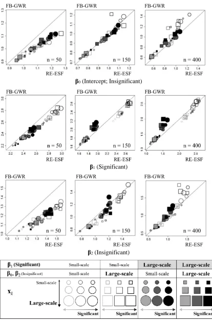
Figure 4 compares FB-GWR and RE-ESF, where, interestingly, unlike GWR, no
singular estimates appear from FB-GWR. Thus, GWR with multiple bandwidths (in this
FB-GWR form) appears to stabilize SVC estimates, and tentatively may provide a useful
alternative to a regularized GWR model in addressing local collinearity issues. As most
27
just as accurate as those from RE-ESF. Moreover, FB-GWR SVC estimates are more
accurate than RE-ESF when N = 50. This is because RE-ESF is a likelihood approach
relying on the law of large numbers. Conversely, the SVC estimates for FB-GWR tend to
be marginally less accurate than those from RE-ESF when xk have strong large-scale
spatial variations, and the significant SVC (β1) has small-scale variations (but for N = 150
and for N = 400, only).
[Figure 4 around here]
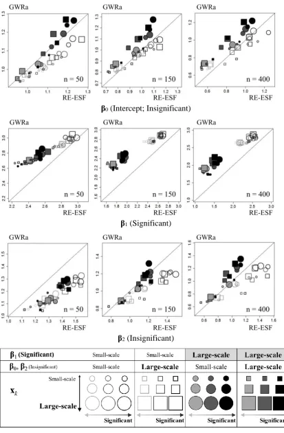
Figure 5 compares GWRa with RE-ESF for SVC accuracy. Somewhat
surprisingly, GWRa does not suffer from any singular fit, and RMSE values are greatly
reduced compared to the fixed bandwidth GWR results in Figure 2. The use of an adaptive
bandwidth appears to be a simple and efficient solution to stabilize GWR modeling,
although, in this case, stability may relate more to the effects of sample configurations
than to other influences. Conversely, GWRa provides much poorer levels of SVC
accuracy (than GWR and RE-ESF) for the significant small-scale SVC, β1. Furthermore,
the GWRa estimates for insignificant SVCs, β0 and β2, tend to be more accurate than that
28
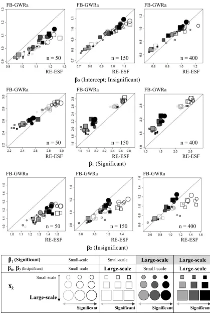
of accuracy to that found for RE-ESF for such cases. Figure 6 compares FB-GWRa with
RE-ESF for SVC accuracy. Here FB-GWRa appears to have similar coefficient accuracy
tendencies to those found with both FB-GWR (Figure 4) and GWRa (Figure 5), in relation
to RE-ESF. As would be expected, FB-GWRa is more accurate than GWRa for the
significant small-scale SVC, β1, where the FB-GWRa results are more compatible with
those from RE-ESF. Overall, FB-GWRa is found to estimate both weak and strong SVC
processes relatively accurately.
[Figure 5 around here]
[Figure 6 around here]
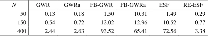
Finally, Table 5 compares average computational times for all six SVC models
for the three sample sizes of N = 50, 150, and 400. As expected, GWR and GWRa run the
fastest, as they are relatively simple. Considering the RMSE accuracy results, above, it is
recommended that GWRa would often be a sensible and pragmatic choice for very large
datasets. By contrast, FB-GWR and FB-GWRa are relatively slow due to their usage of
29
models would be an important research topic in the future, although some work in this
area is currently in progress (Lu et al. in review). The ESF model is also slow because it
requires stepwise eigenvector selection. By contrast, RE-ESF is as fast as GWR and
GWRa, despite the fact that it estimates each spatial scale of each set of SVCs (i.e.,
RE-ESF is multi-scale). This is because the computational complexity for optimizing the
scale parameters is only O(L3K3), which is independent of sample size. Note also that the
cost for eigen-decomposition for RE-ESF, which is severe when N is large, can be
lightened dramatically by an approximation proposed by Griffith (2000), which is for
regular lattice data, or Murakami and Griffith (2017). Thus, RE-ESF is also recommended
for very large datasets, and should be preferred to GWRa when relationships are not only
expected to vary locally, but also across different spatial scales.
[Table 5 around here]
5.
Concluding remarks
The study summarized in this paper investigated the influence of scale on SVC
modeling, where relationships between the response and predictor not only operate locally,
30
standard GWR provides poor SVC estimates, when some SVCs vary at a small-scale
whilst others vary at a large-scale. By contrast, a multi-scale GWR model in FB-GWR
provides SVC estimates that are relatively accurate for such processes. Interestingly,
differences in SVC estimation accuracy, and model stability, also depend on whether fixed
distance or adaptive distance kernel bandwidths are specified for GWR or for FB-GWR,
where adaptive ones should in general be preferred.
GWR and FB-GWR are examples of local approaches to SVC modelling, whilst
ESF and RE-ESF are both global approaches. Here RE-ESF is a regularized ESF model
that is designed to capture scale dependencies in local relationships, just as FB-GWR is.
The RE-ESF is shown to more accurately estimate such multi-scale SVC processes in
comparison to not only ESF, but also to GWR. RE-ESF is also shown to be a more stable
model than ESF or GWR. Both FB-GWR and RE-ESF are found to provide the most
accurate estimates of the SVC processes generated in the simulation experiment, but
where RE-ESF is shown to be the most computationally efficient, and thus more suitable
for very large datasets. Overall, the results strongly indicate that future SVC studies need
to pay more attention to issues of spatial scale, and investigate with a FB-GWR or
RE-ESF model, especially considering it is entirely unrealistic for each set of SVCs to operate
31
Still, there are some remaining issues, where future work on the analytic
properties of spatial scale and SVC estimates could follow that of Paciorek (2010), where
only the effects on stationary regression coefficients were investigated. Such studies
would help in understanding the scale problem more deeply, and possibly enable the
establishment of a local/global indicator of scale dependence for SVCs. Extensions
should also consider: (i) non-Gaussian data modeling (Atkinson et al., 2003; Griffith,
2002; 2004; Nakaya et al., 2005), (ii) spatiotemporal modeling (Huang et al., 2010;
Griffith, 2012; Fotheringham et al., 2015), (iii) spatial prediction (Harris et al., 2010b;
2011; Griffith, 2013), (iv) spatial interaction modeling (Nakaya, 2001; Kordi and
Fotheringham 2016; Griffith et al., 2017), and (v) the mitigation of the modifiable areal
unit problem (Fotheringham et al., 2002; Murakami and Tsutsumi, 2015).
Acknowledgements
This study was jointly funded by the JSPS KAKENHI Grant Numbers
17K12974 and 17K14738; projects from the National Natural Science Foundation of
China [NSFC: 41401455 and U1533102]. Work was also supported by a UK
Biotechnology and Biological Sciences Research Council grant (BBSRC
32
Reference
- Anselin, L. (2010). Thirty years of spatial econometrics. Papers in regional science, 89(1), 3-25.
- Anselin, L., & Rey, S. (1991). Properties of tests for spatial dependence in linear regression models. Geographical analysis, 23 (2), 112-131.
- Assunção RM (2003) Space varying coefficient models for small area data.
Environmetrics 14:453-473
- Atkinson, P. M., German, S. E., Sear, D. A., & Clark, M. J. (2003). Exploring the relations between riverbank erosion and geomorphological controls using geographically weighted logistic regression. Geographical Analysis, 35 (1), 58-82. - Bitter, C., Mulligan, G. F., & Dall’erba, S. (2007). Incorporating spatial variation in
housing attribute prices: a comparison of geographically weighted regression and the spatial expansion method. Journal of Geographical Systems, 9 (1), 7-27.
- Bárcena, M. J., Menéndez, P., Palacios, M. B., & Tusell, F. (2014). Alleviating the effect of collinearity in geographically weighted regression. Journal of Geographical
Systems, 16 (4), 441-466.
- Bishop, C. M. (2006). Pattern recognition and machine learning. Springer.
33
Regression: A Method for Exploring Spatial Nonstationarity. Geographical Analysis,
28 (4), 281-298.
- Brunsdon C, Fotheringham AS, Charlton ME (1998) Geographically weighted
regression - modelling spatial non-stationarity. Journal of the Royal Statistical Society,
Series D-The Statistician 47(3):431-443
- Brunsdon, C., Fotheringham, A.S., and Charlton, M. (1999). Some notes on
parametric significance tests for geographically weighted regression. Journal of
Regional Science, 39 (3), 497–524.
- Brunsdon, C., McClatchey, J., & Unwin, D. J. (2001). Spatial variations in the average
rainfall–altitude relationship in Great Britain: an approach using geographically
weighted regression. International journal of climatology, 21 (4), 455-466.
- Casetti, E. (1972). Generating models by the expansion method: applications to
geographical research. Geographical analysis, 4 (1), 81-91.
- Casetti, E., & Jones III, J. P. (1992). An introduction to the expansion method and to
its applications. Applications of the expansion method, 1-9.
- Cho, S-H., Lambert, D.M., Chen Z (2010). Geographically weighted regression
bandwidth selection and spatial autocorrelation: an empirical example using Chinese
agriculture data. Applied Economics Letters, 17, 767-772.
34
- Farber, S., & Páez, A. (2007). A systematic investigation of cross-validation in GWR
model estimation: empirical analysis and Monte Carlo simulations. Journal of
Geographical Systems, 9 (4), 371-396.
- Finley, A. O. (2011). Comparing spatially‐varying coefficients models for analysis of
ecological data with non‐stationary and anisotropic residual dependence. Methods in
Ecology and Evolution, 2 (2), 143-154.
- Fotheringham, A. S., Brunsdon, C., & Charlton, M. (2002). Geographically weighted
regression: the analysis of spatially varying relationships. John Wiley & Sons.
- Fotheringham, A. S., Crespo, R., & Yao, J. (2015). Geographical and temporal
weighted regression (GTWR). Geographical Analysis, 47 (4), 431-452.
- Fotheringham, A. S., & Oshan, T. M. (2016). Geographically weighted regression and
multicollinearity: dispelling the myth. Journal of Geographical Systems, 18 (4),
303-329.
- Fotheringham, A.S., Yang, W., & Kang, W. (2017). Multiscale Geographically
Weighted Regression (MGWR). Annals of the American Association of Geographers
DOI: 10.1080/24694452.2017.1352480
- Gamerman D, Moreira ARB, Rue H (2003). Space-varying regression models:
35
- Gelfand, A. E., Kim, H. J., Sirmans, C. F., & Banerjee, S. (2003). Spatial modeling
with spatially varying coefficient processes. Journal of the American Statistical
Association, 98 (462), 387-396.
- Gollini, I., Lu, B., Charlton, M., Brunsdon, C., & Harris, P. (2015). GWmodel: an R
package for exploring spatial heterogeneity using geographically weighted models.
Journal of Statistical Software, 63(17), 1-50.
- Griffith, D.A. (2000). Eigenfunction properties and approximations of selected
incidence matrices employed in spatial analyses. Linear Algebra & Its Applications,
321 (1-3), 95-112.
- Griffith, D.A. (2002). A spatial filtering specification for the auto-Poisson model.
Statistics & Probability Letters, 58 (3), 245-251.
- Griffith, D. A. (2003). Spatial autocorrelation and spatial filtering: gaining
understanding through theory and scientific visualization. Springer Science &
Business Media.
- Griffith, D. A. (2008). Spatial-filtering-based contributions to a critique of
geographically weighted regression (GWR). Environment and Planning A, 40 (11),
2751-2769.
36
Environment and Planning A, 36 (10), 1791-1811.
- Griffith, D.A. (2012). Space, time, and space-time eigenvector filter specifications
that account for autocorrelation. Estadística Española, 54 (177), 7-34.
- Griffith, D.A. (2013). Estimating missing data values for georeferenced Poisson
counts. Geographical Analysis, 45 (3), 259-284.
- Griffith, D.A. (2017). Some robustness assessments of Moran eigenvector spatial
filtering. Spatial Statistics, in press.
- Griffith, D.A., Fischer, D.M., & LeSage, J.P. (2017). The spatial autocorrelation
problem in spatial interaction modelling: a comparison of two common solutions.
Lettersin Spatial and Resource Sciences, 10 (1), 75-86.
- Harris P, Fotheringham AS, & Juggins S (2010a). Robust geographically weighed
regression: a technique for quantifying spatial relationships between freshwater
acidification critical loads and catchment attributes. Annals of the Association of
American Geographers 100(2): 286-306
- Harris, P., Fotheringham, A. S., Crespo, R., & Charlton, M. (2010b). The use of
geographically weighted regression for spatial prediction: an evaluation of models
using simulated data sets. Mathematical Geosciences, 42 (6), 657-680.
37
extensions of the geographically weighted regression model when used as a spatial
predictor. Stochastic environmental Research and Risk assessment, 25 (2), 123-138.
- Harris P, Brunsdon C, Lu B, Nakaya T, Charlton M (2017) Introducing bootstrap
methods to investigate coefficient non-stationarity in spatial regression models.
Spatial Statistics 21: 241-261
- Helbich, M., & Griffith, D. A. (2016). Spatially varying coefficient models in real
estate: Eigenvector spatial filtering and alternative approaches. Computers,
Environment and Urban Systems, 57, 1-11.
- Hu, M, Li, Z., Wang, J., Jia, L., Lai, S., Guo, Y., Zhao, D., Yang, W. (2012).
Determinants of the incidence of hand, foot and mouth disease in China using
geographically weighted regression models. PLoS ONE 7(6): e38978.
doi:10.1371/journal.pone.0038978
- Huang, B., Wu, B., & Barry, M. (2010). Geographically and temporally weighted
regression for modeling spatio-temporal variation in house prices. International
Journal of Geographical Information Science, 24 (3), 383-401.
- Kordi, M. & A. S. Fotheringham (2016) Spatially Weighted Interaction Models
(SWIM). Annals of the American Association of Geographers, 106(5), 990-1012.
38
driving forces behind deforestation in the state of Mexico (Mexico) using
geographically weighted regression. Applied Geography, 30 (4), 576-591.
- Leong, Y. Y., & Yue, J. C. (2017). A modification to geographically weighted
regression. International Journal of Health Geographics, 16 (1), 11.
- LeSage, J. P. & Pace, R. K. (2009). Introduction to spatial econometrics. CRC press.
- Lloyd, C. D. (2010). Local models for spatial analysis. CRC press.
- Lu, B., Charlton, M., Harris, P., Fotheringham, A. S. (2014a). Geographically
weighted regression with a non-Euclidean distance metric: a case study using hedonic
house price data. International Journal of Geographical Information Science, 28(4),
660-681.
- Lu, B., Harris, P., Charlton, M., & Brunsdon, C. (2014b). The GWmodel R package:
further topics for exploring spatial heterogeneity using geographically weighted
models. Geo-spatial Information Science, 17 (2), 85-101.
- Lu, B., Brunsdon, C., Charlton, M., & Harris, P. (2017). Geographically weighted regression with parameter-specific distance metrics. International Journal of
Geographical Information Science, 31 (5), 982-998.
39
Planning A 38:587-598
- Mei, C.-L., Xu, M. & Wang, N. (2016) A bootstrap test for constant coefficients in
geographically weighted regression models. International Journal of
Geographical Information Science, 30, 1622-1643.
- Murakami, D. (2017). spmoran: an R package for Moran's eigenvector-based spatial
regression analysis. Arxiv, 1703.04467.
- Murakami, D., & Griffith, D. A. (2015). Random effects specifications in eigenvector
spatial filtering: a simulation study. Journal of Geographical Systems, 17 (4),
311-331.
- Murakami, D., & Griffith, D. A. (2017). Eigenvector spatial filtering for large data
sets: fixed and random effects approaches. ArXiv,1702.06220.
- Murakami, D., & Tsutsumi, M. (2015). Area-to-point parameter estimation with
geographically weighted regression. Journal of Geographical Systems, 17 (3),
207-225.
- Murakami, D., Yoshida, T., Seya, H., Griffith, D. A., & Yamagata, Y. (2017). A Moran
coefficient-based mixed effects approach to investigate spatially varying relationships.
Spatial Statistics, 19, 68-89.
40
weighted regression approach, GeoJournal 53, 347-358.
- Nakaya, T. (2015). Geographically weighted generalised linear modeling. Brunsdon,
C. and Singleton, A. eds. Geocomputation: A Practical Primer', Sage Publication,
201-220.
- Nakaya, T., Fotheringham, A. S., Brunsdon, C., & Charlton, M. (2005).
Geographically weighted Poisson regression for disease association mapping.
Statistics in medicine, 24 (17), 2695-2717.
- Ndiath, MN, Cisse, B., Ndiaye, J.L., Gomis, J.F., Bathiery, O., Dia, A.T., Gaye, O.,
Faye, B. (2015). Application of geographically-weighted regression analysis to assess
risk factors for malaria hotspots in Keur Soce health and demographic surveillance
site. Maleria Journal, 14:463.
- Oshan, T. M., & Fotheringham, A. S. A (2017). Comparison of spatially varying
regression coefficient estimates using geographically weighted and spatial‐filter‐
based techniques. Geographical Analysis, DOI: 10.1111/gean.12133.
- Paciorek, C. J. (2010). The importance of scale for spatial-confounding bias and
precision of spatial regression estimators. Statistical science: a review journal of the
Institute of Mathematical Statistics, 25 (1), 107.
41
estimation: an empirical comparison of modelling techniques. Urban Studies, 45 (8), 1565-1581.
- Páez, A., Farber, S., & Wheeler, D. (2011). A simulation-based study of geographically weighted regression as a method for investigating spatially varying relationships. Environment and Planning A, 43 (12), 2992-3010.
- Sampson PD, Damian D, Guttorp P (2001) Advances in modeling and inference for
environmental processes with nonstationary spatial covariance. NRCSE-TRS No 61,
National Research Centre for Statistics and the Environment Technical Report Series,
2001
- Seya, H., Murakami, D., Tsutsumi, M., & Yamagata, Y. (2015). Application of LASSO to the Eigenvector Selection Problem in Eigenvector‐based Spatial Filtering.
Geographical Analysis, 47 (3), 284-299.
- Wheeler, D. C. (2007). Diagnostic tools and a remedial method for collinearity in geographically weighted regression. Environment and Planning A, 39 (10), 2464-2481.
- Wheeler, D. C. (2009). Simultaneous coefficient penalization and model selection in geographically weighted regression: the geographically weighted lasso. Environment
42
- Wheeler, D. C., & Calder, C. A. (2007). An assessment of coefficient accuracy in linear regression models with spatially varying coefficients. Journal of Geographical
Systems, 9 (2), 145-166.
- Wheeler, D. C., & Waller, L. A. (2009). Comparing spatially varying coefficient models: a case study examining violent crime rates and their relationships to alcohol outlets and illegal drug arrests. Journal of Geographical Systems, 11 (1), 1-22. - Wheeler, D., & Tiefelsdorf, M. (2005). Multicollinearity and correlation among local
regression coefficients in geographically weighted regression. Journal of
Geographical Systems, 7 (2), 161-187.
- Yang W, Fotheringham AS, Harris P (2011) Model selection in GWR: the development of a flexible bandwidth GWR. Geocomputation 2011, London, UK
- Yang W, Fotheringham AS, Harris P (2012) An extension of Geographically Weighted Regression with Flexible Bandwidths. GISRUK 2012, Lancaster, UK
- Yang, W. (2014). An extension of geographically weighted regression with flexible
43
Table 1: The hat matrix, H, of the study SVC models, where p*= tr[H].
Model Hat matrix, H Parameters
in H
GWR HGWR = a matrix with its i-th row being:
𝐱(𝑠𝑖)′[𝐗′𝐆(𝑠𝑖)𝐗]−1𝐗′𝐆(𝑠 𝑖)
b
FB-GWR
Single hat matrix is not available (Fotheringham et al., 2017).
The following hat matrix for k-th SVC appears in each iteration
of the backfitting: x(si)'[xk'Gk(si)xk]-1xk'Gk(si), where Gk(si) equals G(si) whose b is replaced with bk.
b1,…bK
ESF 𝐇𝐸𝑆𝐹 = [𝐗 𝐄̃𝐸𝑆𝐹] [
𝐗′𝐗 𝐗′𝐄̃𝐸𝑆𝐹 𝐄̃′𝐸𝑆𝐹𝐗 𝐄′̃𝐸𝑆𝐹𝐄̃𝐸𝑆𝐹]
−1 [ 𝐗′
𝐄′̃𝐸𝑆𝐹],
where 𝐄̃𝐸𝑆𝐹 = [𝐱1∘ 𝐄1 … 𝐱𝐾∘ 𝐄𝐾]
Selection of eigenvectors RE-ESF 𝐇𝑅𝐸−𝐸𝑆𝐹 = [𝐗 𝐄̃𝚲̃(𝛉)] [ 𝐗′𝐗 𝐗′𝐄̃𝚲̃(𝛉) 𝚲̃(𝛉)𝐄̃′𝐗 𝚲̃(𝛉)𝐄̃′𝐄̃𝚲̃(𝛉) + 𝐈𝐾𝐿 ] −1 [ 𝐗′ 𝚲̃(𝛉)𝐄̃′]
θ ∈{α1,...αK,
σ2
1,γ,...σ2K,γ}
Table 2: Parameter settings for predictor variables: xk
Parameter Notation Case
Sample size N 400
Bandwidth bx {0.0, 0.2, 0.6, 1.0}
Ratio of spatial variation rx {0.2, 0.6, 1.0, 2.0}
Table 3: Parameter settings for SVCs: βk
Model Parameter Notation Case
GWR Bandwidth b {0.2, 0.6, 1.0, 2.0}
GWRa Adaptive bandwidth bad {0.1, 0.3, 0.5, 1.0}
ESF Ratio of predictor variables being selected q {0.2, 0.4, 0.6, 0.8}
RE-ESF
Scale αk {0.2, 0.6, 1.0, 2.0}
44
Table 4: Parameter settings in 144 (3×4×3×4) cases.
Parameter Notation Case
Sample size N {50, 150, 400}
Bandwidth for {β0. β1, β2} (b0, b1, b2)
{(0.2, 0.2, 0.2), (1.0, 0.2, 1.0),
(0.2, 1.0, 0.2), (1.0, 1.0, 1.0)}
Bandwidth for xk bx {0.2, 0.6, 1.0}
Ratio of spatial variation in xk rx {0.0, 0.4, 0.8, 1.0}
Table 5: Average computational time in seconds.
N GWR GWRa FB-GWR FB-GWRa ESF RE-ESF
50 0.13 0.18 1.50 10.31 1.49 0.29
150 0.54 0.72 12.02 12.96 10.52 0.77
45 GWR
GWRa
RE-ESF (σγ = 1.0)
RE-ESF (σγ = 0.1)
Figure 1: Mean effective number of parameters, p*, with respect to the scale of the SVCs. In each panel, lighter lines represent p*s
46
β0 (Intercept; Insignificant)
β1 (Significant)
β2 (Insignificant)
47
β0 (Intercept; Insignificant)
β1 (Significant)
β2 (Insignificant)
48
β0 (Intercept; Insignificant)
β1 (Significant)
β2 (Insignificant)
49
β0 (Intercept; Insignificant)
β1 (Significant)
β2 (Insignificant)
50
β0 (Intercept; Insignificant)
β1 (Significant)
β2 (Insignificant)