Article
Using MODIS Data to Predict Regional Corn Yields
Ho-Young Ban 1, Kwang Soo Kim 1, No-Wook Park 2 and Byun-Woo Lee 1,3,*
1 Department of Plant Science, College of Agriculture and Life Sciences, Seoul National University, 1 Gwanak-ro, Gwanak-gu, Seoul 08826, Korea; [email protected] (H.-Y.B.); [email protected] (K.S.K.) 2 Department of Geoinformatic Engineering 4-311 & 4-309, Inha University, 100 Inha-ro, Nam-gu, Incheon
402-751, Korea; [email protected]
3 Research Institute of Agriculture and Life Sciences, Seoul National University, 1 Gwanak-ro, Gwanak-gu, Seoul 08826, Korea
* Correspondence: [email protected]; Tel.: +82-2-880-4544
Abstract: A simple approach was developed to predict corn yields using the MoDerate Resolution Imaging Spectroradiometer (MODIS) data product from two geographically separate major corn crop production regions: Illinois, USA and Heilongjiang, China. The MOD09A1 data product, which are 8-day interval surface reflectance data, were obtained from day of the year (DOY) 89 to 337 to calculate the leaf area index (LAI). The sum of the LAI from early in the season to a given date in the season [end of DOY (EOD)] was well fitted to a logistic function and represented seasonal changes in leaf area duration (LAD). A simple phenology model was derived to estimate the dates of emergence and maturity using the logistic function parameters b1 and b2, which represented the rate of increase in LAI and the date of maximum LAI, respectively. The phenology model predicted emergence and maturity dates fairly well, with root mean square error (RMSE) values of 6.3 and 4.9 days for the validation dataset, respectively. Two simple linear regression models (YP and YF) were established using LAD as the variable to predict corn yield; the yield model (YP) used LAD from predicted emergence to maturity, and the yield model (YF) used LAD for a predetermined period from DOY 89 to a particular EOD. When state/province corn yields for the validation dataset were predicted at DOY 321, near completion of the corn harvest, the YP model performed much better than the YF model, with RMSE values of 0.68 t/ha and 0.66 t/ha for Illinois and Heilongjiang, respectively. The YP model showed a similar or better performance, even for the much earlier yield prediction at DOY 257, compared to that of the YF model. In conclusion, the phenology and yield models were developed based only on logistic changes in remote sensing-derived LAD, and predicted phenological dates and corn yields with considerable accuracy and precision for the two regions selected for this study. However, these models must be examined for spatial portability in more diverse agro-climatic regions.
Keywords: MODIS; yield; phenology; LAD; logistic function
1. Introduction
Crop production has a direct effect on year-to-year national and international economics and the food supply [1]. The ability to predict crop yield would help government agencies develop food security and trade policies [2-4]. Non-governmental organizations would also benefit from reliable crop yield predictions by allowing decisions to be made regarding food aid [5].
Monitoring crop growth in fields can be used to predict crop yield reliably. For example, the LAI during the growing season is a key variable used to predict crop biomass and yield [6,7]. LAD, which is integrated with the LAI value over time, has also been suggested to have a strong correlation with dry matter production and grain yield [8,9].
intercepted photosynthetically active radiation have been provided through the MODIS database [12-14].
The application of remote sensing data products enables reliable and timely predictions of crop yields [15]. These data products are based on different vegetation indices and have been used to assess quantitative crop growth, e.g., LAI and biomass. For example, the wide dynamic range vegetation index (WDRVI) and the enhanced vegetation index have been used to predict LAI in agricultural croplands [16-19]. Qualitative changes in crop growth, such as crop phenology, have also been assessed using remote sensing data products [20-22]. Assessing crop phenology helps with the estimates needed for crop management, and is useful to reliably predict crop yield because the effects of environmental conditions on crop yield differ by growth stage [23].
Predicting crop growth and yield using remote sensing data products often depends on an empirical approach [24]. Although simple models to predict crop yield can be developed from such an approach [10,25], it is likely that the spatial portability of the model would be limited. Sophisticated approaches requiring additional data have also been developed to improve predictions of crop growth and yield [26,27]. Lobell [26] used photosynthetically active radiation (PAR), the fraction of PAR, radiation use efficiency, and the harvest index as input variables. Nevertheless, it is preferable to develop a crop yield prediction model with wide spatial portability using a small dataset [28].
The objectives of this study were to develop a simple approach to predict crop phenology and yield using a minimum set of remote sensing data products and to examine the spatial portability of the simple method. Reliably predicting corn yield could help assess the socioeconomic impact on food production at regional and global scales. This study focused on predicting corn yield in major production areas of the USA and China.
2. Materials and Methods
2.1. Study area
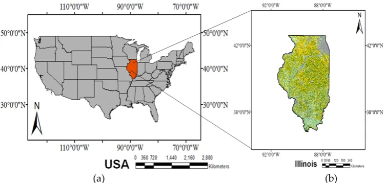
A simple approach using remote sensing data products was developed to predict crop yields in major crop production areas in the USA and China, where varieties and cultivation methods differ considerably. Illinois, USA (40°0′0″N, 89°0′0″W) (Figure 1a) and Heilongjiang Province, China (47°50′0″N, 127°40′0″E) (Figure 2a) were selected as the regions of interest. Illinois and Heilongjiang are located on opposite sides of the Earth. The latitude of Heilongjiang is higher than that of Illinois. Accordingly, environmental conditions (e.g., temperature, precipitation, and solar radiation) differ between the sites. Annual mean temperature in Illinois is approximately 10 °C, while in Heilongjiang it is −4 °C to 4 °C. These different environmental conditions are why different crop varieties and cultivation methods are used at the two sites [29].
(a) (b)
(a) (b)
Figure 2. Map of the China showing the location of Heilongjiang (a) and crop cover data for Heilongjiang in 2012 (b) (Corn is indicated by yellow).
The corn production area and the quantity of corn produced as a proportion of the national total in Illinois were about 32% and 15% in 2013, respectively. The corresponding values in Heilongjiang were about 9% and 12%, respectively.
2.2. Crop yield and phenology data
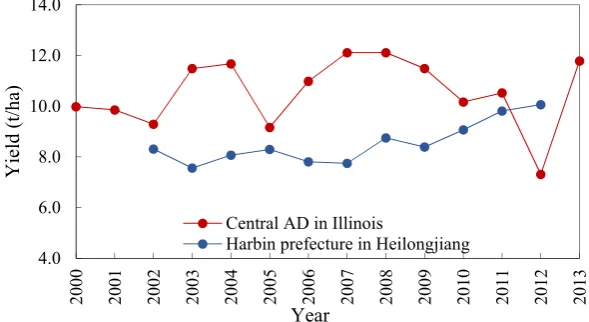
Corn yields in Illinois and Heilongjiang (Figure 3) were obtained from official reports provided by statistical services in each country. In Illinois, crop yields from 2000 to 2013 were gathered from the National Agricultural Statistics Service (NASS) by agricultural district (AD). Crop area and total production of each crop were also obtained from the NASS by county and state. The unit system for crop yield in Illinois was converted from “bushels per acre” to “kilograms per hectare” to fit the unit system used in Heilongjiang.
Yields and planted area for 2002 to 2012 in Heilongjiang Province were collected from the Heilongjiang Statistical Yearbook by prefecture and province. Corn yields in Heihe and Daxinganling prefectures in Heilongjiang Province were excluded from the calculation to minimize computing resources because mean corn production was considerably lower than in other areas of the province.
Figure 3. Reported corn yields from 2000 to 2013 in the central AD, Illinois and from 2002 to 2012 in Harbin prefecture, Heilongjiang.
4.0 6.0 8.0 10.0 12.0 14.0
2000 2001 2002 2003 2004 2005 2006 2007 2008 2009 2010 2011 2012 2013
Yield (t/ha)
Year
Central AD in Illinois
Corn phenology data were gathered for Illinois by AD. Weekly data were obtained from the NASS-Illinois Field Office (IFO). These data were only available for five ADs (northwest, northeast, central, western, and eastern districts) between 2003 and 2012. The dates of emergence and maturity were obtained for corn. Because of the limited availability of phenology data in Heilongjiang Province, a model was established and validated to predict the phenological stages using data only for the ADs in Illinois, USA and was applied to predict the phenological stages in Heilonjiang, China.
The phenology data were used to evaluate the reliability of a model to predict phenological changes of the crop using remote sensing data. The date on which a given phenological stage reached 50% in the study area, e.g., an AD, was used to represent when a phenological stage occurred. It was assumed that the proportion of area in a given stage would increase linearly over a two-week period. The weekly data for the proportion of area where the crop was at the phenological stage of interest were collected from the NASS-IFO. Those weekly data were used to compare the estimated dates on which a phenological stage occurred in the AD. For example, the day on which the corn crop reached a phenological stage was determined from a linear interpolation between the weekly proportion of area for the given phenological stage.
2.3. Crop cover data
Corn crop cover data were obtained to identify the area where a given crop was grown. Crop cover data (Figure 1b) were collected from 2000 to 2013 in Illinois using the NASS database (https://www.nass.usda.gov/Research_and_Science/Cropland/SARS1a.php). The crop cover data in China (Figure 2b) were generated using remote sensing [30]. Crop areas were identified from the MODIS Land cover type product (MCD12Q1). Major crops, including corn, within the crop areas were classified using a maximum likelihood classifier and time-series MODIS 16-day NDVI dataset (MOD 13). Crop cover data, which have a spatial resolution of 250 m, were subjected to reprojection using ENVI (ExelisVIS: Exelis Visual Information Solutions, Boulder, CO, USA). The projections of the crop cover maps in both regions were converted using a Universal Transverse Mercator (UTM) projection and WGS-84 coordinates at a 1 km spatial resolution.
2.4. Calculating the LAI using a remote sensing data product
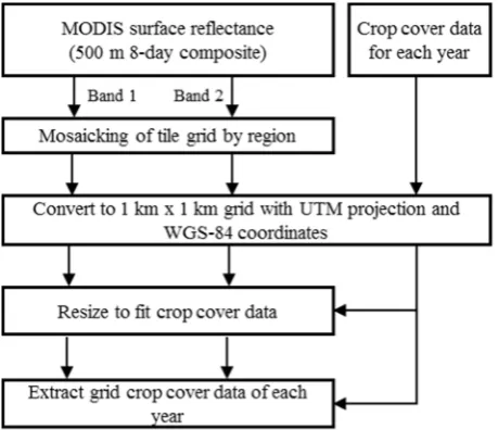
The MODIS surface reflectance data product was used to calculate the LAI and predict crop yields (Figure 4). The MOD09A1 data, which have a spatial resolution of 500 m, were obtained for 2000–2013. These data were downloaded from Reverb, which is a web-based remote sensing data portal operated by the National Aeronautics and Space Administration (http://modis.gsfc.nasa.gov/). The h10v04, h10v05, h11v04, and h11v05 tiled grid data for Illinois were collected from DOY 89 to 329. The h26v04 and h27v04 tiled grid data were obtained for the same period in Heilongjiang.
Nguy-Robertson et al. [31] suggested that the combined vegetation index (CVI) is more accurate than a single vegetation index set to estimate LAI. Instead of using the LAI products from the MODIS data, the LAI value was calculated for corn as follows [31]:
LAI = (SR − 1.0)/3.5 ,(NDVI − 0.28)/0.28 , NDVI ≤ 0.7NDVI > 0.7 (1)
where NDVI and SR are the normalized difference vegetation index [32] and simple ratio [33], respectively. NDVI and SR were determined as follows:
NDVI = (NIR − red)/(NIR + red) (2)
where NIR and red indicate the near-infrared and red band spectra.
The NIR and red band reflectance maps were prepared using a series of data tools (Figure 4). First, Interface Description Language (IDL; ExelisVIS) was used to mosaic all tiled data into a single dataset. The mosaic data projection was converted to a UTM projection at 1 km spatial resolution and WGS-84 geographic latitude and longitude projection using IDL, which applies the triangulation wrap and nearest neighbor resampling methods. FWTools, which is a collection of open-source GIS applications, was used to georeference the reflectance maps. Gridded data for the region of interest were prepared by extracting the reflectance data for the given extent by year using MATLAB (MathWorks Inc., Natick, MA, USA), which is a multi-paradigm numerical computing environment and fourth-generation programming language.
Figure 4. Data-flow diagram of the surface reflectance and crop cover data used to standardize the data.
Cropland was identified using the proportion of crop cover in each pixel of the MODIS product using a mixed problem and low resolution [34,35]. Crop cover data of the cropland data layer were overlapped with the MODIS data to calculate the percentage of pixels where a given crop was grown in the research region. It was assumed that the crop of interest would be grown within pixels where the percentage of corn was > 60% and > 90%. Although identifying a crop using the percentage of crop cover could be used for the pure growing region of the crop, a percentage value was not set for the identification method, so the mixed problem differed by region and crop. This method can cause problems when integrating from a smaller to a larger scale due to the pixels excluded below the threshold percentage. We attempted to identify the corn cultivation region according to the data standardization procedure described in Figure 4. The number of identified pixel in Illinois and Heilongjiang were approximately 610,000 and 860,000, respectively.
2.5. Estimating phenological dates
A logistic function was used to represent the temporal change in the sum of LAI as follows (Equation (5)):
( ) =
1.0 + exp[− ( − )] (4)
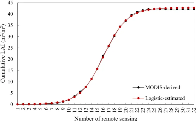
where b1, b2, and b3 represent the rate of LAI growth, the date on which the LAI would be maximum, and the cumulative LAI at physiological maturity, respectively, and t indicates days after planting. Although it would be preferable to determine the t-value as the date after the exact planting date, it was challenging to obtain this date in each grid cell. Because a logistic function was used in Equation (4), it was assumed that the t-value could be determined using a date earlier than the actual planting date. In this study, DOY 89 was used as the beginning of the cropping season, which was the date prior to the actual planting for the regions of interest. The order of the remote sensing data products since DOY 89 was used to determine the t-value and conveniently estimate the logistic function parameters. For example, t was 2 when data production on DOY 97 was used for Equation (4). The simplex method [36] was used to determine the parameter values of Equation (4) for each grid cell. The sum of the LAI derived from the MODIS product until a given date was compared with that obtained from Equation (4). The LAI values from 89 to 337 DOY were accumulated at eight-day intervals for each grid cell at a 1-km resolution. The sum of the square error between the observed and simulated values of cumulative LAI was minimized to obtain parameter values for b1, b2, and b3 in the simplex algorithm.
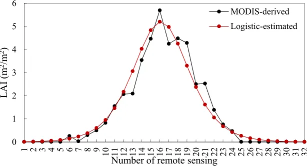
Figure 5. MODIS-derived and logistic-estimated cumulative LAI for corn in Illinois. The X-axis denotes the order of the dates for the remote sensing data product. For example, products for DOY 89 and 97 are indicated by 1 and 2, respectively.
The dates of emergence and maturity were estimated using a simple empirical equation (Equation (5)). It was assumed that date DP for a given phenology P could be determined using the b1 and b2 values, which represent the rate of LAI increase and the date of maximum LAI at a given site, respectively, as follows:
D = b + τ + ρ /b (5)
where τ and ρ are empirical coefficients, τ represents the overall time difference between the date of the maximum LAI and a given phenological stage P, ρ represents the impact of the increase in LAI on phenological change over time, and τ and ρ were estimated using the simplex method. The NASS-derived dates for a given phenology were compared with those obtained from Equation (5).
0 5 10 15 20 25 30 35 40 45
1 2 3 4 5 6 7 8 9 10 11 12 13 14 15 16 17 18 19 20 21 22 23 24 25 26 27 28 29 30 31 32
Cu
m
ulativ
e LAI
(m
2/m 2)
Number of remote sensing
MODIS-derived
2.6. Corn yield predictions
Daily LAI values were determined from emergence to maturity. The derivatives of Equation (4) on a given date represented the LAI on that date.
LAI = ∙ ∙ exp[− ( − )]
1.0 + exp[− ( − )] (6)
Daily changes in the LAI (Figure 6) were determined for each grid cell. Daily LAD was also determined from the date of emergence to that of maturity, as follows [37]:
LAD = ( + )
2 (7)
where LAId is the LAI value on d. The sum of the LAD values was obtained for the growing periods, e.g., from the emergence to the maturity date, for each grid cell. Then, the sum of those values was averaged by region, e.g., AD and prefecture in a season as follows:
ALAD = 1 (8)
where c and d represent the grid cell index in the region where corn was grown and the date index from emergence to maturity at c, respectively.
Figure 6. MODIS-derived and logistic-estimated LAI for corn in Illinois. X-axis denotes the order of the dates for the remote sensing data product. For example, products for DOY 89 and 97 are indicated by 1 and 2, respectively.
Huang et al. [25] reported that crop yield can be determined with the LAI using a simple linear regression. In this study, ALAD was used as an independent variable of a simple linear regression to predict grain yield. The coefficients of the regression line were obtained between reported yields and yield predictions for a given district D in a season as follows:
Yield = αALAD + β (9)
where α and β are coefficients estimated by the least square difference method.
A simple approach (YP model) based on the dates of appearance of the phenological stages was used to predict crop yield before harvest. The LAI values were accumulated from DOY 89 to the estimated dates of emergence and maturity using Equations (4) and (5). The last date on which the remote sensing data products were used was denoted by the EOD. The EOD value is the date elapsed from the initial date of analysis when the approach is used in other regions, e.g., in the southern hemisphere. However, DOY was used to indicate the EOD for simplicity.
0 1 2 3 4 5 6
1 2 3 4 5 6 7 8 9 10 11 12 13 14 15 16 17 18 19 20 21 22 23 24 25 26 27 28 29 30 31 32
LAI (m
2/m 2)
Number of remote sensing
An alternative approach based on predetermined phenology dates (YF model) was used to predict crop yield. Estimated dates of emergence and maturity require phenology data in a region to determine the τ and ρ values for Equation (5). However, it would be difficult to use Equation (5) in a region where few phenology data are available. The LAD values were accumulated with LAI values and used with Equation (1) for the period that represented the entire growing season, e.g.., from DOY 89 to 337. The ALAD value was calculated to determine yields using Equation (9) between the emergence and maturity dates or between DOY 89 and 337. The coefficients of the simple linear regression for the YP and YF models were obtained for the relations between reported yields and yield estimates, respectively. No remote sensing data would be available from EOD to maturity if the EOD was earlier than the maturity date. In such cases, Equation (6) was used to estimate daily LAI until the maturity date.
2.7. Classification of the calibration and validation datasets
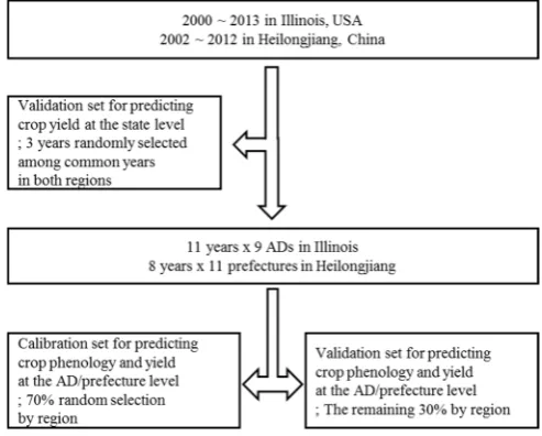
Yield data were classified into two groups for the calibration and validation of phenology and yield. Three years in which yield data were available for both Illinois and Heilongjiang were chosen randomly for validation. Calibration datasets were selected randomly from about 70% of the remaining datasets, including data for the 2000, 2001, and 2013 seasons during which yield data were available in either China or the USA. In total, 69 and 62 sets of yield data were used as the calibration datasets for Illinois and Heilongjiang, respectively (Figure 7). Yield data at the district scale, e.g., AD and prefecture for the USA and China, respectively, were pooled to determine the empirical parameter values, including τ , ρ , α, and β. The other datasets were used to validate the phenology and yield models.
Figure 7. Data-flow diagram showing the process used to classify the calibration and validation datasets.
2.8. Degree of agreement analysis
Degree of agreement statistics were determined by spatial scale, season, and variable. The RMSE value was determined to compare the observed and estimated phenology dates, as follows:
RMSE = 1 ( − ) (10)
where n represents the number of comparisons, and Pi and Oi are the estimated and observed data. Four types of statistics including correlation (R2), normalized root mean square error (NRMSE), the concordance correlation coefficient (CCC), and RMSE were determined for crop yield. The yield of each grid cell was summarized by individual season and district, e.g., AD and prefecture to compare with the reported yields at a regional scale. Yields by region were also aggregated to compare between predicted and reported yields at the state scale, e.g., Illinois and Heilongjiang, by season. The NRMSE was determined as follows [38]:
NRMSE = RMSE ×100
M (11)
where M indicates mean yield reported by the statistical agencies in China and the USA. The simulated results were considered to be either excellent (NRMSE < 10%), good (10% < NRMSE < 20%), fair (20% < NRMSE < 30%), or poor (NRMSE > 30%). The CCC value, which was used to represent precision and accuracy, was determined as follows [39]:
CCC = 2
+ + ( − ) (12)
where ρ is the correlation coefficient between the estimated and reported data, and σ and μ indicate the standard deviations and means of the estimated and observed data, respectively. CCC values closer to unity are better predictors.
3. Results
3.1. Calibration model to predict crop phenology and yield 3.1.1. Crop phenology
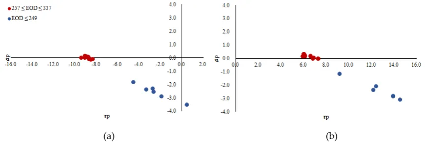
The τ and ρ values differed by the last date on which the remote sensing product was used (EOD) (Figure 8). The τ and ρ values tended to group together by EOD. For example, the τ and ρ values for the emergence and maturity dates were similar after EOD 257.
(a) (b)
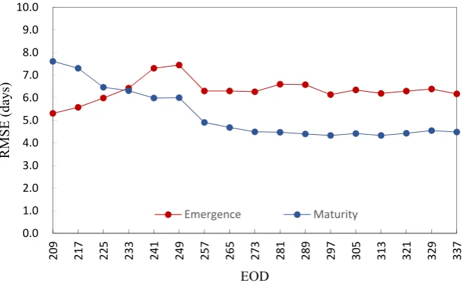
RMSE values for the occurrence date of a phenological stage differed by stage (Figure 9). For example, the RMSE values for maturity (<7 days) were relatively higher than those for emergence (<5 days). Temporal changes in the RMSE value differed by phenological stage. Although the RMSE values decreased with increasing EOD until EOD 257, the error values after EOD 257 were relatively similar.
Figure 9. RMSE values by EOD for the phenology model estimates using a logistic function and the calibration datasets.
3.1.2. Crop yield
The α and β values differed in the YP model and EOD (Figure 10). The α and β values of the YP model grouped together after EOD 257 because they depended on an estimated date for a phenological event, e.g., emergence or maturity. The α and βvalues changed over the EODs when the YF model based on fixed dates was used.
(a) (b)
Figure 10. Estimated α and β values for the YP (a) and YF (b) corn yield models. The X-axis denotes the α values and the Y-axis denotes theβ values.
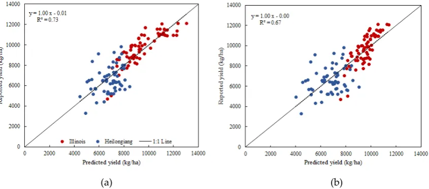
The YP model had a greater degree of agreement for predicting crop yield than the YF model (Figure 11). The R2 values for all EODs of the YP model were higher than those for the YF model when predicting crop yield by district. Although both models predicted differences in crop yield between Illinois and Heilongjiang, the YP model was more precise than the YF model (Figure 12).
0.0 1.0 2.0 3.0 4.0 5.0 6.0 7.0 8.0 9.0 10.0
209 217 225 233 241 249 257 265 273 281 289 297 305 313 321 329 337
RMSE (d
ays)
EOD
Figure 11. R2 values by EOD for the corn yield predictive models by district.
(a) (b)
Figure 12. Comparison between reported and predicted corn yields by district at EOD 257 by the YP (a) and YF (b) models in Illinois and Heilongjiang.
3.2. Validation of the models used to predict crop phenology and yield
The crop phenology and yield prediction models were validated for EODs 209, 257, and 321. The corn silking stage date usually occurs about DOY 209 in Illinois, and the corn harvest was completed near DOY 321. DOY 257 was selected to examine the reliability of the yield predictions in advance because the date was one of the earliest EODs on which maturity dates for corn were reliably predicted in the calibration dataset.
3.2.1. Crop phenology
Figure 13. Comparison between NASS-derived and estimated phenological stages at EOD 257.
The degree of agreement tended to be higher for the estimates of the timing of maturity than those of emergence (Table 1). For example, the RMSE values for maturity were lower than those for emergence. Temporal changes in the degree of agreement statistic also differed.
Table 1. Statistical indices for the phenological stage estimate model in the validation dataset.
EOD Emergence Maturity
R2 RMSE NRMSE R2 RMSE NRMSE
209 0.51 5.31 3.98 0.27 7.61 2.95
257 0.41 6.30 4.72 0.70 4.91 1.90
321 0.35 6.29 4.72 0.78 4.43 1.71
3.2.2. Crop yield by district
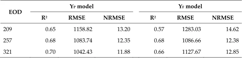
The YP model based on the phenology dates identified from the logistic function had a lower error than that of the YF model based on fixed dates (Table 2). The YP and YF models predicted differences in yield between the two regions, and corn yield was considerably lower in Heilongjiang than in Illinois. Although the YP and YF models for EOD 257 had similar R2 values, the YP model had greater R2 values than those of the YF model for EODs 209 and 321. The YF model always had a higher RMSE than the YP model.
Table 2. Statistical indices for the corn yield prediction models by district.
EOD Y
P model YF model
R2 RMSE NRMSE R2 RMSE NRMSE
209 0.65 1158.82 13.20 0.57 1283.03 14.62
257 0.68 1083.74 12.35 0.68 1086.66 12.38
321 0.70 1042.43 11.88 0.66 1127.67 12.85
100 150 200 250 300
100 150 200 250 300
NASS-der
ived
DOY
Estimated DOY
The errors in yield prediction were similar between EODs 257 and 321 in the YP model. The NRMSE of the crop yield prediction on EOD 257 was slightly greater than that on EOD 321. On the other hand, the YF model had the lowest error on EOD 257.
3.2.3. Crop yield by state
The statistical indices for the corn yield prediction model over 3 years (2003, 2009, and 2012), which were randomly selected, are shown in Table 3. The degree of agreement statistics for the YP model were high for predicting corn yield in Illinois and Heilongjiang. In particular, the YP model performed the best in Illinois, while the YF model had a similar performance in both regions. The R2 and CCC values of both prediction models and regions, except for EOD 209, were > 0.87 and 0.68, respectively. The NRMSE values were 7.39–13.59. Both prediction models and regions exhibited a good performance in predicting corn yield.
Table 3. Statistical indices for the yield prediction models by state in Illinois and by province in Heilongjiang.
Region EOD YP model YF model
R2 RMSE NRMSE CCC R2 RMSE NRMSE CCC
IL
209 0.43 1785.62 19.27 0.21 0.18 2137.85 23.07 -0.12
257 0.87 687.68 7.42 0.93 0.99 1006.67 10.86 0.78
321 0.95 684.72 7.39 0.91 0.94 1068.36 11.53 0.74
HE
209 0.99 1115.68 15.72 0.59 0.96 1008.13 14.20 0.68
257 0.99 964.88 13.59 0.68 0.99 839.75 11.83 0.79
321 0.99 664.07 9.36 0.87 0.99 816.82 11.51 0.79
*IL: Illinois, HE: Heilongjiang
The reported and predicted corn yields by state/province for the prediction models at EOD 257 in Illinois and Heilongjiang are compared in Figure 14.
(a) (b)
4. Discussion
New and simple models were developed to predict corn phenological stages and yield using only red and NIR band surface reflectance data of MODIS products. Sakamoto et al. [40] suggested that the temporal discontinuity of remote sensing data makes it difficult to estimate crop properties, e.g., phenological dates, and therefore different approaches have been developed. Martinez and Gilabert [41] estimated the phenology of the vegetation characterizing a NDVI time series based on wavelet decomposition. In this study, the combination of Equations (4) and (6) allowed us to overcome data discontinuity to estimate the phenological date. The remote sensing data revealed fluctuations in LAI during a season, as shown in Figure 6. However, the integrative approach using Equation (4) made it possible to identify the date of maximum LAI accurately when the EOD was later than 249. Degree of agreement between the observed and predictedphenological stages would increase when the EOD after the maximum LAI was used. For example, a reliable value of b2 was obtained using remote sensing data after the flowering period until near harvest. Because the τ and ρ values depend on b2, long-term data were used to represent growth conditions and obtain reliable estimates of τ and ρ .
The logistic model provided reliable maturity date estimates compared with those of previous studies. Sakamoto et al. [42] reported that the RMSE value of the maturity date for corn in Illinois was 5.9 using the two-step filtering method and WDRVI derived from the MODIS data. The RMSE value of the maturity date on EOD 257 was about 17% less than the previous result when the logistic model was used. In contrast, the logistic model resulted in a greater estimating error for the emergence date. For example, the RMSE value of the emergence date estimated on EOD 257 was 6.3, whereas the value in a previous study was 4.9.
Maturity date depends on the characteristics of the cultivar, such as the physiological response to environmental conditions, and corn phenology is affected by temperature [43]. However, changes in phenology are closely related to changes in LAI. For example, flowering occurs near the time of maximum LAI, which is the b2 value in Equation (4). Once the time of maximum LAI is estimated accurately, the maturity date can be reliably identified. Estimating the maximum LAI using remote sensing products is more accurate than measuring the LAI early in the season when LAI is < 1 [44]. As a result, the accuracy of the maturity date estimate was better than that of the emergence date. Similarly, the accuracy of the maturity date estimate increased when the EOD was late enough to obtain reliable estimates of maximum LAI.
It appeared that errors in the predicted date of emergence were associated with differences in planting dates for a given season in the region of interest. Planting date is influenced by soil temperature and soil moisture and varies widely by district and season (see Appendix A). For example, 33.6 °C is the optimal soil temperature for corn germination [45]. Thus, the planting date would be delayed until that condition is met in a specific field [46,47], which would result in a large variability in the length of the effective growing season in a particular region. The logistic function used in the YP model had relatively low sensitivity for an increase in LAI early in the season, which would result in a relatively large error when estimating the emergence date.
The α and β values for the YP model depended on the reliability of the b3 value, which represents the maximum cumulative LAI. When the EOD before the maximum LAI was used, the b3 value was less reliable because the maximum LAI had not been reached in the field; thus, data up to a specific period after maximum LAI are essential to reliably predict the b3 value. Due to errors in remote sensing data, e.g., caused by clouds and rainfall, maximum LAI estimates can have considerable errors, even after the maximum LAI. Nevertheless, the α and β values were similar after a set of EOD, suggesting that a small range of α and β values could be obtained to predict corn yield.
needed when interpreting differences in RMSE values between current and previous studies. Nevertheless, the RMSE of the YP model tended to be smaller than that of previous studies, which merits further validation in a variety of different regions of interest.
The errors in the YP model for predicting corn yield were also relatively small at the state level. The RMSE values of the YP model were 0.69 t/ha and 0.96 t/ha for Illinois and Heilongjiang, respectively. In previous studies, the RMSE values for predicting corn yield were 0.62–1.45 t/ha in major USA production regions [27, 35]. Sakamoto et al. [21] reported that the RMSE of the corn yield prediction was 0.83 t/ha in Illinois. Nevertheless, their results were obtained from a relatively large number of study regions. Thus, further studies to assess the reliability of the YP model using different approaches would be useful, e.g., WDRVI in other production areas, such as the Midwestern United States. In YP model using only LAI, errors in predicted yield would result from the changes in specific leaf area (SLA) in a given season and region. The SLA is the ratio of leaf area to leaf biomass [50] and is affected by environmental conditions [51], such as weather and disease [52]. As a result, the SLA value differs by season even when the same crops are cultivated at a given site [7]. Because remote sensing products represent LAI instead of biomass, the change in SLA affects the accuracy of estimating biomass and yield using LAI.
5. Conclusions
We developed a new and simple approach to predict corn phenological stages and yields from a minimum MODIS product dataset. Only the surface reflectance red and NIR band data were used to estimate the LAI. Rather than filtering and/or smoothing the LAI data, we fitted the LAI data summed over a cropping season (LAD) to a logistic function. A phenology model was established, with logistic function parameters, and was used to predict emergence and maturity dates within a reasonable range of error. We also developed a simple yield prediction model using LAD over the predicted period from emergence to maturity as a predictor variable. This simple model was also used to predict yields for the two regions selected in this study with considerable precision and accuracy, and could be applied from a fairly early stage of EOD 257. However, these models need to be examined for spatial portability in more diverse agroclimatic regions.
Acknowledgements: This study was conducted with the support of the Cooperative Research Program for Agriculture Science & Technology Development (Project no. PJ0101072016), Rural Development Administration, Republic of Korea.
Author Contributions: Ho-Young Ban and Byun-Woo Lee contributed to the concept design and development of the research; Ho-Young Ban wrote the main manuscript text and prepared the figures and tables, and performed data processing; Ho-Young Ban, Byun-Woo Lee, and Kwang Soo Kim performed data analysis. No-Wook Park collected data of remote sensing; Byun-Woo Lee and Kwang Soo Kim contributed to manuscript improvements.
Conflicts of Interest: The authors declare no conflict of interest.
Appendix A
Figure A1. CV values for the NASS-derived phenological stages in the validation dataset.
References
1. Hayes, M.J.; Decker, W.L. Using NOAA AVHRR data to estimate maize production in the United States Corn Belt. Int. J. Remote Sens.1996, 17, 3189–3200, http://dx.doi.org/10.1080/01431169608949138.
2. Hutchinson, C.F. Uses of satellite data for famine early warning in sub-Saharan Africa. Int. J. Remote Sens.
1991, 12, 1405–1421, http://dx.doi.org/10.1080/01431169108929733.
3. Kouadio, L.; Duveiller, G.; Djaby, B.; Jarroudi, M.E.; Defourny, P. Estimating regional wheat yield from the shape of decreasing curves of green area index temporal profiles retrieved from MODIS data. Int. J. Appl. Earth Obs. Geoinf.2012, 18, 111-118, http://dx.doi.org/10.1016/j.jag.2012.01.009.
4. Macdonald, R.B.; Hall, F.G. Global crop forecasting. Science 1980, 208, 670–679,
http://dx.doi.org/10.1126/science.208.4445.670.
5. Enenkel, M.; Steiner, C.; Mistelbauer, T.; Dorigo, W.; Wagner, W.; See, L.; Atzberger, C.; Schneider, S.; Rogenhofer, E.A. Combined satellite-derived drought indicator to support humanitarian aid organizations. Remote Sens.2016, 8, 340, http://dx.doi.org/10.3390/rs8040340.
6. Casanova, D.; Epema, G.F.; Goudriaan, J. Monitoring rice reflectance at field level for estimating biomass and LAI. Field Crops Res.1997, 55, 83-92, http://dx.doi.org/10.1016/s0378-4290(97)00064-6.
7. Maki, M.; Homma, K. Empirical Regression Models for Estimating Multiyear Leaf Area Index of Rice from Several Vegetation Indices at the Field Scale. Remote Sens. 2014, 6, 4764-4779,
http://dx.doi.org/10.3390/rs6064764.
8. Liu, X.; Jin, J.; Herbert, S.J.; Zhang, Q.; Wang, G. Yield components, dry matter, LAI and LAD of soybeans in Northeast China. Field Crops Res.2005, 93, 85-93, http://dx.doi.org/10.1016/j.fcr.2004.09.005.
9. López-Bellido, F.J.; López-Bellido, R.J.; Khalil, S.K.; López-Bellido, L. Effect of Planting Date on Winter Kabuli Chickpea Growth and Yield under Rainfed Mediterranean Conditions. Agron. J.2008, 4, 957-964,
http://dx.doi.org/10.2134/agronj2007.0274.
10. Huang, J.; Wang, X.; Li, X.; Tian, H.; Pan, Z. Remotely sensed rice yield prediction using multi-temporal
NDVI data derived from NOAA’s-AVHRR. PLoS ONE 2013, 8, e70816,
http://dx.doi.org/10.1371/journal.pone.0070816.
11. Wang, Q.; Adiku, S.; Tenhunen, J.; Granier, A. On the relationship of NDVI with leaf area index in a deciduous forest site. Remote Sens. Environ.2005, 94, 244-255, http://dx.doi.org/10.1016/j.rse.2004.10.006. 12. Ochi, S.; Shibasaki, R.; Murai, S. Modeling and assessment of NPP/crop productivity in Asia by GIS
combined with remote sensing data. International Rice Research Institute (IRRI) Los Banos, Philippines, 2–3 November 2000.
13. Rossini, M.; Cogliati, S.; Meroni, M.; Migliavacca, M.; Galvagno, M.; Busetto, L.; Cremonese, E.; Julitta, T.; Siniscalco, C.; Morra di Cella, U.; Colombo, R. Remote sensing-based estimation of gross primary production in a subalpine grassland. Biogeosciences 2012, 9, 2565-2584,
http://dx.doi.org/10.5194/bgd-9-1711-2012.
14. Wiegand, C.L.; Richardson, A.J. Leaf area, light interception, and yield estimates from spectral components analysis. Agron. J.1984, 76, 543-548, http://dx.doi.org/10.2134/agronj1984.00021962007600040008x.
15. Kussul, N.; Shelestov, A.; Skakun, S. Grid and sensor web technologies for environmental monitoring. Earth Sci. Inform.2009, 2, 37–51, http://dx.doi.org/10.1007/s12145-009-0024-9.
6.81
5.49
2.27 3.03
0.0 2.0 4.0 6.0 8.0 10.0
Planting Emergence Silking Maturity
16. Jaafar, H.H.; Ahmad, F.A. Crop yield prediction from remotely sensed vegetation indices and primary productivity in arid and semi-arid lands. Int. J. Remote Sens. 2015, 36, 4570-4589,
http://dx.doi.org/10.1080/01431161.2015.1084434.
17. Kolotii, A.; Kussul, N.; Shelestov, A.; Skakun, S.; Yailymov, B.; Basarab, R.; Lavreniuk, M.; Oliinyk, T.; Ostapenko, V. Comparison of biophysical and satellite predictors for wheat yield forecasting in Ukraine. Int. Arch. Photogramm. Remote Sens. 2015, XL-7/W3, 39-44,
http://dx.doi.org/10.5194/isprsarchives-xl-7-w3-39-2015.
18. Rembold, F.; Atzberger, C.; Savin, I.; Rojas, O. Using low resolution satellite imagery for yield prediction and yield anomaly detection. Remote Sens.2013, 5, 1704-1733, http://dx.doi.org/10.3390/rs5041704.
19. Sibley, A.M.; Grassini, P.; Thomas, N.E.; Cassman, K.G.; Lobell, D.B. Testing remote sensing approaches for assessing yield variability among maize fields. Agron. J. 2014, 106, 24-32,
http://dx.doi.org/10.2134/agronj2013.0314.
20. Islam, A.S.; Bala, S.K. Assessment of Potato Phenological Characteristics Using MODIS-Derived NDVI and LAI Information. Gisci. Remote Sens.2008, 45, 454-470, http://dx.doi.org/10.2747/1548-1603.45.4.454.
21. Sakamoto, T.; Gitelson, A.A.; Arkebauer, T.J. MODIS-based corn grain yield estimation model incorporating crop phenology information. Remote Sens. Environ. 2013, 131, 215-231,
http://dx.doi.org/10.1016/j.rse.2012.12.017.
22. Vina, A.; Gitelson, A.A.; Rundquist, D.C.; Keydan, G.; Leavitt, B.; Schepers, J. Monitoring maize (Zea mays L.) phenology with remote sensing. Agron. J.2004, 96, 1139-1147, http://dx.doi.org/10.2134/agronj2004.1139. 23. Prasad, P.V.V.; Staggenborg, S.A.; Ristic, Z. Impacts of drought and/or heat stress on physiological,
developmental, growth, and yield processes of crop plants. In Response of Crops to Limited Water: Understanding and Modeling Water Stress Effects on Plant Growth Processes; Ahuja, L.H., Saseendran, S.A., Eds.; Advances in Agricultural Systems Modeling Series 1. ASA-CSSA: Madison, WI, USA, 2008; pp. 301–355,
http://dx.doi.org/10.2134/advagricsystmodel1.c11.
24. Li, A.; Liang, S.; Wang, A.; Qin, J. Estimating crop yield from multi-temporal satellite data using multivariate regression and neural network techniques. Photogramm. Eng. Rem. S. 2007, 73, 1149-1157,
http://dx.doi.org/10.14358/pers.73.10.1149.
25. Huang, L.; Yang, Q.; Liang, D.; Dong, Y.; Xu, X.; Huang, W. The estimation of winter wheat yield based on MODIS remote sensing data. Computer and Computing Technologies in Agriculture V. IFIP Advances in Information and Communication Technology, Springer, October, Berlin Heidelberg 2011, pp. 496-503,
http://dx.doi.org/10.1007/978-3-642-27278-3_51.
26. Lobell, D.B. The use of satellite data for crop yield gap analysis. Field Crops Res. 2013, 143, 56-64,
http://dx.doi.org/10.1016/j.fcr.2012.08.008.
27. Prasad, A.K.; Chai, L.; Singh, R.P.; Kafatos, M. Crop yield estimation model for Iowa using remote sensing and surface parameters. Int. J. Appl. Earth Obs. Geoinf. 2006, 8, 26-33,
http://dx.doi.org/10.1016/j.jag.2005.06.002.
28. Zhang, H.; Chen, H.; Zhou, G. The Model of Wheat Yield Forecast based on MODIS-NDVI: A Case Study of XinXiang. ISPRS Annals of the Photogrammetry, Remote Sensing and Spatial Information Sci., I-7, XXII ISPRS Congress. Melbourne, Australia, 25 August – 01 September 2012,
http://dx.doi.org/10.5194/isprsannals-i-7-25-2012.
29. Eberhart, S.T.; Russell, W.A. Stability parameters for comparing varieties. Crop Sci. 1966, 6, 36-40,
http://dx.doi.org/10.2135/cropsci1966.0011183x000600010011x.
30. Kim, Y.; Lee, K.D.; Na, S.I.; Hong, S.Y.; Park, N.W.; Yoo, H.Y. MODIS data-based crop classification using selective hierarchical classification. Korean J. Remote Sens. 2016, 32, 235-244,
http://dx.doi.org/10.7780/kjrs.2016.32.3.3.
31. Nguy-Robertson, A.L.; Gitelson, A.A.; Peng, Y.; Viña, A.; Arkebauer, T.J.; Rundquist, D.C. Green Leaf Area Index Estimation in Maize and Soybean: Combining Vegetation Indices to Achieve Maximal Sensitivity. Agron. J.2012, 104, 1336-1347, http://dx.doi.org/10.2134/agronj2012.0065.
32. Rouse, J.; Hass, R.; Schell, J.; Deering, D. Monitoring vegetation systems in the great plains with ERTS. In
Third ERTS Symposium; 1973; NASA: SP-351 I; pp. 309–317.
33. Jordan, C.F. Derivation of leaf-area index from quality of light on the forest floor. Ecology1969, 50, 663-666,
http://dx.doi.org/10.2307/1936256.
35. Shao, Y.; Campbell, J.B.; Taff, G.N.; Zheng, B. An analysis of cropland mask choice and ancillary data for annual corn yield forecasting using MODIS data. Int. J. Appl. Earth Obs. Geoinf. 2015, 38, 78-87,
http://dx.doi.org/10.1016/j.jag.2014.12.017.
36. Nelder, J.A.; Mead, R. A simplex method for function minimization. The Computer J. 1965, 7, 308-313,
http://dx.doi.org/10.1093/comjnl/7.4.308.
37. Power, J.F.; Willis, W.O.; Reichman, G.A. Effect of soil temperature, phosphorus and plant age on growth analysis of barley. Agron. J.1967, 59, 231-234, http://dx.doi.org/10.2134/agronj1967.00021962005900030007x. 38. Soler, C.; Sentelhas, P.; Hoogenboom, G. Application of the CSM-CERES-Maize model for planting date
evaluation and yield forecasting for maize grown off-season in a subtropical environment. Eur. J. Agron.
2007, 27, 165-177, http://dx.doi.org/10.1016/j.eja.2007.03.002.
39. Lin, L. A concordance correlation coefficient to evaluate reproducibility. Biometrics. 1989, 45, 255–268,
http://dx.doi.org/10.2307/2532051.
40. Sakamoto, T.; Yokozawa, M.; Toritani, H.; Shibayama, M.; Ishitsuka, N.; Ohno, H. A crop phenology detection method using time-series MODIS data. Remote Sens. Environ. 2005, 96, 366-374,
http://dx.doi.org/10.1016/j.rse.2005.03.008.
41. Martinez, B.; Gilabert, M.A. Vegetation dynamics from NDVI time series analysis using the wavelet transform. Remote Sens. Environ.2009, 113, 1823–1842, http://dx.doi.org/10.1016/j.rse.2009.04.016.
42. Sakamoto, T.; Wardlow, B.D.; Gitelson, A.A. Detecting spatiotemporal changes of corn developmental stages in the U.S. corn belt using MODIS WDRVI data. IEEE Trans. Geosci. Remote Sens.2011, 49, 1926-1936,
http://dx.doi.org/10.1109/tgrs.2010.2095462.
43. Cutforth, H.W.; Shaykewich, C.F. A temperature response function for corn development. Agr. Forest Meteorol.1990, 50, 159-171, http://dx.doi.org/10.1016/0168-1923(90)90051-7.
44. Heiskanen, J.; Rautiainen, M.; Stenberg, P.; Mõttus, M.; Vesanto, V. H.; Korhonen, L.; Majasalmi, T. Seasonal variation in MODIS LAI for a boreal forest area in Finland. Remote Sens. Environ. 2012, 126, 104-115,
http://dx.doi.org/10.1016/j.rse.2012.08.001.
45. Itabari, J.K.; Gregory, P.J.; Jones, R.K. Effects of temperature soil water status and depth of planting on germination and emergence of maize (Zea mays) adapted to semi-arid eastern Kenya. Expl. Agric.1993, 29, 351-364, http://dx.doi.org/10.1017/s0014479700020913.
46. Chen, G.H.; Wiatrak, P. Soybean development and yield are influenced by planting date and environmental conditions in the southeastern coastal plain, United States. Agron. J. 2010, 102, 1731-1737,
http://dx.doi.org/10.2134/agronj2010.0219.
47. Thomison, P.; Nielson, R. Impact of Delayed Planting on Heat Unit Requirements for Seed Maturation in Maize, vol. 15. Pontificia Universidad Católica deChile. Departamento de Ciencias Vegetales. Seminario Internacional Semillas:comercialización producción y tecnología, Santiago, 2002, pp. 140–164.
48. Doraiswamy, P.C.; Akhmedov, B.; Beard, L.; Stern, A.; Mueller, R. Operational prediction of crop yields using MODIS data and products. International archives of photogrammetry, remote sensing and spatial information, Sciences Special Publications, Commission Working Group VIII WG VIII/10. Ispra, Italy: European Commission DG JRC-Institute for the Protection and Security of the Citizen, 2007, 1-5.
49. Johnson, D.M. An assessment of pre-and within-season remotely sensed variables for forecasting corn and soybean yields in the United States. Remote Sens. Environ. 2014, 141, 116-128,
http://dx.doi.org/10.1016/j.rse.2013.10.027.
50. Setiyono, T.D.; Weiss, A.; Specht, J.E.; Cassman, K.G.; Dobermann, A. Leaf area index simulation in soybean grown under near-optimal conditions. Field Crops Res. 2008, 108, 82–92,
http://dx.doi.org/10.1016/j.fcr.2008.03.005.
51. Gunn, S.; Farrar, J.F.; Collis, B.E.; Nason, M. Specific leaf weight in barley: individual leaves versus whole plants. New Phytol. 1999, 413, 45–51, http://dx.doi.org/10.1046/j.1469-8137.1999.00434.x.
52. Kim S.H.; Hong S.Y.; Sudduth K.A.; Kim Y.; Lee K. Comparing LAI estimates of corn and soybean from vegetation indices of multi-resolution satellite images. Korean J. Remote Sens. 2012, 28, 597–609,
http://dx.doi.org/10.7780/kjrs.2012.28.6.1.