Forestry & Natural-Resource Sciences Last Correction: Mar. 8, 2013
INFLUENCE OF THE JUXTAPOSITION OF TREES ON
CONSUMER-GRADE GPS POSITION QUALITY
Pete Bettinger
1, Krista L. Merry
21Professor,2Res. Coordinator. Warnell School of Forestry & Natural Resources, University of Georgia, Athens, GA, USA
Abstract. Until now, limited observational data have suggested that the juxtaposition of trees with
respect to place where a GPS position fix is collected may affect static horizontal position accuracy of that determined position. Our goal was to assess GPS accuracy with respect to the spatial arrangement of nearby trees, and determine whether correlations existed or whether trends were evident. Therefore, static horizontal position accuracy of a consumer-grade GPS receiver was estimated in a young loblolly pine (Pinus taeda) plantation in Georgia (USA) to determine whether the arrangement of trees had any influence on position quality. Thirty visits to twenty-nine test points, randomly ordered, were made to collect the necessary data regarding positional accuracy. No significant relationship was observed between static horizontal positional accuracy and environmental variables (air temperature, relative humidity, and atmospheric pressure) or the planned positional dilution of precision (PDOP) of the NAVSTAR satellite configuration. However, we found moderate correlation between average positional error and a few forest structure measures. For example, we observed that as hardwood (deciduous species) basal area and hardwood tree count within 4 or 5 m of a test point increased, the average positional error tended to increase. No significant correlation was observed using forest structure values obtained within 3 m of each test point. Using rose diagrams (circular histograms), we observed that in some cases there seemed to be a negative attraction between the location of live trees and the position determined by the GPS receiver. Using vectors to represent magnitude and direction of both GPS error and forest conditions, we found evidence to conclude that the average distance and direction to live deciduous (hardwood) trees within this young pine forest may have some influence on position quality.
Keywords: Global positioning systems, GNSS, root mean squared error, static horizontal position accuracy, rose diagram, circular histogram
1
Introduction
Global navigation satellite systems (GNSS) have be-come a pervasive technology in natural resource man-agement and in environmental research studies. Satel-lite positioning systems are typically referred to asGPS (Global Positioning Systems) in North America. They are based on electromagnetic energy emitted by satel-lites situated (or orbiting) several thousand kilometers above the landscape, and received by devices on Earth in order to determine a position (Bettinger and Merry 2011). While the Russian Federation has a satellite nav-igation system (GLONASS) that is currently used inter-nationally, and while the European Union and China are currently developing global satellite navigation systems (GALILEO and COMPASS), this study focuses on po-sitions determined using the United States NAVSTAR system. The NAVSTAR system consists of 31 satellites,
allocated to one of six orbital planes around the Earth. Each satellite broadcasts a unique signal on the L1 fre-quency (1575.42 MHz) using coarse acquisition (C/A) code. Commercially available GPS receivers can utilize this code to determine both horizontal and vertical po-sitions on the Earth.
GPS receivers are generally classified as survey-grade, mapping-survey-grade, or recreation-grade (or consumer-grade), based primarily on cost and subsequently on the technology available in each. Recreation-grade GPS re-ceivers vary in price from $100 to $600, and provide the least accurate static horizontal positions, generally accompanied with 5-15 m of error (Wing et al. 2005, Danskin et al. 2009b). Most natural resource manage-ment organizations use mapping-grade receivers, which range in price from about $1,000 to $8,000, and can now determine static positions within about 2 m of true
sitions (Ransom et al. 2010). Survey-grade GPS re-ceivers can provide sub-meter accuracy for static posi-tions in forests, yet these receivers are generally more expensive, bulky, heavy, and may require several min-utes of data collection at each sampling point. In the last few years, GPS technology assessments have mainly concentrated on static horizontal position determination (Anderson et al. 2009, Bakula et al. 2009, Bettinger and Fei 2010, Klim´anek 2010, Pirti et al. 2010, Ransom et al. 2010, Wing 2009), although dynamic assessments (e.g., Tachiki et al. 2005) and assessments of static vertical position accuracy (Bakula et al. 2009, Klim´anek 2010, Pirti et al. 2010) have also been performed and reported. The main conclusions drawn from recent studies on the static horizontal position accuracy of GPS technology used in forested environments are as follows:
1. Some (e.g., Oderwald and Boucher 2003) have sug-gested that under certain conditions differential correc-tion of GPS data may no longer be necessary after the discontinuation of the selective availability process in 2000. Recent tests suggest that differential correction of data collected by a mapping-grade receiver under a forest canopy can improve horizontal position accuracy (Danskin et al. 2009a, 2009b), yet results are not uni-versally conclusive (e.g., Wing et al. 2008).
2. Multipath error in forested conditions can account for over half of the error in static horizontal positions (Danskin et al. 2009a), and the ability of a GPS re-ceiver to reject multipath signals may be the main rea-son why consumer-grade receivers have lower static hor-izontal position accuracy than mapping-grade receivers (Bolstad et al. 2005).
3. Slope position (e.g., upper vs. lower) can be in-fluential on static horizontal position accuracy (Deckert and Bolstad 1996, Danskin et al. 2009a, 2009b), with po-sitions determined on upper slopes having higher static horizontal position accuracy (lower error) than positions determined on lower slopes.
4. The number of position fixes (epochs, or way-points) necessary to effectively determine a static hor-izontal position under a forest canopy is debatable. A decade or more ago it was suggested that perhaps 300 position fixes were necessary (Sigrist et al. 1999). How-ever, recent research suggests that a position determined from a single position fix may generally be no less accu-rate than one determined from an average of a number of position fixes (Bolstad et al. 2005, Wing and Karsky 2006, Bettinger and Merry 2012).
5. Although high-precision GPS applications may be affected by propagation delay due to atmospheric con-ditions (Chen et al. 2008), particularly during the pas-sage of weather fronts (Ghoddousi-Fard et al. 2009), atmospheric conditions have been shown to have little effect on static horizontal accuracy in forested
condi-tions (Bolstad et al. 2005, Bettinger and Fei 2010). In a study of a consumer-grade receiver over the course of one year, Bettinger and Fei (2010) found no significant relationship between static horizontal position accuracy and ionospheric or tropospheric variables (air tempera-ture, relative humidity, atmospheric pressure, and solar wind speed).
6. The type of forest (species or age) under which tests are made can influence the accuracy of static hor-izontal positions (Deckert and Bolstad 1996, Yoshimura and Hasegawa 2003, Wing et al. 2005, Wing and Karsky 2006, Wing et al. 2008, Andersen et al. 2009, Bettinger and Fei 2010).
7. The height of a GPS antenna, when used in forested conditions, can have an effect on static horizon-tal position accuracy (D’Eon 1996, Wing et al. 2008).
8. Canopy closure may have an effect on static hori-zontal position accuracy (Sigrist et al. 1999, Veal et al. 2001). Thus the time of year when data are collected can influence static horizontal position accuracy (Dan-skin et al. 2009b, Bettinger and Fei 2010), particularly when considering deciduous forests.
Although not rigorously tested, the configuration of vegetation (the juxtaposition of trees with respect to place where a position fix is collected) may affect static horizontal position accuracy, and has been suggested by Hasegawa and Yoshimura (2003), Danskin et al. (2009b), Wing (2009), and Bettinger and Fei (2010) as an issue that still needs to be addressed. As a result, the objectives of this work were to understand whether tree position within the immediate area of GPS data col-lection processes has an effect on static horizontal posi-tion accuracy. One hypothesis tested here suggests that static horizontal position accuracy would not change due to tree position or tree density around the position that needed to be determined, given the GPS receiver stud-ied. Other hypotheses we tested, because they were co-incidental to the work and in order to provide further support for the previous conclusions drawn, suggest that static horizontal position accuracy would not change as environmental conditions (air temperature, relative hu-midity, etc.) change.
2
Methods
Using a known location on the GPS Test Site at the Whitehall Forest GPS Test Site in Athens, Geor-gia (USA) as a starting point, 28 test points on a 3 m grid were carefully delineated using a steel tape. This test area is situated within a young loblolly pine (Pinus taeda) plantation (18 years old, unthinned, 41.3 m2 per
hectare accounting for 1.6 m2 per hectare of basal area. A Garmin Oregon 300 consumer-grade GPS receiver was employed in this study because a previous study (Bet-tinger and Fei 2010) noted that the error when using this receiver was biased at the original test point, but not in other nearby study areas.
The 28 temporary test points and original GPS test point were visited 30 times over the course of a month (mid-June to mid-July 2012), and ten position fixes were collected at each test point during each visit. We chose ten position fixes to determine an average point loca-tion because: (a) recent evidence with this exact GPS receiver suggested that the first position fix was not sig-nificantly different than an average of 50 position fixes in most forest types, yet minor differences do occur in young pine forests (Bettinger and Merry 2012), and (b) the time required to collect data on 29 test points was extensive. Therefore, ten position fixes was a compro-mise made in order to capture some of the variation in position determination measurements that will occur. These ten position fixes were averaged to determine the static horizontal position accuracy for each visit to each test point. The order of data collection on each of the 29 test points was randomized for each visit.
In order to ensure consistent parameter settings and environmental variables throughout the study period, near real-time augmentation using the United States Wide Area Augmentation System (WAAS) was disabled. This augmentation service cannot guarantee 100% avail-ability, and the GPS receiver was unable to record when the augmentation system was being used. Position fixes (epochs, or waypoints) were captured manually, with 2-3 second intervals, because the GPS receiver employed does not have the ability to collect data automatically everyxseconds. At the beginning of each visit, a warm-up period was required, and during data collection GPS receiver was plumbed approximately 1 m directly over each of the 29 test points using a staff and a plumb bob. The person collecting the data was positioned consis-tently on the west side of each test point as data was being collected. A concerted effort was made so that the body of the person collecting the data would not in-terfere with the signals. While ideally a person would be situated between the position to be determined and the lowest point on the landscape (maximizing the view above the horizon), the slope in this area was low (8%) and given the arrangement of test points and trees, the best consistent position for the data collector was to stand to the west of each test point.
Weather data (relative humidity, atmospheric pres-sure) for the Athens, Georgia area at the time of each visit was obtained from the Internet site Weather Un-derground (www.wunUn-derground.com). Air temperature measurements were obtained using an on-site
thermome-ter. The planned PDOP (Positional Dilution of Preci-sion) for the data collection periods was acquired using Trimble GPS planning software and a current almanac, since actual PDOP measurements were unavailable from the GPS receiver studied. Although a direct comparison of planned and actual PDOPs has not been conducted, we assume that the planned PDOPs are lower than the actual because planned PDOPs seem to be determined for ideal conditions, while actual PDOPs take into ac-count that some of the ideal satellites are not used to determine a position due to obstructions (trees). The accuracy of static horizontal positions was reported as a root mean squared error (RMSE):
RMSE = n i
(xi−xT)2+ (yi−yT)2
n (1)
Here, n is the total number of observations (position fixes) during a visit to each test point, iis the ith ob-servation during each visit (i = 1 to n). In addition,
xi and yi represent the estimated easting and northing
values of theith observation, respectively, in the UTM, NAD 1983 coordinate system. And,xT andyT represent the true easting and northing values of the test point. These average RMSE values for each visit to each test point were used along with the weather conditions in the statistical analysis.
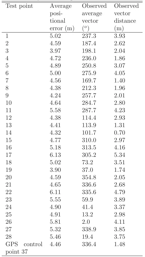
trees were composed mainly of small-diameter sweetgum (Liquidambar styraciflua), although a few black cherry (Prunus serotina), water oak (Quercus nigra) and other minor species were measured. From this information, and using the estimated location of each tree (Figure 1), we developed 50 forest structure variables (Table 1) in preparation for determining whether there was an as-sociation between these and the average static horizon-tal position error observed at each temporary test point. Trees within 5 m of each temporary test point were used to compute the forest structure variables.
Table 1: Forest structure variables used in the analysis of static horizontal position accuracy. These involved mea-surements of live trees, and were summarized as values within 1, 2, 3, 4, and 5 m from each test point.
Total tree count Total tree basal area Pine tree count Pine basal area Hardwood tree count Hardwood basal area
Average departure (east-west orientation) of pine trees from each test point†
Average latitude (east-west orientation) of pine trees from each test point†
Average departure (east-west orientation) of hard-wood trees from each test point†
Average latitude (east-west orientation) of hardwood trees from each test point†
†These distances were weighted by the diameter of each tree,
therefore larger diameter trees had greater influence on these values than smaller diameter trees.
Correlation analyses were performed between the dependent variable values (error) and other variables (PDOP, air temperature, relative humidity, atmospheric pressure, etc.). Pearson’s r correlation coefficient was used to measure correlation among the variables. In this study, we also use correlation analysis to determine the strength to which forest structure variables are associ-ated with average positional error, departure (east-west) error, and latitude (north-south) error. Rose diagrams (circular histograms) were then developed to visually as-sess the association between the direction of error and two of the fifty forest structure values. The magnitude of positional error, expressed as the distance associated with the average departure and latitude, was developed for each of the test points. The average latitude and dis-tance to all trees, pine trees, and hardwood trees within 5 m of each test point was then developed and converted into a vector representing the magnitude of these for-est conditions. These were also then weighted by the
Table 2: Average positional error (RMSE), observed av-erage vector of the error (using avav-erage departure and latitude values), and average vector distance.
Test point Average
posi-tional error (m) Observed average vector (o)
Observed vector distance (m)
1 5.02 237.3 3.93
2 4.59 187.4 2.62
3 3.97 198.1 2.04
4 4.72 236.0 1.86
5 4.89 250.8 3.07
6 5.00 275.9 4.05
7 4.56 169.7 1.40
8 4.38 212.3 1.96
9 4.24 257.7 2.01
10 4.64 284.7 2.80
11 5.58 287.7 4.23
12 4.38 114.4 2.93
13 4.41 113.9 1.31
14 4.32 101.7 0.70
15 4.77 310.0 2.97
16 5.18 313.5 4.16
17 6.13 305.2 5.34
18 5.02 73.2 3.51
19 3.90 37.0 1.74
20 4.59 354.8 2.05
21 4.65 336.6 2.68
22 6.11 335.6 4.79
23 5.55 59.9 3.89
24 4.90 41.4 3.37
25 4.91 13.2 2.98
26 5.81 2.0 4.11
27 5.32 338.9 3.85
28 5.46 19.4 3.75
GPS control point 37
4.46 336.4 1.48
Figure 1: The arrangement of temporary test points, pine trees, and hardwood trees around GPS test point 37 of the Whitehall Forest GPS Test Site.
by azimuth values) were then transformed using the logic below in order to normalize the data:
If (azimuth 180˚), then transformed azimuth = azimuth / 180˚
Else, transformed azimuth = (180˚ (azimuth -180˚)) / 180˚
When applying this transformation, azimuths rep-resenting South (near 180˚) are converted to values around 1.0, while azimuths representing North (near 0˚ or near 360˚) are converted to values around 0.0, regard-less of which side of North the azimuths lie. Correlation analyses using Pearson’s r correlation coefficient were then applied to determine whether any association exists between thedirectionof positional error and the vectors representing the direction forest conditions within 5 m of each test point.
3
Results
Over the entire course of the study, the average posi-tional error for all 29 test points was 4.88 m, yet ranged from 3.90 to 6.13 m depending on the test point (Ta-ble 2). In examining each individual day of the study period, we found that the average error of 10 position fixes ranged from 0.17 to 22.70 m. The average posi-tional error determined for each day, for each test point (from the collection of ten position fixes captured at each test point on each day) was used to determine whether
these were correlated with environmental variables and planned PDOP. Of the environmental variables mea-sured, none had a significant effect on positional error. Mean error values were very weakly positively correlated with relative humidity (0.114) and very weakly nega-tively correlated with air temperature (-0.161). Baro-metric pressure and planned PDOP of the NAVSTAR satellite configuration had even less association with ob-served error in static horizontal positions.
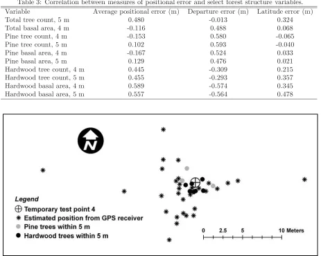
Table 3: Correlation between measures of positional error and select forest structure variables.
Variable Average positional error (m) Departure error (m) Latitude error (m)
Total tree count, 5 m 0.480 -0.013 0.324
Total basal area, 4 m -0.116 0.488 0.068
Pine tree count, 4 m -0.153 0.580 -0.065
Pine tree count, 5 m 0.102 0.593 -0.040
Pine basal area, 4 m -0.167 0.524 0.033
Pine basal area, 5 m 0.129 0.476 0.021
Hardwood tree count, 4 m 0.445 -0.309 0.215
Hardwood tree count, 5 m 0.455 -0.293 0.357
Hardwood basal area, 4 m 0.589 -0.574 0.345
Hardwood basal area, 5 m 0.557 -0.564 0.478
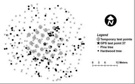
Figure 2: The arrangement of determined positions of temporary test point 4 in relationship with the true position of temporary test point 4 and nearby pine and hardwood trees.
as these structural variables increased in magnitude, av-erage positional error tended to increase, and as they decreased in magnitude, average positional error tended to decrease. Interestingly, the correlation analysis sug-gested that these variables were low to moderately neg-atively correlated with departure error, suggesting that as these structural variables increased in magnitude, de-parture error tended to be toward the west. As they decreased in magnitude, departure error tended to be toward the east. These variables were also low to mod-erately positively correlated with latitude error, suggest-ing that as these structural variables increased in mag-nitude, departure error tended to be toward the north. As they decreased in magnitude, latitude error tended to be toward the south. Pine tree count and pine basal area (both 4 m and 5 m distances), along with total tree basal area within 4 m of a test point, were mod-erately positively correlated with departure (east-west)
error. This suggests that as these structural variables increased in magnitude, departure error tended to be toward the east.
direction of error. For example, assume two samples produced RMSE values of 4.0 m and 3.0 m. The aver-age positional error of these is 3.5 m. However, if one of these was oriented to the north of a sample point, and one was oriented to the south, the observed vector dis-tance would be 0.5 m, and would also be oriented to the north.
To further illustrate some of the issues concerning the orientation of error and the orientation of forest condi-tions, Figure 3 provides a glimpse of four of the test points, their average error, and total tree count and hardwood tree count within 5 m of each test point. For example, results from test point 8 suggest that the static horizontal error from 30 visits was concentrated to the south of the test point (Figure 3, part a). Interestingly, live trees were concentrated to the northwest and north-east of the test point (Figure 3, parts b and c). Results from test point 12 suggest that static horizontal error was concentrated to the southeast of the test point (Fig-ure 3, part d), while live trees were concentrated to the northeast of the test point (Figure 3, parts e and f). In-terestingly, results from test point 22 suggest that static horizontal error was concentrated to the northwest of the test point (Figure 3, part g), while live trees were perhaps more concentrated to the south of the test point (Figure 3, part h). Similarly, results from test point 24 suggest that static horizontal error was concentrated to the northeast of the test point (Figure 3, part j), while live trees were perhaps more concentrated to the south of the test point (Figure 3, parts k and l). These results seem to indicate a trend where the determined position from the GPS receiver was negatively attracted to the location of the trees within 5 m of each test point. How-ever, there are many combinations of forest parameters that might be explored to further elucidate these trends, and the trends were not entirely evident in some cases. Admittedly, more effort can be extended to an explo-ration of these relationships using methods described by Jones (2006a, 2006b) and others. We leave this as an open area of research for others to pursue since some of the directional analysis concepts described in previous work have not yet been applied to the type of forestry data provided here.
In examining the magnitude of error observed in con-junction with the average distance to trees around each test point (Table 4), we found significant negative cor-relation with the number of hardwood trees and with the basal area of hardwood trees. This suggests that GPS error decreased as the average distance (simple av-erage or weighted by basal area) increased from each test point, regardless of the orientation of these trees with respect to the test point. When the direction of average GPS error was compared to the average direc-tion to the trees around each test point, a weak negative
correlation (-0.345) between the average vector repre-senting the direction to hardwood trees and the average direction of GPS error was observed. These results lend credence to the notion that the error observed with the GPS receiver tested may be influenced by the number and orientation of hardwood trees within a young pine stand that are situated around a test point where static horizontal positions are collected.
Table 4: Correlation (Pearson’s r) between measures of direction (azimuth) and magnitude (meters) of po-sitional error and direction (azimuth) and magnitude (meters) of tree locations.
Variable Plot
Radius (m)
Average magnitude of error
Average direction of error
Total tree count 5 -0.283 -0.167
Total basal area 5 0.261 0.015
Pine tree count 5 -0.065 0.229
Pine basal area 5 0.259 0.014
Hardwood tree count 5 -0.557† -0.345
Hardwood basal area 5 -0.430† -0.072
†p <0.05 ; ‡p <0.01
4
Discussion
When employing a recreation-grade GPS receiver in a dense young pine forest in the southern United States, we found that most forest structure variables were weakly correlated (0.400 to -0.400) with the three mea-sures of error (average straight-line error [RMSE]), av-erage departure error [east-west], and avav-erage latitude error [north-south]). In fact, the highest correlation val-ues were found for forest structure variables within 4 or 5 m of each test point, rather than 1-3 m. This is perhaps because while some vegetation was situated within 1-3 m of a test point, more vegetation was situated within 4-5 m. It should be noted, that the test point locations were not affected (nor adjusted) as a result of the vegetation found in the sample area. One test point was in fact mere centimeters from two different trees, and others were situated near or within clumps of small hardwood trees.
static horizontal position accuracy may be necessary to determine more precisely the causes of error. These in-clude exploration of the correlation between two vari-ables that are described in a circular manner. Figure 3 illustrated this data graphically using a rose diagram, which was essentially a frequency distribution of error vectors and tree locations in 30o increments. The asso-ciation between these types of data could employ canon-ical correlation coefficients, T-monotone or T-linear as-sociations, resampling, and a deconstruction of the az-imuthal variable into components such as the departure and latitudes described here. However, these analyses are beyond the scope of this exploratory study and left for others to pursue.
As with recent studies of GPS receivers in forested settings (Bettinger and Fei 2010, Ransom et al. 2010), in this study there was very little association between static horizontal position accuracy, environmental vari-ables, and planned PDOP. It therefore seems safe to say that lower atmospheric conditions that are typically measured (air temperature, relative humidity, baromet-ric pressure) have little effect on some consumer-grade receiver accuracy in forested conditions, at least within typical ranges of values observed in the southern United States. From the analyses provided here is also seems safe to say that within young pine forests, the density and distribution of hardwood volunteers may affect the quality of GPS data collected. However, in studies such as these, where control over data methods is necessary, the full range of potential factors influencing data qual-ity have not been addressed. Therefore, the position of the data collector with respect to test points, and the use of near-real time augmentation (i.e., WAAS) may need further exploration.
5
Conclusions
We hypothesized that static horizontal position accu-racy of a consumer-grade GPS receiver would not be influenced by environmental conditions or satellite ge-ometry, and as in previous studies, we found that we could not reject this hypothesis. However, we found ev-idence to conclude that the density and arrangement of live deciduous (hardwood) trees within a young pine forest may have some influence on position quality. Our results also indicate that there was a moderate correla-tion between average static horizontal posicorrela-tion error and a few measures of forest structure within 5 m of a sam-pling point. As suggested, within a young pine forest, hardwood basal area and hardwood tree count seemed to be the most important of these variables. Interest-ingly, forest vegetation closer than 4 m from a test point did not seem to influence static horizontal position ac-curacy. Further, using rose diagrams that illustrate the
direction of error and the direction of forest vegetation with respect to the location of a test point, we observed some negative attraction between local forest conditions and determined positions.
These results are important for both static and dy-namic use of GPS equipment in forests with a high den-sity of trees. It is presumed that signals deflecting from tree boles or passing through tree canopies may have (a) multipath problems or (b) lower signal to noise ra-tios. With lower-grade GPS equipment, provisions (al-gorithms, advanced antennas, etc.) to remove lower-quality signals from consideration may be lacking, and these may likely be used to describe the location and shape of landscape features. Many questions remain, however, such as the density of trees above which these issues matter, the error expected when working within or around a dense forest, and how one may be able to cor-rect for problems encountered in these situations. How-ever, the error contained in data and information devel-oped through the use of GPS technology can have sig-nificant ramifications for forest resource managers. For example, the boundaries of forest areas are now often mapped using GPS receivers, and the area determined from these efforts is often used to determine wood vol-ume or value. Further, areas, volvol-umes, and values are of-ten incorporated directly into contracts for silvicultural operations. Should positional information collected with GPS equipment be used for research purposes, the error inherent may be propagated forward in subsequent spa-tial analyses, perhaps rendering the conclusions drawn somewhat tenuous (depending on the type of analysis performed). Therefore, further investigation into the in-fluence of the juxtaposition of trees on static horizontal position accuracy may be necessary.
Acknowledgements
This work was supported by the Warnell School of Forestry and Natural Resources at the University of Georgia. We are very appreciative of the thoughtful comments provided by the two anonymous reviewers.
References
Andersen, H.-E., T. Clarkin, K. Winterberger, and J. Strunk. 2009. An accuracy assessment of positions obtained using survey-grade and recreational-grade Global Positioning System receivers across a range of forest conditions within the Tanana Valley of Interior Alaska. Western Journal of Applied Forestry. 24(3): 128-136.
Case study. Journal of Surveying Engineering. 135: 125-130.
Bettinger, P., and S. Fei. 2010. One year’s experience with a recreation-grade GPS receiver. Mathematical and Computational Forestry & Natural-Resource Sci-ences. 2(2): 153-160.
Bettinger, P., and K.L. Merry. 2011. Global navigation satellite system research in forest management. LAP Lambert Academic Publishing, Saarbr¨ucken, Ger-many. 64 p.
Bettinger, P., and K. Merry. 2012. Static horizontal po-sitions determined with a consumer-grade GNSS re-ceiver: One assessment of the number of fixes neces-sary. Croatian Journal of Forest Engineering. 33(1): 149-157.
Bolstad, P., A. Jenks, J. Berkin, K. Horne, and W.H. Reading. 2005. A comparison of autonomous, WAAS, real-time, and post-processed Global Positioning Sys-tems (GPS) accuracies in northern forests. Northern Journal of Applied Forestry. 22(1): 5-11.
Chen, W., S. Gao, C. Wu, Y. Chen, and X. Ding. 2008. Effects of ionospheric disturbances on GPS observa-tion in low latitude area. GPS Soluobserva-tions. 12(1): 33-41.
Danskin, S., P. Bettinger, and T. Jordan. 2009a. Multi-path mitigation under forest canopies: A choke ring antenna solution. Forest Science. 55(2): 109-116.
Danskin, S.D., P. Bettinger, T.R. Jordan, and C. Cieszewski. 2009b. A comparison of GPS performance in a southern hardwood forest: Exploring low-cost so-lutions for forestry applications. Southern Journal of Applied Forestry. 33(1): 9-16.
Deckert, C.J., and P.V. Bolstad. 1996. Global Position-ing System (GPS) accuracies in eastern U.S. decidu-ous and conifer forests. Southern Journal of Applied Forestry. 20(2): 81-84.
D’Eon, S.P. 1996. Forest canopy interference with GPS signals at two antenna heights. Northern Journal of Applied Forestry. 13(2): 89-91.
Ghoddousi-Fard, R., P. Dare, and R.B. Langley. 2009. Tropospheric delay gradients from numerical weather prediction models: Effects on GPS estimated param-eters. GPS Solutions. 13(4): 281-291.
Hasegawa, H., and T. Yoshimura. 2003. Application of dual-frequency GPS receivers for static surveying un-der tree canopies. Journal of Forest Research. 8(2): 103-110.
Jones, T.A. 2006a. MATLAB functions to analyze direc-tional (azimuthal) data - I: Single-sample inference. Computers & Geosciences. 32(2): 166-175.
Jones, T.A. 2006b. MATLAB functions to analyze direc-tional (azimuthal) data - II: Correlation. Computers & Geosciences. 32(2): 176-183.
Klim´anek, M. 2010. Analysis of the accuracy of GPS Trimble JUNO ST measurement in the conditions of forest canopy. Journal of Forest Science. 56: 84-91.
Oderwald, R.G., and B.A. Boucher. 2003. GPS after se-lective availability: How accurate is accurate enough? Journal of Forestry. 101(4): 24-27.
Pirti, A., K. G¨um¨u, H. Erkaya, and R.G. Hoba. 2010. Evaluating repeatability of RTK GPS / GLONASS near / under forest environment. Croatian Journal of Forest Engineering. 31: 23-33.
Ransom, M.D., J. Rhynold, and P. Bettinger. 2010. Per-formance of mapping-grade GPS receivers in south-eastern forest conditions. RURALS: Review of Under-graduate Research in Agricultural and Life Sciences. 5(1): Article 2.
Sigrist, P., P. Coppin, and M. Hermy. 1999. Impact of forest canopy on quality and accuracy of GPS mea-surements. International Journal of Remote Sensing. 20(18): 3595-3610.
Tachiki, Y., T. Yoshimura, H. Hasegawa, T. Mita, T. Sakai, and F. Nakamura. 2005. Effects of polyline sim-plification of dynamic GPS data under forest canopy on area and perimeter estimations. Journal of Forest Research. 10: 419-427.
Veal, M.W., S.E. Taylor, T.P. McDonald, D.K. McLemore, and M.R. Dunn. 2001. Accuracy of track-ing forest machines with GPS. Transactions of the ASAE. 44: 1903-1911.
Wing, M.G. 2009. Consumer-grade Global Positioning Systems performance in an urban forest setting. Jour-nal of Forestry. 107(6): 307-312.
Wing, M.G., A. Ecklund, and L.D. Kellogg. 2005. Consumer-grade Global Positioning System (GPS) ac-curacy and reliability. Journal of Forestry. 103(4): 169-173.
Wing, M.G., and R. Karsky. 2006. Standard and real-time accuracy and reliability of a mapping-grade GPS in a coniferous western Oregon forest. Western Jour-nal of Applied Forestry. 21(4): 222-227.