Aggregate Planning for a Large Food
Manufacturer with High Seasonal Demand
Flávia M. Takey
Departamento de Engenharia de Produção, Escola Politécnica, Universidade de São Paulo (USP), São Paulo, SP, Brazil E-mail: [email protected]
Marco A. Mesquita
Departamento de Engenharia de Produção, Escola Politécnica, Universidade de São Paulo (USP), São Paulo, SP, Brazil E-mail: [email protected]
Abstract
This study was motivated by the poor inventory management performance in a Brazilian food company with a high seasonal demand. It was clearly recognized that the best inventory management would depend on improvements in demand forecasting and in the production planning process itself. In order to deal with the identified problems, an aggregate production planning model based on linear programming has been developed. The model determines the monthly production rates and inventory levels of finished products as well as the work-force requirements to accomplish productions plans. A simple disaggregating method, which searches for equal run out times, translates the aggregate plans into a detailed master production schedule for a shorter horizon of three months. With the effective usage of this model, and improvements in the demand forecasting processes, a global reduction of inventory levels of both raw materials and final products can be achieved.
Keywords: aggregate planning, linear programming, food industry
Introduction
This paper presents an analysis of production and inventory planning processes in a food manufacturer with high seasonal demand. Although the company’s main concern was on raw materials costs, this study has involved all production planning process. Indeed, since raw materials are demand dependent, the managerial improvements will be achieved only with a better master production scheduling. In addition to presenting a spreadsheet model that provides effective support for the aggregate production planning, this paper discusses some practical issues of the model implementation and the link between production planning and inventory management performance.
This study was conducted in the supply chain department of a large Brazilian ice cream manufacturer. The company, which has been the national market leader in this segment, distributes their products through an extended logistic network over a large geographical area. The production planning is responsible to develop the production and purchasing plans, after the analysis of demand forecasts, raw and packaging materials data, finished products inventory levels and production capacity availability.
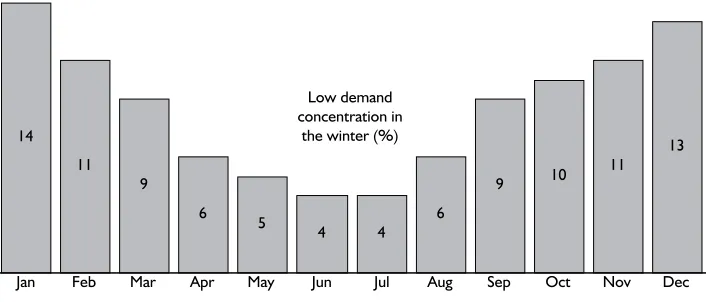
The company products are divided in three main market segments: products for immediate consume; products for consumption at home; restaurant and food service products. Its portfolio comprises almost 150 items, uniformly distributed into the three segments above. Figure 1 presents the aggregate demand profile for the current year. These data show a strong seasonal pattern on demand. The three segments present similar profiles, with slight variations.
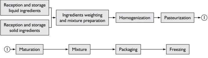
The production process can be described by some major steps showed in Figure 2. Ice cream production is a continuous process until packaging, where it is divided into several lines according to products physical characteristics.
The company operates on a “make-to-stock” strategy. Since the capacity available is insufficient to satisfy demand when it peaked, the factory built large inventories of high demand items early in the winter. The factory works 24 hours per day in three shifts. During
11 9
6 5
4 4 6
9 10 11
13
Jan Feb Mar Apr May Jun Jul Aug Sep Oct Nov Dec 14
Low demand concentration in
the winter (%)
the winter, the factory works from Mondays to Fridays, while in the summer demand peak, the factory works also on Saturdays.
Both the high capital investment and the strong seasonal demand impose some difficulties on the production planning. The large levels of inventory from both finished goods and raw materials are the ultimate motivation to this paper.
By the analysis of current production planning processes, one realizes that the main cause of the company’s high inventory levels is the disconnection between weekly production scheduling and higher-level planning processes, especially the master production planning and purchasing.
The company does not use an aggregate production planning. The current production strategy is based on operations with capacity fixed in two levels: from March to August, the factory works in 3 shifts per day, 5 days per week, from September to February, in 3 shifts per day, 6 days per week. The capacity is increased by admission of temporary employees and use of overtime. In extreme cases, production is also extended to Sunday.
In addition to the fixed capacity usage policy, the lack of detailed and accurate demand forecasts harms a proper annual Sales and Operations Planning (S&OP). In fact, the production planning uses only a Master Production Scheduling (MPS) over a 12-month horizon.
The production planning is based only on Material Requirements Planning (MRP) system (Orlicky, 1975; Baker, 1993), which determines the raw materials net demand to accomplish the MPS.
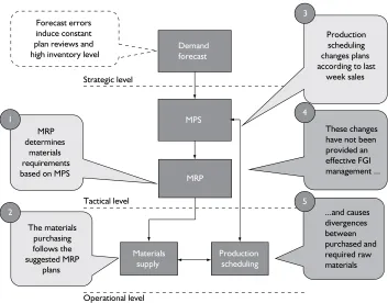
By the way, the detailed production scheduling stands on simple priority rules considering inventory levels and sales forecasts. The weekly review of sales forecast causes the divergence between the MPS and the real production schedules. Instead of promoting better service levels, it only makes worse the materials management. Figure 3 summarizes the main problems identified into the production planning process.
The objectives of this study is to provide a decision support model for aggregate production planning and to promote the planning process review in order to reduce the current inventory costs and to improve the customers service level.
1
1 Reception and storage
liquid ingredients
Ingredients weighting
and mixture preparation Homogenization
Maturation Mixture Packaging Freezing
Pasteurization Reception and storage
solid ingredients
In this paper, the issues related to forecasting and production scheduling will not be discussed. The former has been already improved by the development and implementation on spreadsheet of a forecasting model well suited to the company needs.
The production scheduling, on the other hand, imposes harder challenges, since it comprises the use of much more complex combinatorial optimization models and, by this reason, it will be postponed to a near future. A complete and useful review of the problems and models for production and scheduling in process industry is available in Kallrath (2002).
In the next section, a brief bibliographic review in aggregate production planning is presented. The formulation and details of implementation of the optimization model follow in third section. Some results from the application of the aggregate planning model and the disaggregating procedure for master production scheduling are also presented. Finally, the last section concludes this paper, presenting an analysis of main results and next steps.
Theoretical Background
The production planning process is usually divided in three levels, corresponding to the long term planning (strategic), medium term planning (tactic) and short term (operational). A classic approach to deal with this decision process in different
Production scheduling Materials
supply
Demand forecast
MPS
MRP
Tactical level
Operational level Strategic level
MRP determines
materials requirements based on MPS
1
The materials purchasing follows the suggested MRP
plans
2
Forecast errors induce constant plan reviews and high inventory level
Production scheduling changes plans according to last
week sales
These changes have not been provided an effective FGI management ...
4
...and causes divergences between purchased and required raw materials
5 3
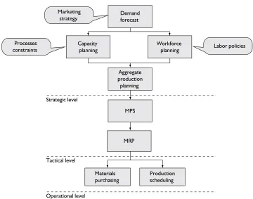
levels is the “Hierarchical Production Planning” (HPP), which was early proposed by Bitran et al. (1981). By this approach, higher level decisions constrain the lower levels, and conversely, decisions in an inferior level feedback superior process in the hierarchy. Data are aggregated due to the large number of variables, parameters and information to be considered. Besides, aggregation improves demand forecast, eases data gathering and decision analysis. Figure 4 shows a production planning hierarchy model adapted from Hopp and Spearman (2000).
Aggregate Production Planning (APP) determines the best way to meet forecast demand by adjusting the production, inventory, labor and other resources levels, over a given planning horizon typically from 6 to 18 months (Hax and Candea, 1984). This intermediate planning level is more critical when the manufacturing company produces according to a “make-to-stock” strategy, with high seasonality on demand and/or on raw material supply. Lapide (2004) discusses the S&OP from a managerial perspective and states that manufacturing companies are more aware of its importance to their business performance.
Production scheduling Materials
purchasing Demand forecast
MPS
MRP Strategic level
Tactical level
Operational level
Aggregate production planning Capacity
planning Workforce planning Processes
constraints Labor policies
Marketing strategy
There are three basic production strategies to consider, according to the demand profile and the company’s logistic costs (Chase et al., 1998):
a) Chase strategy: in this strategy, production volumes change according to demand. This requires a high flexible production system. The inventory levels tend to be lower, but with higher labor costs. In addition, the high turnover associated to chase strategy may cause negative impacts on the work force;
b) Level strategy: conversely, the level strategy seeks a smooth production capable to achieve total demand volume in planning horizon, with a constant workforce. Demand fluctuations are absorbed by finished goods inventories (FGI). As a result, the main production cost is the inventory cost. The pitfall of this strategy is the demand forecasts uncertainties and the related risk of surplus and out of stock products; and
c) Mixed strategies: the third strategy combines advantages of two previous alternatives, balancing inventory and production costs with some capacity fluctuation during the year. In this strategy, the company normally uses overtime, temporary workforce and outsourcing. Additionally, incomplete achievement of demand in peaks can be accepted.
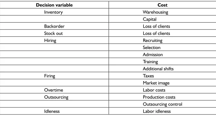
In this scenario, the mathematical programming models play an important role in balancing the trade-offs into the production planning decisions. Table 1 presents some decision variables, which must be considered in this process.
Since Holt et al. (1960) proposed its “linear decision model”, researchers in operations research community have developed a number of exact and heuristics models to solve
Table 1 - Decision variables and cost in aggregate planning.
Decision variable Cost
Inventory Warehousing
Capital
Backorder Loss of clients
Stock out Loss of clients
Hiring Recruiting
Selection Admission Training Additional shifts
Firing Taxes
Market image
Overtime Labor costs
Outsourcing Production costs
Outsourcing control
the aggregate production planning problem. These aggregate planning models can be classified as follow:
• Linear programming models: are the simplest models used in aggregate planning, which permit inclusion of several linear constraints and a large number of decision variables;
• Mixed Integer and Linear Programming (MILP): are similar to previous ones, including integer variables. The addition of integer variables further increases modeling capability, but makes the exact solution more difficult to find; and • Heuristic methods: are used when the problem cannot be solved by optimizing
algorithms efficiently. The heuristics methods are particular useful to solve the more complex MILP production planning and scheduling models.
Nam and Logendran (1992) present a comprehensive review of models and methods in aggregate planning. The basics of aggregate planning are also found in Chase et al. (1998), Nahmias (1997) and Vollmann et al. (1997) to name a few. An application of aggregate planning and scheduling in the food industry can be found in Tadei et al. (1995). Although the aggregate planning models are flexible enough to provide representative decision support to manufacturing company, they are not wide spread in real practices (Buxey, 2005).
Buxey (2003) argues that the majority of companies tend to adopt a “chase strategy”, avoiding commitment with high seasonal stocks. Piper and Vachon (2001) state that the aggregate planning literature fails to account correctly for productivity losses incurred by employee layoffs and hires. Bradley and Arntzen (1999), on the other hand, say that company should include in aggregate models some capacity decisions, since investments in inventory and equipments are equivalent in many cases.
Since the aggregate planning models demand a large amount of data, it should be integrated within the company’s information system to work properly. The operations research practitioners should be conscious of the potential and challenges trigged by the dissemination of enterprise resources planning system in the late nineties (Robinson and Dilts, 1999). In particular, one way to ease implementing operations research models is by the use of spreadsheet, the usual platform of operations managers (Grossman, 2002; Savage, 1997). Spreadsheets are clearly a solid platform for OR/ MS. Silva et al. (2006) present an interactive decision support system for production planning that uses a mixed integer linear programming model with a spreadsheet interface.
Modeling
This section describes the model developed to solve the stated aggregate production planning problem. Prior to this project, the company has already reviewed its demand forecasting process that now provides reliable aggregate monthly demand forecasts for production planning. Demand forecasts and the other input data as costs and production rates should be carefully estimated; otherwise, the results achieved by the aggregate production planning model will be useless (“garbage in, garbage out”).
Aggregate planning is the middle term production planning level. The model proposed considers a planning horizon of 12 months and solutions should be monthly reviewed (rolling-horizon) due to planning uncertainty.
The following assumptions were considered in the model development: • Safety stocks are determined outside the model (input data); • Outsourcing costs include production and material costs; • Inventory costs are evaluated at the end of each period (month);
• Normal available capacity corresponds to sum of weekdays’ three shifts production capacity, including the nighttime shift; (according to the managers, it is not economical to interrupt the production overnight and there are no relevant differences in production cost when compared with day-time shifts);
• Since the factory produces 24 hours per day during weekdays (normal shifts), extra production capacity is limited to the Saturdays’ three shifts of the month (12 or 15 shifts). Sundays and holidays are not available to production for modeling purposes; and
• Each line needs a team with a fixed number of employees. The line start up is conditioned to availability of a complete team, working a normal shift with possible overtime on Saturday.
The aggregate planning model involves all relevant decision variables to the production planning in this level of production planning hierarchy, which are listed bellow:
• Production volume (in normal shifts, overtime and outsourced) of each family in each month of planning horizon;
• Inventory volumes of each family in each month of planning horizon; • Lines which must start up in each month in normal shifts and overtime; • Number of day in normal shifts which must be used in each production line; • Number of overtime shifts which must be used in each production line; and • Workforce needed in each month to the operation of started up lines.
Index:
i Product family j Production line t Period (month)
Parameters:
ri net profit per unit of the family i dit demand of the family i during month t
ssit safety stock of family i during month t mi material cost for family i
si subcontracting cost for family i
ei cost to hold one unit of family i for one month w regular time work force cost per worker (salary) w’ cost of overtime per work-hour
h hiring cost f firing cost
pj variable costs for line j (not including work force costs)
cjt normal production capacity at line j during month t cexjt extra production capacity at line j during month t
c’it available production capacity under subcontracting during month t
aij required production time for family i at line j bj work-force needed to operate line j
Decision variables:
Sit amount sold of family i in month t
Xijt production of family i, at line j, during month t, under regular time Xit total production of family i during month t, under regular time Yijt production of family i, at line j, during month t, under extra time Yit total production of family i during month t, under extra time X’it total subcontracting production of family i during month t
Iit inventory level of family i at the end of month t Njt normal shifts of production in line j during t Ojt overtime shifts of production in line j during t Wt workforce available during month t Ht workforce hired at month t
Ft workforce fired at month t
Ajt binary variable indicating if line j is opened or close for regular time, during month t A’jt binary variable indicating if line j is opened or close for overtime, during month t
The model can be described by the following: Maximize:
r Si it m X Y s X’
t 1 T
i 1 m
i it it
t 1 T i 1 m i it t 1 T i 1 m
¤
¤
¤
¤
( )¤
¤
¤
¤
¤
¤
e Iw W (h H f F w’ b O
i it t 1 T i 1 m t t 1 T t t t 1 T j jt t 1
) TT
j 1 n
jt jt j
t 1 T
j 1 n
N O p
¤
¤
¤
¤
( )
Sitbdit
i = 1, ..., m
t = 1, ..., T (2) Xit Xijt
j 1 n
¤
i = 1, ..., mt = 1, ..., T (3)
Yit Yijt
j 1 n
¤
i = 1, ..., mt = 1, ..., T (4)
Iit Iit-1XitYitX’itSit i = 1, ..., mt = 1, ..., T (5) Iit rssit
i = 1, ..., m
t = 1, ..., T (6) Njt a Xij ijt
i 1 m
¤
j = 1, ..., nt = 1, ..., T (7)
Ojt a Yij ijt i 1
m
¤
j = 1, ..., nt = 1, ..., T (8)
Njt bc Ajt jt j = 1, ..., nt = 1, ..., T (9)
Ojt bcex A’jt jt j = 1, ..., nt = 1, ..., T (10)
X’it bc’it i = 1, ..., mt = 1, ..., T (11)
Ajt bj W
j 1 n
t
b
¤
3 i = 1, ..., mt = 1, ..., T (12)
Wt Wt-1Ht Ft t = 1, ..., T (13)
Ajt, A’jt binary j = 1, ..., n
t = 1, ..., T Wt, Ht, Ft integer non-negatives t = 1, ..., T
Sit, Xit, Xijt, Yit, Yijt, X’it, Iit, Njt, Ojt non-negatives
i = 1, ..., m j = 1, ..., n t = 1, ..., T
The objective function (Equation 1) represents the gross margin, which is the total revenue from sales subtracted by the operational costs. Theses costs are the material costs, subcontracting and inventory costs, regular and overtime workforce productions costs, hiring and firing costs and other variable costs.
Equations 2 to 13 in addition to the binary, integer and non-negatives, constitute the set of constrains of the mathematical model. The first one, Equation 2, limits the sales of each family to the respective maximum forecasted demand.
Equations 3 and 4 sum up the total month family production under, respectively, normal shifts and overtime (weekend) shifts.
The material flow balance is constrained by Equation 5. The inventory of family i at the end of month t is set equal to the respective inventory at the end of the previous month, plus the amounts produced under regular and extra time, plus the amounts produced by third parts providers, and minus the expected month sales.
Equation 6 imposes that the inventory level never remains below the safety stock level previous stated.
Equations 7 and 8 determine, respectively, the number of normal shifts (“N”) and overtime shifts (“O”) required for the production quotas, considering the available capacity of each line and the time consumption of each family.
Equations 9 and 10 restrict the maximum number of shifts (capacity) available in each line, for each month, while Equation 11 restricts the subcontracted volume to the third-part providers’ capacity.
Equation 12 imposes the requirements of workforce to operate a line. The number of employees is multiplied by three, which corresponds to the number of daily shifts if the line is opened.
Equation 13 balances the number of employees in each month, considering the hired and fired worker.
The model was implemented in MS Excel™ and solved by the optimization add-in what’s
best™. This choice was due to the user-friendly interface and the popularity of the platform
in the company. This should contribute to the project success, as argued Savage (1997).
Results
In order to validate the model, tests were conducted, considering two production lines which currently produces almost 25 items and it is quite representative of the other sectors in the factory. The products were clustered into four families of products, according to production times and demand patterns.
The tests simulated the period from January to December, and focus on: • Inventory policy and safety stocks;
• Capacity management (shifts work); • Demand priorities;
• Production strategies (Chase x Level); and • Hiring and firing decisions.
all families considered, the company should keep in inventory an amount of products equivalent to 18 days of average demand, much less than the actual level of 129 days.
Besides that, with improvements in the material management, limiting changes in master plans and detailed scheduling, the reduction should be achieved in the raw materials e packing materials inventory as well.
Lines capacity utilization
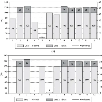
The results in Figure 5 show the use of capacity suggested by the model for the scenario considered (January to December), without considering the subcontracting alternative.
The adoption of overtime only between September and February seems inadequate to the present levels of demand. The plans provided by the model suggest using overtime in
Figure 5 - Capacity usage and workforce (no subcontract allowed). a) line 1; and b) line 2.
100 100 100 100 100 100 100
20 25 24 18 17 20 19
77
64
5
100 92
0 20 40 60 80 100 120 140
1 2 3 4 5 6 7 8 9 10 11 12 0
10 20 30 40 50 60
(%)
Line 1 - Normal Line 1 - Extra Workforce
100 100 100
4
100 100 100 100 100 100
20 25 24 18 17 20 19
0 20 40 60 80 100 120 140
1 2 3 4 5 6 7 8 9 10 11 12 0
10 20 30 40 50 60
(%)
Line 1 - Normal Line 2 - Extra Workforce 0
(a)
other months too, to avoid incurring in inventory costs, even considering not open the line (regular time) during some months. Of course, this conclusion depends on the unit inventory costs provided by the company.
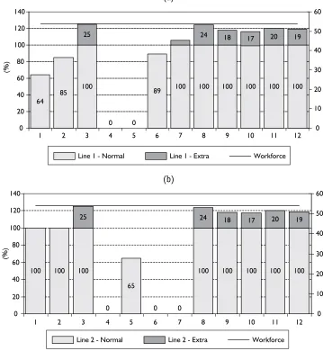
Indeed, the constant use of overtime by the company suggests the need to evaluate the opportunity of increasing the production capacity. For example, with a raise of 10% in the global demand, there is no feasible solution, i.e., the plans provided by the model cannot attend all the demand. Figure 6, on the other hand, shows the usage for a reduction of 10% in the global demand.
85 100 100 100 100 100 100
25 24 18 17 20 19
64
0 0
89 100
0 20 40 60 80 100 120 140
1 2 3 4 5 6 7 8 9 10 11 12 0
10 20 30 40 50 60
(%)
Line 1 - Normal Line 1 - Extra Workforce
100
100 100
65
0
0 0
100 100 100 100 100
25 24 18 17 20 19
0 20 40 60 80 100 120 140
1 2 3 4 5 6 7 8 9 10 11 12 0
10 20 30 40 50 60
(%)
Line 2 - Normal Line 2 - Extra Workforce
Figure 6 - Capacity usage for and workforce 90% of actual demand (no subcontract allowed). a) line 1; and b) line 2.
(a)
Due to uncertainties on demand, the production process should be reviewed each month, with the use of the aggregate planning model in a rolling horizon scheme. Some tests were done simulating this dynamic and, with minor changes in demand forecasts, the new plans can differ significantly from month to month. These kind of planed changes are expected and necessary.
Another aspect that can be evaluated with the model is the effect of forecasting accuracy in the company performance. If the company reduce the forecast error by 50%, it is expected an improvement of 10% in the gross margin. This result was achieved with the application of the aggregate planning model. The reduction in the expected error is reflected in the safety stock levels, which are inputs to the optimization model.
After the validation and implementation of the aggregate planning, the next step toward a real closed-loop planning process is the development of a disaggregating procedure that would translate the aggregate plans into a master production scheduling.
In this project, it was used a simple disaggregating procedure suggested by Hax and Candea (1984). In this basic procedure, one seeks to distribute the total family production volume by the items so that all items have equal covertures. The quantities to be produced of each family item will depend on the initial stock and its own demand forecast.
Since the aggregate planning has already considered a full year horizon, it is adopted a horizon of three months only, which is sufficient to accomplish materials and production management needs. In the literature review, it was found more sophisticated models for disaggregating plans. This will be considered in future works.
Conclusions
This paper had its focus on inventory management in a food manufacturer with a high seasonal demand. Currently, to deal with the high seasonality, the company operates with two levels of capacity, working with overtime and subcontracting during the summer. This study shows that the current strategy can be inadequate and that the company should consider a more flexible strategy in order to manage better its assets.
One problem identified was the usual practice of rescheduling production every week according to demand fluctuation. This practice causes a decoupling between materials management and production scheduling, resulting in poor inventory management as well operational inefficiency. In order to improve the company’s supply chain process, it was proposed a revision of the present sales and operations planning, emphasizing the need of working with aggregate data and linear programming model. In spite of their apparent complexity, the implementation of the models inside the revised process will contribute to reduce inventory levels in the company studied.
planning. The results achieved so far should encourage the company to extend the model and incorporate them into its production planning process.
References
Baker, K. R. (1993), Requirements Planning. In: Graves, S. C. et al. (Eds.) Handbooks in Operations Research and Management Science, Vol. 4, North-Holland, Amsterdam. pp. 571-627.
Bitran, G. R.; Haas, E. A.; Hax, A. C. (1981), Hierarchical Production Planning: a single stage system. Operations Research, Vol. 29, No. 4, pp. 717-743.
Bradley, J. R.; Arntzen, B. C. (1999), The simultaneous planning of production, capacity, and inventory. Operations Research, Vol. 47, No. 6, pp. 795-806.
Buxey, G. (2003), Strategy not tactics drives aggregate planning. International Journal of Production Economics, Vol. 85, No. 3, pp. 331-346.
Buxey, G. (2005), Aggregate Planning for seasonal demand: reconciling theory with practice. International Journal of Operations and Production Management. Vol. 25, No. 11, pp. 1083-1100.
Chase, R. B.; Aquilano, N. J.; Jacobs, F. R. (1998), Production and Operations Management: manufacturing and services (8th edition). Irwin/McGraw-Hill, New York. 889 p. Clark, A. R.; Clark, S. J. (2000), Rolling-horizon lot-sizing when set-up times are
sequence-dependent. International Journal of Production Research, Vol. 38, No. 10, pp. 2287-2307.
Grossman, T. A. (2002), Spreadsheet add-in for OR/MS. ORMS Today, Vol. 29, No.4. Hax, A. C.; Candea, D. (1984), Production and Inventory Management. Prentice-Hall,
Englewood Cliffs, New Jersey. 513 p.
Holt, C. C.; Modigliani, F.; Muth, J. F.; Simon, H. A. (1960). Planning Production, Inventory and Work Force. Prentice Hall, Englewood Cliffs, New Jersey. 433 p.
Hoop, W. J.; Spearman, M. L. (2000) Factory Physics: foundations of manufacturing management (2nd ed.). Irwin/McGraw-Hill, New York. 698 p.
Kallrath (2002), Planning and scheduling in the process industry. OR Spectrum, Vol. 24, No. 3, pp. 219-250.
Lapide, L. (2004), Sales and Operations Planning: the process. The Journal of Business Forecasting, Vol. 23, No. 3, pp. 17-19.
Nahmias, S. (1997), Production and Operations Analysis (3rd ed.). Irwin, Chicago. 858 p.
Nam, S.; Logendran, R. (1992), Aggregate production planning: a survey of models and methodologies. European Journal of Operational Research, Vol. 61, No. 3, pp. 255-272. Orlicky, J. A. (1975), Material Requirements Planning: the new way of life in production
and inventory management. McGraw-Hill, Nova York. 292 p.
Robinson, A. G.; Dilts, D. M. (1999), OR & ERP: a match for the new millennium? ORMS Today, Vol. 26, No. 3.
Savage, S. (1997), Weighing the Pros and Cons of decision technology in spreadsheets. ORMS Today, Vol. 24, No. 1.
Silva, C. G.; Figueira, J.; Lisboa, J.; Barman, S. (2006), An interactive decision support system for an aggregate production planning based on multiple criteria mixed integer linear programming. Omega, Vol. 34, No. 2, pp. 167-177.
Tadei, R.; Trubian, M.; Avendaño, J. L.; Della Groce, F.; Menga, G. (1995), Aggregate planning and scheduling in the food industry. European Journal of Operational Research, Vol. 87, No. 3, pp. 564-573.
Vollmann, T. E.; Berry, W. L.; Whybark, D. C. (1997), Manufacturing Planning and Control System (4th ed.). McGraw-Hill, New York. 896 p.
Biography
Flávia Midori Takey has recently completed her Bachelor’s degree in production engineering from the Polytechnic School of the University of São Paulo (USP). Her professional interest focuses on logistics and production management.
Marco Aurélio de Mesquita is assistant professor of logistics and operations management at the Polytechnic School of the University of São Paulo (USP), in Brazil. He holds a BS and MS degree in naval engineering and a PhD degree in production engineering from the Polytechnic School (USP). His research interests include modeling and simulation of production systems, inventory management and production scheduling. He is a member of the ABEPRO (The Brazilian Association for Production Engineering) and of the INFORMS.
Submitted: 6th February, 2006.