Comparison of Different Configurations of Ranney Wells Using Finite
Element Modeling
M. Dimkić1, M. Krstić1,2, N. Filipović2, B. Stojanović2, V. Ranković2, L. Otašević2, M.
Ivanović2, M. Nedeljković2, M. Tričković1, M. Pušić1, Đ. Boreli-Zdravković1, D. Đurić1,
M. Kojić2
1Institute for Development of Water Resources “Jaroslav Černi”,
Jaroslava Černog 80, 11226 Belgrade, Serbia e-mail: [email protected]
2Center for Scientific Research of Serbian Academy of Science and Arts and University of
Kragujevac,
University of Kragujevac, Jovana Cvijića bb, 34000 Kragujevac, Serbia and Montenegro e-mail: [email protected]
Abstract
The objectives of this study are to define the regional and local groundwater flow, and to give quantitative estimates of different dynamic parameters for Ranney wells in Belgrade Water Supply Center. To solve these tasks used the numerical tools to quantitatively model flow through porous saturated and unsaturated media. We used finite element (FE) modeling of underground water flow and developed specific algorithms for the Ranney wells representation. The unsaturated soil hydraulic properties are described for each finite element by applying our 3D interpolation algorithm. Our software for pre- and post-processing Lizza is used, developed for easy modeling of complex engineering underground water flow problems with Ranney wells. The software FE package PAK-P is employed as the solver. This software can handle flow regions delineated by irregular boundaries. The flow region may be composed of nonuniform soils having an arbitrary degree of local anisotropy. Flow can occur in the vertical plane, the horizontal plane, or in a three dimensional region exhibiting radial symmetry about the vertical axis. Constant or time-varying prescribed head and flux boundaries can be handled, as well as boundaries controlled by atmospheric conditions. Soil surface boundary conditions may change during the simulation from prescribed flux to prescribed head type conditions (and vice versa). A seepage face boundary through which water leaves the saturated part of the flow domain can be modeled, and also free drainage boundary conditions. The results of simulation for some real engineering problems (Ranney well RB-8 in Belgrade Water Supply Center) are presented.
1. Introduction
The goal of underground water flow analysis is determination of the field of flow potential (pressure) and the field of fluid velocity for given boundary conditions. In general, these physical fields are functions of time. For a fluid through porous medium in the domain of small velocities, Darcy’s law is considered fundamental. On the basis of this law and continuity equation for fluid, the basic differential equation for stationary and non-stationary problems can be derived. Before computers, this differential equation was solved in analytical form for certain simple boundary conditions.
Numerical solutions of fluid flow through porous media were firs based on the finite difference method. This method is not practical for complex boundary conditions and especially for 3D problems. However, with development of the finite element method (FEM), first in solid mechanics (structures), and with generalizations to general field problems, a large number of complex theoretical and practical problems were solved. Problems of fluid flow through porous media were among these field problems. Special procedures were developed for solving specific tasks related to underground water flow.
In this paper, we focus on modeling Ranney wells using the finite element method. We present a number of specific procedures in modeling 3D problems with general boundary conditions, including variable material characteristics of porous media.
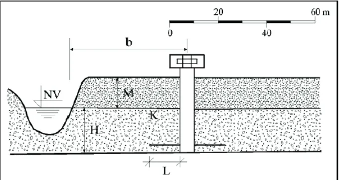
1.1 Ranney wells.
The Ranney wells consist, in general, of vertical concrete caisson, with depth between 20 and 25 meters, and radius between 4 and 5 meters (Fig.1). In the lower part of caisson holes are drilled, usually eight, through which horizontal well screens are inserted into the aquifer. Well screens are perforated pipes, through which underground water enters the well. Length of well screens is usually 40 to 50 meters, and the radius is 0.2 m.
2. Theoretical background
The basic quantity from which we start in fluid flow through porous medium is potential φ defined as [1]
p h
φ γ
= + (1)
where p is fluid pressure, γ – specific weight, and h is height in vertical direction measured with respect to a adopted reference plane. Fluid velocity q, also known as Darcy’s velocity, represents the fluid volume which passes in unit time through a unit area of porous medium. This velocity is related to the potential as
φ = − ∇
q K (2)
where K is the diagonal permeability matrix. Then, the continuity equation for non-stationary conditions can be written as
2 2 2
2 2 2
x y z
k k k Q S
t
x y z
φ φ φ φ
∂ + ∂ + ∂ + = ∂
∂
∂ ∂ ∂ (3)
where kx, ky, kz are coefficients of the matrix K, Q is the volumetric flux, and S is the
storage.
In the case of the existence of free surface, we have that the points for which the condition
h
φ ≤ (4)
is satisfied, the points are below or on the free surface. For points above the free surface we correct the permeability matrix, as
0
us
= −
K K K (5)
where the matrix K0 is the matrix for points below the free surface, and 0
us=α
K K , with the coefficient α<1 ( we use α=0.999).
The balance equation for a (3D) finite element in case of incremental-iterative scheme (for non-stationary conditions with free surface) can be written as [2]
( 1)
( ) ( 1)
1 i e i
t t e t t e t t e i
t φφ φ φ − +Δ +Δ +Δ − ⎛ + ⎞ Δ = ⎜ Δ ⎟
⎝ K S ⎠ f (6)
where
T T T
e
x y z
V
k k k dV
x x y y z z
φ φ φ φφ φ φ φ ⎡ ∂ ∂ ∂ ∂ ∂ ∂ ⎤ = ⎢ + + ⎥ ∂ ∂ ∂ ∂ ∂ ∂ ⎢ ⎥ ⎣ ⎦
∫
H H HK (7)
e T
A
S φ φdV = −
∫
S H H (8)
Here Hφ isthe interpolation matrix, Δt is time step, Δφe i( )is the vector of increments of nodal potentials. The vector t t e i( 1)
φ
+Δf − depends on the solution from the previous iteration and
counter within time step, respectively. For specific application in modeling of Ranney wells, 1D element has been developed, with the element matrix
T e
x L
k dL
x x
φ φφ
φ ∂ ∂ =
∂ ∂
∫
HK (9)
2.1 Modeling well screens using 1D elements
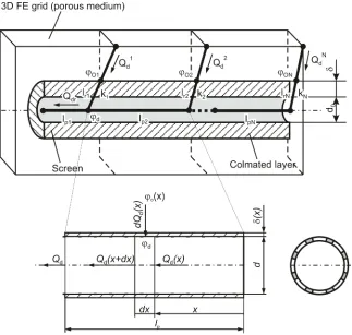
We use 1D elements to represent the screens. The screen is divided into screen segments where each segment is modeled by an axial 1D element. In order to perform this approximation without deviation from the continuity condition, we introduced radial 1D elements which represent connection between screen and porous medium modeled by 3D elements (Fig. 2).
Fig. 2. A schematic representation of a well screen with axial and radial finite elements.
The main task was to determine permeability of the radial 1D elements which take into account permeability of colmated layer, length of the axial 1D element and diameter of the screen. In order to achieve this, consider a well screen segment with the length lp (Fig. 2). The relations between volumetric fluxes j
( )
d
Q x and j
(
)
dQ x dx+ at a positions x and x+dx of the screen segment “j” can be related as
(
)
( )
( )
j j j
d d d
The flux increment j
( )
ddQ x can further be expressed in the form
( )
( )
j j j
d p
dQ x =v x dP (11)
where j p
dP is the elementary surface of the screen through which water is entering the screen, and v xj
( )
is the entering radial velocity. Next, we express the surface jp
dP using the surface ratio j
p
r (area of holes divided by the total area of the screen segment surface), as
j j
p p
dP =d r dxπ (12)
where d is the screen diameter. Further, we have the relation
( )
( )
j j j
d p
dQ x =d r v x dxπ (13)
The following relationship follows from Darcy's law
( )
( ) ( )( )
oj dj j
j x v x k x
x
ϕ ϕ
δ −
= (14)
where k xj
( )
is the permeability of the surrounding filtration layer, which takes into accountthe conditions at the screen holes; δj
( )
x is the thickness of the surrounding filtration layeraffecting the flow within the screen segment; ϕoj
( )
x and ϕd are potentials in the surroundinglayer and inside the screen segment at the coordinate x. Then, from the above equations we obtain the flux through the screen segment as
( )
( )
(
( )
)
0 j p l j j jd p j oj d
k x
Q d r x dx
x
π ϕ ϕ
δ
=
∫
− (15)where j p
l represents length of screen segment.
Since the dimensions of the screen segment is small with respect to the whole flow region, we neglect change of ϕoj with respect to the axial coordinate x and take
( )
.oj x oj const
ϕ =ϕ = (16)
where ϕoj is the potential in the screen segment surrounding. Therefore, for a screen “j” we can write the relation
(
)
( )
( )
0 j p l j j jd p oj d j
k x
Q d r dx
x
π ϕ ϕ
δ
= −
∫
(17)Finally, we express the screen segment hidraulic resistance j d
R using the relation
(
)
/j j
d oj d d
Q = ϕ −ϕ R (18)
( )
( )
0
1/
j p
l j
j j
d p j
k x
R d r dx
x π
δ
=
∫
(19)The line integral of the ratio k xj
( )
/δj( )
x can be obtained as a sum of the integrals withpartially constant ratios along the screen segment length. If this ratio is constant along the screen segment length, then the screen segment permeability can be obtained in a simple form
1/ j j j j j
d p p j
k R d πr l
δ
= (20)
2.2 Well model
We model each screen by a number of line elements along the length and connect each of these screen nodes to the closest 3D mesh node using two radial 1D elements. First of them represents the surrounding filtration layer, and the second connects the first 1D element with the 3D mesh. The axial 1D elements have a selected (high) permeabilities. Using Eq. (20) we obtain permeability of the radial element of the screen segment ’j’ as
j
j j j
ss p p j
k
k d r lπ
δ
= (21)
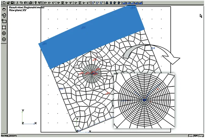
We use a non-structured mesh, and represent the well screens by 1D elements, which are inserted in the 3D mesh (Fig. 3). The non-structured mesh is obtained by Delauney triangulation, and further conversion of triangles to quads using Q-Morph algorithm. The quadrilateral mesh is refined in order to improve element quality and to avoid element degeneration.
3. Results
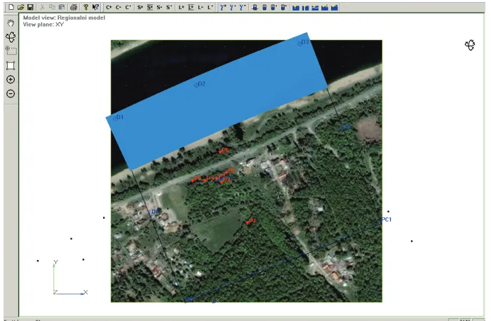
We modeled the well RB-8 near Sava lake (Belgrade Water Supply Center) assuming two configurations. First, with 3 screens (actual configuration), and the second - with 6 screens (possible configuration). Our global model includes porous medium on one side of Sava lake, with dimensions approximately 500 x 500 [m] in horizontal plane and with depth of 40 [m]. We considered steady flow conditions. The 3D FE model is generated by the preprocessor Lizza [3], based on the geological data.
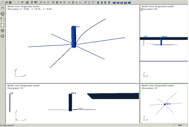
Boundary conditions consist of: impermeable bottom plane and impermeable vertical surface bounding the model; the top surface of the model is the free surface. Also, we model river by a prescribed potential at the river-soil boundary, and also we prescribe the potential at the Belgrade boundary. There are 5 additional wells (D1-D5) which simulate the global flow conditions (Fig. 4).
Fig. 4. Model of RB-8 Ranney well.
Fig. 5. Well RB-8 with 3 screens (actual configuration).
RB-8
0 10 20 30 40 50 60 70
Q well Screen 1
Screen 2
Screen 3
Screen 4
Screen 5
Screen 6
Q
[
l/s
]
3 screens 6 screens
Fig. 7. Comparison of flow through well and well screens in two different configurations.
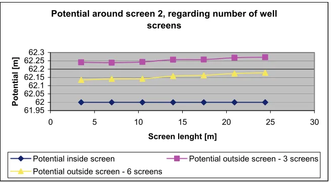
It can be noted from Fig. 7 that introducing (injecting) of three new well screens into existing Ranney well increases the total water flow through the well. However, this increase is not equal to the total flow rate of the three well screens in the actual configuration. This result can be explained by the fact that injection of new screens decreases flow rate in the existing screens. Decrease of flow rate in the existing screens is the consequence of a potential decrease in the well surrounding.
Potential around screen 2, regarding number of well screens
61.9562 62.0562.1 62.1562.2 62.2562.3
0 5 10 15 20 25 30
Screen lenght [m]
Pot
ent
ia
l [
m
]
Potential inside screen Potential outside screen - 3 screens Potential outside screen - 6 screens
Fig. 8. Comparison of potentials along screen 2 obtained for two different well configurations (3 and 6 screens).
4. Conclusion
Increase of flow rate capacity of Ranney well by injecting new screens is the basic parameter in making decision about the optimal number of screens to be used. In this paper we have shown that our software (Lizza and PAK-P [3], [4]) can be useful in solving real engineering problems of underground water flow and in managing the water resources with Ranney wells.
References
[1] Kojić M., N. Filipović, N. Zdravković, Đ. Boreli-Zdravković, D. Divac, Modeliranje filtracije podzemnih voda metodom konačnih elemenata, Upravljanje vodnim resursima Srbije ’97 189-207, 1997.
[2] Kojić M., R. Slavković, M. Živković, N. Grujović, Finite Element Method - I Linear Analysis, Faculty of Mech. Eng. Univ. Kragujevac, Kragujevac, 1998.
[3] Lizza, pre- and post-processor for modeling of underground water flow with Ranney wells, Center for Scientific Research of Serbian Academy of Science and Arts and University of Kragujevac, Institute for Development of Water Resources “Jaroslav Černi” .