Adaptive Thresholding Based On Co-Occurrence
Matrix Edge Information
M. M. Mokji
Faculty of Electrical Engineering University of Technology Malaysia, Malaysia
email: [email protected]
S.A.R. Abu Bakar Faculty of Electrical Engineering University of Technology Malaysia, Malaysia
email: [email protected]
Abstract—In this paper, an adaptive thresholding technique based on gray level co-occurrence matrix (GLCM) is presented to handle images with fuzzy boundaries. As GLCM contains information on the distribution of gray level transition frequency and edge information, it is very useful for the computation of threshold value. Here the algorithm is designed to have flexibility on the edge definition so that it can handle the object’s fuzzy boundaries. By manipulating information in the GLCM, a statistical feature is derived to act as the threshold value for the image segmentation process. The proposed method is tested with the starfruit defect images. To demonstrate the ability of the proposed method, experimental results are compared with three other thresholding techniques.
Index Terms—Co-occurrence matrix, entropy, thresholding,
edge magnitude
I. INTRODUCTION
Thresholding techniques are often used to segment images consisting of dark objects against bright backgrounds, or vice versa. It also offers data compression and fast data processing [1]. The simplest way is through a technique called global thresholding, where one threshold value is selected for the entire image, which is obtained from the global information. However, when the background has non-uniform illumination, a fixed (or global) threshold value will poorly segment the image. Thus, a local threshold value that changes dynamically over the image is needed. This technique is called adaptive thresholding.
Many works have been done to formulate the best technique for the adaptive thresholding to accommodate image conditions such as non-uniform illumination, noisy image and complex background [1-15]. Basically these techniques can be divided into region-based and edge-based thresholding. Region-edge-based technique uses the whole image to extract the information for the threshold value computation, while edge-based technique is based on the attributes along the contour between the object and the background.
For region-based technique, most of the early introduced techniques are based on the image histogram. In 1979, Otsu [2] presented a technique that considered the image histogram as having a two gaussian distribution representing the object and the background. A threshold is selected to maximize the inter-class separation on the basis of the class variances. Using the same two gaussian classes assumption, Kittler and Illingworth [3] selected a threshold value that minimized error in the Bayes sense. However, the shape of the image histogram is usually multi-modal instead of bimodal. One solution for this problem is by considering the local statistic measure of the input image [4]. These statistics include the mean value of the gray level and function obtained from the minimum and maximum values of the gray level. Apart from that, a thresholding technique, which is based on illumination-independent contrast measure, is introduced to segment outdoor scene images [1]. The primary idea of this method is to employ only the contrast measure and its threshold in a region-wise interpolation of the threshold for the adjacent regions.
thresholding is based on the co-occurrence matrix where distribution of grayscale transitions together with the edge information is embedded in the matrix [10]. From the co-occurrence matrix, several types of entropies such as global, local, joint and relative entropy are computed to determine the threshold value [10-15]. This technique is simple and easy to use because the co-occurrence matrix itself already contains most information needed for threshold value computation. However, most of the techniques do not use the edge information in the co-occurrence matrix effectively and produce poor result when dealing with noisy, complex background and fuzzy boundary images. Thus, this paper is proposing a new technique based on the co-occurrence matrix where statistical features will be defined from the edge information to handle images that have fuzzy boundaries between the object and the background of the image.
II. GRAY LEVEL CO-OCCURRENCE MATRIX
Gray level co-occurrence matrix (GLCM) has been proven to be a very powerful tool for texture image segmentation [16, 17]. GLCM describe the frequency of one gray tone appearing in a specified spatial linear relationship with another gray tone within the area of investigation [18]. Here, the co-occurrence matrix is computed based on two parameters, which are the relative distance between the pixel pair
d
measured in pixel number and their relative orientationφ
. Normally,φ
is quantized in four directions (horizontal: 00, diagonal: 450, vertical: 900 and anti-diagonal: 1350) [18]. These orientations are referred to the 4-adjacency pixels at)
,
(
x
+
d
y
,(
x
,
y
−
1
)
,(
x
−
1
,
y
)
and(
x
,
y
+
1
)
. In practice, for eachd
, the resulting values for the four directions are averaged out. To show how the computation is done, for imageI
, letm
represent the gray level of pixels(
x
,
y
)
andn
represent the gray level of pixels(
x
±
d
φ
1,
y
±
d
φ
2)
withL
level of gray tones where0
≤
x
≤
M
−
1
,0
≤
y
≤
N
−
1
and1
,
0
≤
m
n
≤
L
−
.(
φ
1,
φ
2)
is set to(
1
,
0
)
forhorizontal direction,
(
1
,
−
1
)
for diagonal direction,)
1
,
0
(
for vertical direction and(
1
,
1
)
for anti-diagonal direction. From these representations, the gray level co-occurrence matrixC
m,n for distanced
and directionφ
can be defined as
∑∑
−= −
= ⎟⎟⎠
⎞ ⎜⎜
⎝ ⎛
= ± ±
=
= 1
0 1
0 1 2
,
} ) ,
(
& ) , ( { 1 M
x N
y n
m
n d y d x I
m y x I P
R C
φ
φ
(1)where
P
{.}
=
1
if the argument is true and otherwise,0
{.}
=
P
. In words, for each of the intensity pair)
,
(
m
n
, Equation 1 counts the number of the pixel pair that occurred in the whole imageI
at relative distanced
and directionφ
. Variable R in Equation 1 normalizedthe computation. Thus, GLCM is actually represents the probability of the pixel pairs. As an example, Figure 1
shows the GLCM for
d
=
1
,φ
=
0
0 and4
=
=
=
N
L
M
where the resulting GLCM isanti-diagonally symmetry.
Figure 1. GLCM
In the classical paper [19], Haralick et. al have introduced fourteen textural features from the GLCM and then in Reference [2] stated that only six of the textural features are considered to be the most relevant. Those textural features are Energy, Entropy, Contrast, Variance, Correlation and Inverse Difference Moment. All these textural features are computed based on the frequency or repetition of the pixel pair, as it is the apparent information contains in the GLCM. However, there is another information, which is applied for the computation of a few of the textural features. It can be best described as an edge magnitude
p
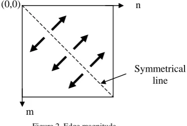
defined as gray value difference of the pixel pair. Inside the GLCM, the edge magnitude is not shown by the value of the matrix but the value of the edge magnitude is determined by the position of the pixel pair inside the GLCM. Visually, the edge magnitude increases diagonally in the GLCM as shown by the bold arrows in Figure 2
Figure 2. Edge magnitude
From Figure 2, the edge magnitude is equal to zero along the symmetrical line where
m
=
n
while the maximum value of the edge magnitude are located at)
0
,
(
l
C
andC
(
0
,
l
)
wherel
=
L
−
1
is the maximum value of the gray tone of the image. Among the six textural values defined from the GLCM, only the contrast computation includes the edge magnitude information as shown in Equation 2. This is why contrast has the ability to measure coarseness of an image. For variance and correlation, almost similar information is included. However, the edge information is computed based on the0 0
0 0
1 1
2 2
2 2 2
2 3
3
3 3
I =
4 1
0 0
1 2
1 0
0 3 2
0 1
0
6 3
Cm,n =
24
1
Symmetrical line n
current pixel pair and the mean pixel value of the image rather than based on the pixel pair alone.
∑ ∑∑
− = = − − = − =⎪⎭
⎪
⎬
⎫
⎪⎩
⎪
⎨
⎧
=
1 0 | | 1 0 1 0 2)
,
(
L p p n m L m L nn
m
C
p
CON
(2)Object in an image is visible if the boundary of the object is visible. One way of quantifying the visibility of the object’s boundary can be done by applying the edge magnitude computation. Normally, the object’s boundary will have higher edge magnitude value compare to the object region itself and the background region of the image. In GLCM, instead of the ability of representing the edge magnitude, the matrix can be partitioned into sub-regions where object, background and boundary of the object are placed in different region. These regions are called GLCM quadrants [22].
III. GLCM QUADRANTS
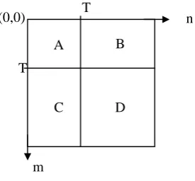
When a threshold value T is chose and mapped on the GLCM, the threshold value partitions the GLCM into four quadrants as shown in Figure 3. Quadrant A represents gray level transition within the object (dark area) while quadrant D represents gray level transition within the background (bright area). The gray level transition between the object and the background or across the object’s boundary is placed in quadrant B and quadrant C. These four regions can be further grouped into two classes, referred to as local quadrant and joint quadrant. Local quadrant is referred to quadrant A and D and it is called local quadrant because the gray level transition arises within the object or the background of the image. Then quadrant B and C is referred as joint quadrant because the gray level transition occurs between the object and the background of the image.
Figure 3. GLCM quadrants
As mentioned in the Introduction section, entropy as one of the GLCM feature is the only feature applied to determine the threshold value [10-15]. Before entropy is quantified based on GLCM, it is quantified based on gray level image histogram [23]. The drawback of this technique is lack of gray level correlation information. As
a result, two different images with identical image histogram will results similar threshold value [22]. The problem is solved when Pal and Pal introduced entropy based thresholding based on GLCM where correlation of the pixel pair is considered [13]. In their method, local entropy (
H
LE) is computed within the local quadrants.As there are two local quadrants in GLCM (quadrant A and D), two entropy values are computed for each of the local quadrant as in Equation 3 and 4.
∑∑
= =−
=
T m T nA
T
C
m
n
C
m
n
H
0 0)
,
(
log
)
,
(
)
(
(3)∑ ∑
− + = − + =−
=
1 1 1 1)
,
(
log
)
,
(
)
(
L T m L T nD
T
C
m
n
C
m
n
H
(4)The
H
LE is then derived by summing up the)
(
T
H
A andH
D(
T
)
. Based on theH
LE, Pal and Palchose the threshold value as
T
LE values specified byEquation 6, which maximize the
H
LE defined byEquation 5.
)
(
)
(
)
(
T
H
T
H
T
H
LE=
A+
D (5)⎥⎦
⎤
⎢⎣
⎡
=
−=
max
(
)
arg
) 1 ,..., 1 , 0(
H
T
T
LEL T
LE (6)
Alternatively, Pal and Pal also derived entropy called joint entropy,
H
JE (Equation 9) where it is a summation of entropy in quadrant B (Equation 7) and entropy in quadrant C (Equation 8).∑ ∑
= − + =−
=
T m L T nB
T
C
m
n
C
m
n
H
0 1 1)
,
(
log
)
,
(
)
(
(7)∑ ∑
− + = =−
=
1 1 0)
,
(
log
)
,
(
)
(
L T m T nC
T
C
m
n
C
m
n
H
(8))
(
)
(
)
(
T
H
T
H
T
H
JE=
B+
C (9)Similar to local entropy, threshold value based on the
joint entropy is selected when maximum
H
JE isachieved. This is shown in Equation 10 where
T
JE is theresulting threshold value.
⎥⎦
⎤
⎢⎣
⎡
=
−=
max
(
)
arg
) 1 ,..., 1 , 0(
H
T
T
JEL T
JE (10)
Another entropy that can be derived from the GLCM quadrants is global entropy (
H
GE), which is simply defined as the sum of the local entropy and the joint nm (0,0)
A B
C D T
entropy. The threshold value is then selected based on Equation 11.
⎥⎦
⎤
⎢⎣
⎡
=
−=
max
(
)
arg
) 1 ,..., 1 , 0(
H
T
T
GEL T
GE (11)
An extended formulation of the entropy, which is called relative entropy was also introduced [22]. It is defined by Equation 12 where
C
m,n is GLCM generatedfrom the original input image and
h
Tm,n is GLCMgenerated from the thresholded image.
∑∑
− = − ==
1 0 1 0 , , , ,,
};
{
}]
log
[{
L
m L
n Tmn
n m n m n m T n m
h
C
C
h
C
J
(12)Relative entropy in Equation 12 is actually a function that measures the distance between the input image and the result image (thresholded image). Here, good thresholded image is the one that tries to match the input image. Thus, the selected threshold value T should be the gray value that minimizes the relative entropy as described in Equation 13.
⎥⎦
⎤
⎢⎣
⎡
=
−=
max
[{
};
{
}]
arg
, ,) 1 ..., 1 , 0 ( n m T n m L T
RE
J
C
h
T
(13)IV. PROPOSED THRESHOLDING TECHNIQUE
In the previous section, it was shown how entropy in GLCM is used for thresholding. In this work, instead of entropy, information based on edge magnitude, which is found in GLCM contrast quantification will be applied for the thresholding process. Based on the edge magnitude, a new statistical feature representing the threshold value
T
is computed according to Equation 14 as follow∑ ∑
− = = +′
⋅
+
=
pm n m p
n
m
C
n
m
T
l l 0)
,
(
2
1
η
(14)where
∑ ∑
−= = +
′
=
pm n m p
n
m
C
l l 0)
,
(
η
(15))
,
(
m
n
C
′
in Equation 14 gives information on thefrequency of the pixel pair and on the other hand, the edge component is represented by the range of the two level summation operations. This summation range forces the equation to compute the threshold value within a specific area in the GLCM, which is an area restricted by
p
m
n
−
≥
. This means that the computation onlyinvolves pixel pair with the edge magnitude greater than
or equals to
p
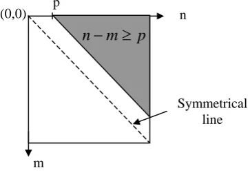
. Figure 4 illustrates the computation area (shaded area) within the GLCM. By choosing a rightp
value, the computation area will be on the object’s boundary area. This area is differs from the GLCM quadrants where the object’s boundary area is placed in quadrant B and C. As the proposed technique compute the threshold value based on edge magnitude, regions in the GLCM are separated diagonally rather than separating it into four different rectangular as in the GLCM quadrants.
From Figure 4, It can also be seen that the computation area is only assigned to the upper triangle of the GLCM although area with edge magnitude greater than or equal to
p
also exist at the lower triangle. The reason is to reduce the computation burden as both areas at the upper and lower triangles have similar values due to the symmetrical feature of the GLCM.Figure 4. Threshold computation area
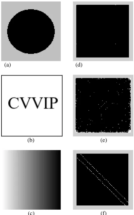
To illustrate the difference between the entropy based method and the proposed method, Figure 5 shows three basic images and its GLCM mapping. Brighter points in the GLCM represent higher value of the GLCM components or higher repetition of the pixel pair occurrence. Figure 5(a) is a two color image, Figure 5(b) shows an image with low blurred effect and Figure 5(c) is a horizontal gradient effect image where the image pixel value changes uniformly in the horizontal direction.
In the entropy based method, the T value is chosen based on the most uniform or lowest randomness texture of the input image in the joint quadrants [13]. Higher value of entropy contributes to more uniform texture. Thus, the resulting T value for image in Figure 5(a) is equal to 0 where white points at the upper left, upper right and lower left of its GLCM mapping were included in the computation. The thresholding result is perfect where pixel value less than or equals to zero becomes 0 and the rest becomes one. For image in Figure 5(b), entropy based thresholding results a threshold value equals to 0.92. Its thresholding in Figure 6(b) shows a poor thresholding. This is because the most uniform texture for the joint quadrants in the GLCM is near to the right and bottom limit of the GLCM. However, pixels value bounded by the joint quadrants have most values from 0 to 1. Thus, the resulting threshold value does not precisely represent the boundary’s pixel values. Problem Symmetrical line n m (0,0)
p
m
n
−
≥
also occurred if the entropy based thresholding is applied to the image in Figure 5(c) because the obtained GLCM contained only nonzero values mapped diagonally on it. With this pattern of GLCM mapping, for most gray values, entropy value computed in the joint quadrants will be similar. Thus the threshold value will be too low if the first maximum entropy is considered or the threshold value will be too high if the last maximum entropy is considered. Figure 6(c) shows the thresholding results when the first maximum entropy is considered. This is a poor thresholding since only a small part of the image becomes dark.
(a) (d)
(b) (e)
(c) (f)
Figure 5: Basic shapes and their GLCM mapping. (a) Two color image, (b) Blurred image, (c) Gradient image, (d)-(f) respective GLCM
mapping for image (a)-(c)
As for the proposed technique, the computation area is depends on the edge magnitude rather than the GLCM quadrants. In the proposed technique, only the computation area is referred to the GLCM while the threshold value computation is totally based on the gray values of the input image (first order statistic feature). This is varying with the entropy based technique where both the computation area and the threshold value computation are based on the GLCM pixel pair repetition (second order statistic feature). Thus a more precise representation of the pixel values on the boundary of the
(a) (d)
(b) (e)
(c) (f)
Figure 6: Thresholding results for image In Figure 5(a) to 5(c). (a)-(c) Results based on entropy method respectively, (d)-(f) Results based
on the proposed technique.
quadrants for any gray levels value, the proposed technique includes the entire GLCM elements in its computation area. Thus, average value of the gray values gives a good threshold value where the input image is segmented evenly with bright and dark pixel as shown in Figure 6(f).
Another parameter included in the threshold value
T
formulation isη
, defined as the total number of pixel pairs within the GLCM with the edge magnitude higher than or equal top
. Dividing the formulation withη
translates theT
value to have a similar function with the image gray value. This process is also called normalization where theT
value is placed within0
to1
−
L
. Back to Equation 1, normalization is also applied in the GLCM computation by dividing the formulationwith
R
. In the proposed technique, the GLCMnormalization with
R
is ignored and replaced with the normalization based onη
in Equation 14. Thus, GLCM used in Equation 14(
C
′
(
m
,
n
))
is not normalized. Replacing the normalization function is done because the summation range in Equation 14 has been altered based on the shaded region in Figure 4 while the summation range for GLCM in Equation 1 is the whole GLCM. By adopting the normalization in the Equation 14, the thresholding process can be applied straight from theT
value. This circumstance gives an advantage to the proposed technique compared to the other co-occurrence matrix based thresholding techniques [10-12] where a nonlinear transformation from the computed parameter from the GLCM is required prior to the thresholding process. The nonlinear transformation is done by selecting a gray value as a threshold value that maximizes or minimizes the parameter (Equation 6, 10, 11, 13).
The most significant feature in the proposed technique is its flexibility, which is denoted by variables
d
andp
. This flexibility gives the ability to handle either solid or fuzzy edges where wider pixel distance is occupied by the edges. Here, by changing the value ofd
(relative distance between the pixel pair) and
p
(edge magnitude) will change the sensitivity of the edge definition in the thresholding process. The greater the fuzziness of the edges need higherd
andp
. In previous work, such flexibility is also described in Reference [15]. However, the edge detection process and selection of the suitable threshold value is done separately while in this work, both processes are combined in one equation. In Reference [15], flexibility in its edge detection process is possible as it uses the Laplacian operator where the output depends on the selected standard deviation (σ
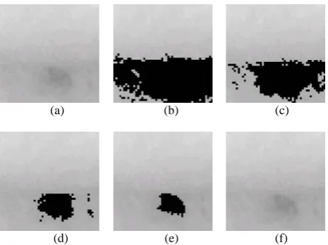
). Figure 7 illustrates the results of the thresholding process on starfruit skin with various values ofd
andp
.The purpose of the thresholding process in this work is to segment the defect area on the starfruit skin. The starfruit skin image is chosen because defects on its surface have fuzzy edges as in Figure 7. The defect in the
image is not properly segmented when the distance between the pixel pair and the edge magnitude is too small (Figure 7(b) & 7(c)). The best segmentation result
is achieved when
d
andp
are set to 3 and 5respectively (Figure 7(e)) where edge is defined with wider pixel and higher edge magnitude. However, when
p
is set at a very high value (Figure 7(f)), no defect issegmented. This is because in this case,
C
(
m
,
n
)
usually has a zero value and causes the threshold valueT
to become infinity.
(a) (b) (c)
(d) (e) (f)
Figure 7. Segmentation, (a) original image, (b) d=1 p=1, (c) d=2 p=2, (d) d=2 p=3, (e) d=3 p=5, (f) d=3 p=12.
V. EXPERIMENTAL RESULTS
computation to select the threshold value. As for our method, we set
d
= 3 andp
= 5.) , ( 4 ) 1 , (
) 1 , ( ) , 1 ( ) , 1 ( ) , (
2
y x I y
x I
y x I y x I y x I y x I
− + +
− +
+ + − = ∇
(16)
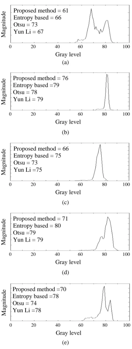
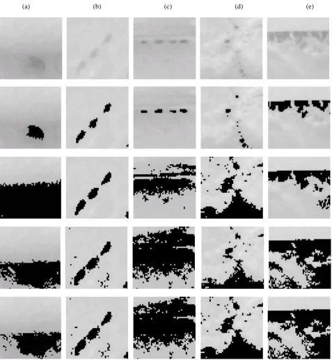
From Figure 9, it shows that our method provides the best result in segmenting all the test samples compare to other methods. However, when there is an even light concentration (Figure 9(b)), all the methods gave acceptable results. For uneven light concentration and complex background images (Figure 9(c), 9(d) & 9(e)), the results are contrary for Entropy based method, Yun Li method and Otsu method. Entropy based method and Yun Li method resulted in poor segmentation because false edges form from the uneven light concentration and complex background are also computed in their algorithms. As for the Otsu method, the poor segmentation is due to the object (defect) and the background does not separate well in the image histogram. Otsu method assumes that images have two normal distributions with similar variances. The threshold value is selected by separating the image histogram into two classes such that its inter-class variance is maximized [21]. Unfortunately, the uneven light concentration and complex background of the tested images cause the defects to become invisible in the Otsu computation. For the five images in Figure 9, the image histogram separation by Otsu method is shown in Figure 8. The figure also shows the threshold value for our method, the entropy based method and Yun Li method.
For image with the uneven light concentration but without the complex background (Figure 9(a)), Otsu method recognized the darker side as object although it is not the defect because the edges of the defects are very fuzzy where it can not be recognize in the image histogram. The entropy based method and Yun Li method segments the image better as they have edge element in their computation. For our method, where more flexibility for edge definition is included, defect image with fuzzy edges can be segmented properly.
VI. CONCLUSION
In this paper, a thresholding technique has been proposed based on the gray level co-occurrence matrix. The technique extracts the edge information and the gray level transition frequency from the GLCM to compute the threshold value. The algorithm is also designed to have the flexibility over the edge definition. Thus, it can handle image with fuzzy boundaries between the image’s object and background. The proposed technique was tested with starfruit defect image and result good segmentation in order to identify the area of the defect on the starfruit skin. The results were compared with three other techniques. It showed that segmentation using the proposed method gives the best result compared to the other method.
(a)
(b)
(c)
(d)
(e)
Figure 8. Image histogram and threshold value, (a) to (e) are plotted from image (a) to (e) in Figure 9 respectively.
REFERENCES
[1] A. Shio, “An Automatic Thresholding Algorithm Based On An Illumination-Independent Contrast Measure”, IEEE
Computer Society Conference on Computer Vision and Pattern Recognition, pp. 632-637, 4-8 June 1989.
Proposed method = 61 Entropy based = 66 Otsu = 73
Yun Li = 67
0 20 40 60 80 100
Gray level
Magni
tude
Proposed method = 76 Entropy based =79 Otsu = 78
Yun Li = 79
0 20 40 60 80 100
Gray level
Magni
tude
Proposed method = 66 Entropy based = 75 Otsu = 73
Yun Li =75
0 20 40 60 80 100
Gray level
Magni
tude
Proposed method = 71 Entropy based = 80 Otsu =79
Yun Li = 79
0 20 40 60 80 100
Gray level
Magni
tude
Proposed method =70 Entropy based =78 Otsu = 74
Yun Li =78
0 20 40 60 80 100
Gray level
Magni
[2] N. Otsu, “A Threshold Selection Method from Gray-Level Histogram”, IEEE Trans. on System Man Cybernetics, SMC, vol. 9(I), pp. 62-66, 1979.
[3] J. Kittler and J. Illingworth. “Minimum Error Thresholding”, IEEE Transactions on Pattern Recognition, vol. 19, No.1, pp. 41-47, 1986.
[4] M. Takatoo, “Gray scale Image Processing Technology Applied to Vehicle Licence Number Recognition System”, Proceeding of Int. Workshop on Industrial Applications of Machine Vision and Machine Intelligence, pp 76-79, 1987.
[5] F.H.Y. Chan, F.K. Lam, Hui Zhu, “Adaptive Thresholding By Variational Method”, IEEE Transactions on Image
Processing, vol. 7, no. 3, pp. 468-473, March 1998.
[6] D. L. Milgram, “Region Extraction Using Convergent Evidence”, IEEE Trans. on Computer Graphics and Image Processing, vol. 11 no. 1, 1979.
[7] S. D. Yanowitz and A. M. Bruckstein, “A New Method For Image Segmentation”, IEEE Trans. on Computer. Vision, Graphic and Image Processing, vol. 46, pp. 82-95, 1989.
[8] Zhonghua liu and Qilong Wang, “Edge Detection And Automatic Threshold Based On Wavelet Transform In The VPPAW Keyhole Image Processing”, IEEE Conference Record of the Industry Applications Conference, vol. 2, pp. 1048-1053, 8-12 Oct. 2000.
[9] Xiao-Ping Zhang and M.D. Desai, “Segmentation Of Bright Targets Using Wavelets And Adaptive Thresholding”, IEEE Transactions on Image Processing, vol. 10 no. 7, pp. 1020-1030, July 2001.
[10] M.L.G. Althouse, C.I. Chang, “Image Segmentation By Local Entropy Methods”, Proceedings of the International Conference on Image Processing, vol. 3, pp. 61-64, 1995.
[11] Y. Ebrahim, “Entropy based thresholding of cross-dissolved ultrasound images”, Canadian Conference on
Electrical and Computer Engineering, vol. 3. pp. 1477-1480, 2003.
[12] Shung-Shing Lee, Shi-Jinn Horng, Horng-Ren Tsai, “Entropy Thresholding And Its Parallel Algorithm On The Reconfigurable Array Of Processors With Wider Bus Networks”, IEEE Transactions on Image Processing, vol. 8 no. 9, pp. 1229-1242, Sept. 1999.
[13] N.R. Pal and S.K. Pal, “Entropy Thresholding”, IEEE Trans. on Signal Processing, vol.16, pp. 97-108, 1989.
[14] C.I. Chang, K. Chen, J. Wang, M.L.G. Althouse, “A Relative Entropy-Based Approach To Image Thresholding”, IEEE Trans. on Pattern Recog., vol. 120, pp. 215-227, 1993.
[15] Yun Li, C. Mohamed, C.Y. Suen, “A Threshlod Selection Method Based On Multiscale And Graylevel Co-Occurrence Matrix Analysis”, Proc. of Eighth International Conference on Document Analysis and Recognition, vol. 2, pp. 575-578, 2005.
[16] J. Weszka, C. Dyer, A. Rosenfeld, “A Comparative Study Of Texture Measures For Terrain Classification”, IEEE Trans. on SMC, vol. 6, no. 4, pp. 269-285, April 1976.
[17] R.W. Conners, C.A. Harlow, “A Theoretical Comparison Of Texture Algorithms”, IEEE Trans. on PAMI, vol. 2, pp. 205-222, May 1980.
[18] A. Baraldi, F. Parmiggiani. “An Investigation Of The Textural Characteristics Associated With GLCM Matrix Statistical Parameters”, IEEE Trans. on Geoscience and Remote Sensing, vol. 33, no. 2, pp. 293-304, March 1995
[19] R. Haralick, K. Shanmugam, I. Dinstein, “Texture Features For Image Classification”, IEEE Transaction on SMC, vol. 3, no. 6, pp. 610-621, 1973.
[20] H. Tian, S.K. Lam, T. Srikanthan, “Implementing Otsu's Thresholding Process Using Area-Time Efficient Logarithmic Approximation Unit”, Proc. of the International Symposium on Circuits and Systems, vol. 4, pp. IV/21-IV/24, 25-28 May 2003.
[21] C.H. Chou, C.C. Huang, W.H. Lin, F. Chang, “Learning To Binarize Document Images Using A Decision Cascade”, IEEE International Conf. on Image Processing, vol. 2, pp. II/518-II/521, Sept. 2005.
[22] C.-I. Chang, Y. Du, J. Wang, S.-M. Guo, P.D. Thouin, “Survey and comparative analysis of entropy and relative entropy thresholding techniques”, IEE Proceedings-Vision, Image and Signal Processing, vol. 153, no. 6, pp. 837 - 850, Dec. 2006.
(a) (b) (c) (d) (e)