Nadi et al. World Journal of Engineering Research and Technology
SIMPLE SIMULATION MODEL FOR BIOLOGICAL DESALINATION
BY ALGAE
El Nadi M. H.*1, El Hosseiny O. M. 2 and Nasr N. A. H.3
1
Professor of Sanitary & Environmental Eng., Faculty of Eng., ASU, Cairo, Egypt.
2
Assistant Professor of Sanitary Eng., Civil Eng. Dept., CIC, New Cairo, Egypt.
3
Associate Professor of Sanitary Eng., Faculty of Eng., ASU, Cairo, Egypt.
Article Received on 04/12/2018 Article Revised on 25/12/2018 Article Accepted on 15/01/2019
ABSTRACT
The study was made to determine the mathematical model for the desalination reactor that depends on algae biological action. The equation proved to obtain removal efficiency of total dissolved solids from saline water by the means of the green algae Scenedesmus species through a continuous flow treatment system. Algae were added to two consecutive reactors in which a 7 days retention time was applied in each. The experiment in the continuous flow was repeated for 4 runs and the average values were taken into consideration. Physico-chemical analysis of growth media was daily determined. Total dissolved solids removal efficiencies measured in the output of both first and second reactors reached around 88% for each and 97% for the overall plant. The results were used to produce the simulated equation for the action taking into consideration the effective parameters. The equation verification was done with error range than field results + 10%. This shows the success of the equation to simulate the system which is a new promising technique to produce suitable potable water from sea water.
KEYWORDS: Water Desalination, Biological Desalination, Water Desalination by Algae, Simulation Modeling.
World Journal of Engineering Research and Technology
WJERT
www.wjert.org
SJIF Impact Factor: 5.218*Corresponding Author
El Nadi M. H.
INTRODUCTION
Green algae was used for treatment of industrial wastewater from natural gas production fields contains salinity up to 25000 ppm and oil content up to 100 ppm. The effluent could be reused in irrigation of crops with a flow enough for about 60 fed./day. While the produced algae 1.5 ton/day that could be used in medical industry, pigments for industry, functional food, bio-fertilizers, and animal or fish fodders.[1] In a pilot erected for industrial wastewater in N/D field in Abu-Mady north of Egypt using algae ponds the achieved removal efficiencies for TDS and high oil content was 90-95 % that proved the suitability of algae application for saline industrial wastewater treatment.[2]
Desalination based on the use of algae in the removal of salts from saline water, and water production for use in different purposes is a new concept and it was successfully used in industrial wastewater treatment. The achieved results were promising and good in the desalination of sea water and is successful, continuing to reach the removal efficiency up to 95% till the rates are relatively affordable for possible use in different purposes, opening the door to a new direction may succeed in solving the problem of water desalination with cost reduction to the minimum possible.[3]
Algae as a group exhibit an extremely wide range of tolerance to salts in their surroundings. As for the adaptation to salinity, Algae may be roughly divided into tolerant and halo-philic, the later requiring salt for optimum growth and the former having response mechanisms that permit their existence in saline medium.[4]
Micro-algae have a high capacity for inorganic nutrient uptake and can be used in mass culture in outdoor solar bioreactors. Unicellular green algae such as Chlorella and
Scendesmus have been widely used in wastewater treatment because they often colonize the ponds naturally, and they have fast growth rates and high nutrient uptake capabilities. However, one of the major drawbacks of using micro-algae in wastewater treatment is the harvesting of biomass.[5]
Different Models of Algae Ponds
Model No. (1)
D. Dochain et al.[6] developed a dynamical modeling of a waste stabilization pond and it is aimed at understanding the relations between descriptive aspects, and also to predict whenever there is a risk of odor and also to calibrate of the model parameters. The data were collected as follows: light intensity (measured at 3 m above the pond surface), air temperature, and dissolved oxygen and temperature at two different depths (–10 cm and – 30 cm) and the system was basically homogeneous all over the year.
Three microbial populations are considered: X1 (microalgae), X2 (aerobic bacteria), X3
(sulphate-reducing bacteria). The influent substrate is shared into soluble (S1) and insoluble material (S2). The lagoon is vertically stratified in two homogenous compartments, in the upper compartment (approximately 80 cm depth) the aerobic bacteria utilize the substrate S1 with dissolved oxygen, O2; in the lower compartment (i.e. the sediments, approximately
20 cm depth) the sulfate-reducing bacteria utilize the substrate S1 (Si=substrate in layer i [i=1,2]). Dead biomass in both compartments enriches substrate S2. The hydrogen sulfide (H2S) produced by the sulfate-reducing bacteria was oxidized by the dissolved oxygen in the
upper compartment. H2S is also considered as an inhibitor of the sulfate-reducing bacteria
and of the microalgae.[6]
The microalgae growth is a function of light with a "delay" effect (algae may still produce oxygen for some time after sunset). The dynamical mass balance equations.[7] illustrate that the specific growth rate of microalgae is inhibited by the hydrogen sulfide presence and is directly driven by the insulation term taking into account the light dependence and the photoinhibition of microalgae.
(1)
(2)
where µ1,max, K1, Ki1 are the maximum specific growth rate of the microalgae growth, the
saturation constant for S1 and the inhibition coefficient for H2S, respectively. is the mean
The microalgae death is known to depend on the dissolved concentration O2 as follows:
(3)
Where m1,max and KO the maximum death coefficient of the microalgae and the inhibition
constant for the oxygen, respectively.
It has to be noted that the dissolved oxygen concentration actually increases with microalgae activity, which in turn depends of the light intensity and temperature. However, as expressed by equation (3), high light intensity inhibits the microalgae. Experimentally it was observed that the dissolved oxygen concentration was maximal in spring, autumn and somewhat lower during the hottest summer days.
Model No. (2)
Young chul Kim, Jaehong Park, Dimosthenis L. Giokas, and Triantafyllos A. Albanis[8] study Performance Evaluation and Mathematical Modeling of Nitrogen Reduction in Waste Stabilization Ponds. The aim of this study is to study the different combinations for nitrogen removal in configurations of shallow algal ponds (SAPs), SAPs followed by WSPs, water hyacinth ponds (WHPs) followed by WSPs, and WSPs treating secondary effluent from municipal wastewater treatment plant (WWTP) were investigated. Accordingly, a re-evaluation of the model of Reed,[9] in these systems was performed to study its application potential under various WSPs operating in series. Interestingly, based on the results obtained, a modification of the original model is proposed as means for the improvement of the prediction of nitrogen uptake from WSPs operating in series.
Based on extensive field experimental data, Reed developed the following semi-empirical nitrogen reduction model of WSPs in 1985.[10]
N/N0 =e{-k T(t+60.6(pH-6.6))} (4)
Equation (6) was derived from the ponds treating raw municipal wastewater. The original nitrogen model developed from the facultative WSPs operations was applied to the data obtained from the operation of shallow algal ponds (SAPs). The SAPs are similar to high-rate algal ponds in terms of shallow depth but with the exception that mechanical mixing is not provided. The application of the model to 22 individual data sets indicates that the predicted values correspond well with the measured values. The error range between calculated and measured values is 0.7–20.5% and the mean percentage error is about 5.8%.
The Reed model was tested to examine its utility when the pH difference between influent and effluent to and from the WSPs is very small, since two different types of algal ponds are operated in series.
The result of a total of 22 individual data points applied to the Reed model shows that it does not properly simulate the nitrogen concentrations of the effluent.[11]
It represents the treatment study of domestic wastewater by the WSPs following pretreatment of the raw sewage by water hyacinth ponds.[8] The Reed’s model predicts the nitrogen concentrations very well within a wide range of concentration during the operational period.
Comparing the results of Cases II and III it is shown that successive treatment by aerobic ponds results in the deterioration of the performance of Reed’s model,[9]
while an initial anaerobic stage of treatment (water hyacinth ponds) does not interfere with its simulation efficiency. This behavior can be attributed to the type and quality of wastewater. Initial treatment by anaerobic pond normally decreases difficult oxidized species more efficiently than readily oxidized,[12,13] This means that influent to the WSPs from WHPs contains a significant fraction of readily bioavailable substrate, which is efficiently utilized by aerobic bacteria.
lying somewhere in the middle of all of the above cases (lower than Cases I and III and higher than Case II).[8] The results reveal that the Reed’s model provided a reasonable description of nitrogen concentration profiles.
Model No. (3)
H. Jupsin,[14] evaluated a dynamic mathematical model of high rate algal ponds (HRAP) compatible with the Activated Sludge Model 1 (ASM1) and River Water Quality Model 1 (RWQM1) for rivers. The biochemical processes are based on elemental mass balances. The hydrodynamics of the system are modeled by a series of completely mixed reactors with recirculation. The biochemical processes parameters are taken from the RWQM1 model and the hydrodynamic parameters will depend on the geometry of the reactor & the mixing equipment (paddle wheel, air-lift, etc.).
As this model seeking to develop description of the sediment activity, So far this activity is taken into account by an equation that is dependent on the substrate concentration and temperature:
R = [Ro + Rmax
S KS
S
] θ
t-20
(5)
Where R: sediment respiration rate (g O2 m–2 day–1), R0: endogenous respiration rate (g O2 m– 2
day–1), Rmax: maximum respiration rate related to substrate (g O2 m–2 day–1), S: substrate
concentration (mg COD l–1) & KS: Michaelis constant (mg COD l–1).
As the main biochemical processes such as photosynthesis are highly dependent on weather conditions, that HRAP performance variables should be related to local conditions. For this reason the light intensity is calculated by a subroutine developed in the TRNSYS package.[15]
It must be said that the calculation process does not take into account the meteorological conditions, the weather is assumed to be fine and the sky cloudless. Finally, allowing for the self-shading of the algae and biomass:
η = 0.32 + 0.03*(Suspended solids) (6)
Ieff =
depth
0
Where:
Depth: total depth of the pond (m), Isurf: light intensity at the pond’s surface (W/m2), Ieff: total
light intensity in a vertical slice of the pond (W/m2), z: distance from the surface (m) & dz: calculation step (m)
Model No. (4)
Fergalla, et al,[16] produced the following modeling equations for the algae desalination ponds using the trend lines for the field results and the algae growth equation as follows:
Case 1 For TDS R.E. % for TDS above 20000 ppm:
TDS R.E. = -2816.5 (KTθ (Current Temperature – 20 Cº)) 3+916.68 (KTθ (Current Temperature – 20 Cº)) 2 + 219.8 (KTθ (Current Temperature – 20 Cº)
)+ 8.4806 ... (8)
Case 2 For TDS R.E. % for TDS between 20000 & 1000 ppm
TDS R.E. = -201.33 (KTθ (Current Temperature – 20 Cº)) 3 -293.2 (KTθ (Current Temperature – 20 Cº)) 2 + 302.37 (KTθ (Current Temperature – 20 Cº)
) + 3.649... (9)
Case 3 For TDS R.E. % for TDS below 1000 ppm TDS R.E. = 260.3 (KTθ (Current Temperature – 20 Cº)
) 3 -245.1 (KTθ (Current Temperature – 20 Cº)) 2 + 147.35 (KTθ (Current Temperature – 20 Cº)
) + 0.3406 ... (10)
Where:
K is a variable affected by TDS concentration and simulate the sunlight period and temperature, T is the period inside the basin and Ө is constant = 1.066 under 20°C
K can be calculated from the following equation
SLT = –139828 K2 + 6772.4 K – 69.325 ...(11)
Where:
SLT is the sunlight time factor = SL * TF……….(12)
& SL is the Sunlight exposing time in hours andTF is the ratio between current temperature and optimal temperature for Algae growth (27.5 Celsius).
MATERIALS AND METHODS
A pilot plant was designed as a continuous flow system to study the TDS uptake by the green algae. The optimum retention time and composed growth medium which gave the highest efficiency in minerals removal through the batch experiment were applied in this pilot plant. The experiment in the continuous flow lab scale pilot was repeated for 4 runs and the average values were taken into consideration. The continous flow lab scale system is shown in figure (1).
The green algae Scenedesmus sp. was used in the current investigation. Cultures were early grown under conditions of BG-11 growth medium.[17] As growth reached the maximum, cultures were harvested and washed three times to remove all surface-accompanied nutrients then cells were centrifuged at 5000rpm, and the algal bulk was used for treatment. The optimum retention time was taken 7 days as determined by El Nadi et al.,[3] from a batch scale experiment.
Samples were withdrawn from tanks everyday through 7 days, water analysis on the effluent was run where measurements were TDS, NO3, PO4, Cl2, Na, and SO4. The operation schedule
was as shown in table 1.
RESULTS
Several experiments had been performed to obtain the effect of algae application for the optimum retention time on different water quality parameters.
After providing a contact between the algae and the flow for 7 days in the first reactor, the effluent had a TDS value of 7500 ppm which was much higher than the target. The flow was introduced to another reactor as a secondary treatment or second treatment stage identical to the first one with the same design criteria to increase the removal efficiency to be nearer to the target. The experiment in the continuous flow was repeated for 4 parallel runs for each stage and the average values were taken into consideration for the first type of reactors and for the second type as well.
The application of the proposed system with the optimum design parameters was done on two successive reactors of continuous flow, each reactor of retention time 7 days to avoid algae decay and enzymes execration, with centrifugation before application on the second reactor then adding new fresh algae.
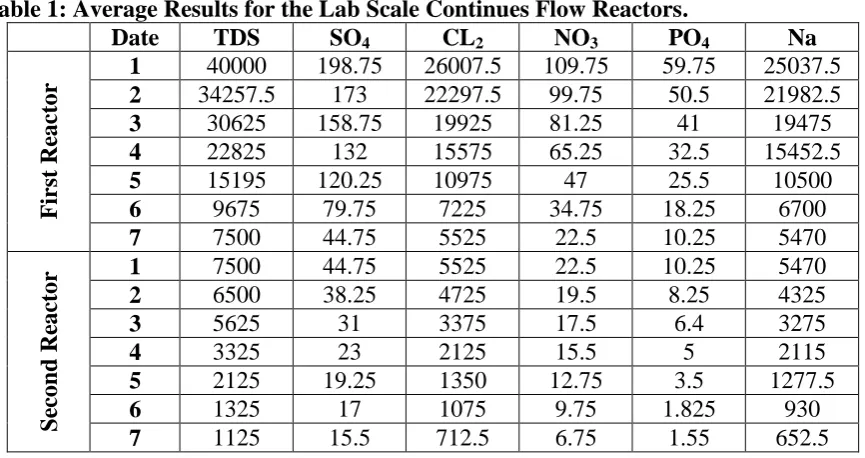
The measurements of different parameters through the continuous flow experiments are illustrated in table (1).
Table 1: Average Results for the Lab Scale Continues Flow Reactors.
Date TDS SO4 CL2 NO3 PO4 Na
First
Re
ac
tor
1 40000 198.75 26007.5 109.75 59.75 25037.5
2 34257.5 173 22297.5 99.75 50.5 21982.5
3 30625 158.75 19925 81.25 41 19475
4 22825 132 15575 65.25 32.5 15452.5
5 15195 120.25 10975 47 25.5 10500
6 9675 79.75 7225 34.75 18.25 6700
7 7500 44.75 5525 22.5 10.25 5470
S
ec
on
d
Re
ac
tor
1 7500 44.75 5525 22.5 10.25 5470
2 6500 38.25 4725 19.5 8.25 4325
3 5625 31 3375 17.5 6.4 3275
4 3325 23 2125 15.5 5 2115
5 2125 19.25 1350 12.75 3.5 1277.5
6 1325 17 1075 9.75 1.825 930
Model Design
The design of the model was performed after studying the previous models that mainly available for algae growth rate with temperature and sunlight intensity.
Based on the study of the previous models and the parameter measured it was found that the main effective parameters in the removal of the total dissolved solids (TDS) using algae is the algae growth rate and the detention time of the algae in the process. Our study selected the main effective parameters on the algae growth and desalination process with putting the temperature constant using its optimal value for algae growth to insure the effect of the other parameters and get the relation with TDS consumption that is the main study target. The relation between the effective parameters that obtained was studied with the relation between algae growth rate and both temperature and time from previous studies helps in producing the design modeling equation. The main target to achieve an equation simulate the real data with correlation coefficient more than 0.95. Here after the study illustrates the modeling production procedure and the steps made to obtain the design equation of the system explaining all the factors affecting the TDS consumption by algae and the methodology of their effect on the produced equation.
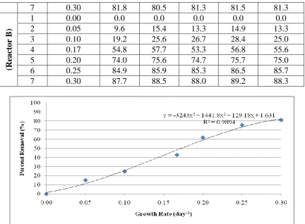
Using the experimental work data, relations between TDS removal ratio and both of algae growth rate and time period could be determined. To obtain the modeling equation, the relation between the average algae growth rate and the average percent removals of the TDS obtained from the four runs in the continuous flow stages versus the algae growth rate and time were studied and plotted. The data is presented in table (2), taking into consideration that the flow from reactor B was obtained from reactor A. The equations connected the average TDS percent removal versus the algae growth rate are obtained by plotting curves and add trend lines between the various parameters. The curves and equations are presented in the figures (2) and (3).
Table 2: Average Growth rate and TDS Removal Ratio. Time
(days)
Growth rate (day-1)
Removal R1%
Removal R2%
Removal R3%
Removal R4%
Removal Average% (R eac tor A
) 1 0.00 0.0 0.0 0.0 0.0 0.0
7 0.30 81.8 80.5 81.3 81.5 81.3
(R
eac
tor
B
)
1 0.00 0.0 0.0 0.0 0.0 0.0 2 0.05 9.6 15.4 13.3 14.9 13.3 3 0.10 19.2 25.6 26.7 28.4 25.0 4 0.17 54.8 57.7 53.3 56.8 55.6 5 0.20 74.0 75.6 74.7 75.7 75.0 6 0.25 84.9 85.9 85.3 86.5 85.7 7 0.30 87.7 88.5 88.0 89.2 88.3
Figure 2: Relation between TDS Removal Ratio versus the Algae Growth Rate (Reactor A).
y = -7367.7x3 + 3071.6x2 + 32.572x + 1.2339
R2 = 0.995
0 10 20 30 40 50 60 70 80 90 100
0.00 0.05 0.10 0.15 0.20 0.25 0.30
Growth Rate (day-1)
Pe
rc
en
t
R
em
o
v
a
l
(%)
Figure 3: Relation between TDS Removal Ratio versus the Algae Growth Rate (Reactor B).
TDS R.R(%) = -3243(GR)3 + 1441.8(GR)2 + 129.18(GR) + 1.631 (13) With R² = 0.9894
The equation for the second reactor is
TDS R.R(%) = -7367.7(GR3)+3071.6(GR2) + 32.572 (GR) +1.2339 (14) With R² = 0.995
Temperature effects on the algal growth rate were related directly to maximum oxygen production rate. Algal growth rate, expressed as photosynthetic demand of carbon, was adjusted for temperature using the equation.[18]
Algae Growth Rate = θ (Temperature(C) - 20(C)
(15)
Typical θ values were reported to range between 1.01 and 1.2.[19]
also, it was reported as 1.066.[17] This equation was studied and the condition of the data from the experimental work was considered to establish the final equation representing the algae growth rate connected with time and temperature effect as follows:
GR =KT θ (Temperature(C) – 20(C) ………..….(16)
where: GR: growth rate (day-1), T: the duration time (days), K: variable related the time and exposing to sunlight during the day & θ: constant =1.066
The value of temperature was fixed to be 30oC during the period of the experiment and the values of K were obtained to be as presented in table (3)
Model Analysis
Table 3: Calculated TDS Removal ratio.
Reactor Time (days)
Algae Growth rate
TDS % Removal (equation) Accumulative% Removal (equation) Re ac to r A
1 0.00 1.40 1.4
2 0.05 10.42 10.4
3 0.10 26.75 26.8
4 0.17 53.01 53.0
5 0.20 65.40 65.4
6 0.25 79.77 79.8
7 0.30 85.53 85.5
Re
ac
to
r B
1 0.00 1.40 81.5
2 0.05 10.42 83.2
3 0.10 26.75 86.3
4 0.17 53.01 91.2
5 0.20 65.40 93.5
6 0.25 79.77 96.2
7 0.30 85.53 97.3
Study the overall removal ratio for the whole system shows that the accumulation of the both reactors achieved in total a higher removal ratio (as a number) than what obtained from each one alone, this was due to the calculated removal ratio for the second reactor were proportioned to the influent of the first reactor that illustrated such higher results.
Model Verification
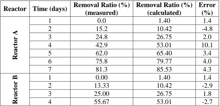
The results obtained from the equation were validated by calculating the error between the experimental work data and the calculated data from the equation to examine the accuracy of the equation and the deviation in its results than the actual measured results from the field as shown in tables (4) & (5).
Table 4: The Measured and Calculated TDS R.R (%) for each Reactor.
Reactor Time (days) Removal Ratio (%) (measured)
Removal Ratio (%) (calculated) Error (%) Re ac to r A
1 0.0 1.40 1.4
2 15.2 10.42 -4.8
3 24.8 26.75 2.0
4 42.9 53.01 10.1
5 62.0 65.40 3.4
6 75.8 79.77 4.0
7 81.3 85.53 4.3
Re
ac
to
r B 1 0.00 1.40 1.4
2 13.33 10.42 -2.9
3 25.00 26.75 1.8
5 75.00 65.40 -9.6 6 85.67 79.77 -5.9 7 88.33 85.53 -2.8
Table 5: The Measured and Calculated TDS R.R (%) of the System. Time
(days)
Removal Ratio (%) (measured)
Removal Ratio (%) (calculated)
Error (%)
1 0.0 1.4 1.4
2 15.2 10.4 -4.8
3 24.8 26.8 2.0
4 42.9 53.0 10.1
5 62.0 65.4 3.4
6 75.8 79.8 4.0
7 81.3 85.5 4.3
8 81.3 81.5 0.3
9 83.8 83.2 -0.5
10 85.9 86.3 0.3
11 91.7 91.2 -0.5 12 95.3 93.5 -1.8 13 97.3 96.2 -1.1 14 97.8 97.3 -0.5
Tables (4) and (5) show the variation between the measured & Calculated TDS removal ratio presenting the error between them which with in the range + 10 % that in the scientific research could be acceptable. Also in the engineering design this error can be covered by the design safety factors that should be taken to cover the unapplied parameters in the equation produced and the variations of the nature parameters as temperature and sunlight intensity.
The values of deviation ranged from - 9.6% to +10.1% which proved the equation suitability to simulate the system in the two reactors and shows the possibility to apply this equation for the system design for the low difference appeared from the results.
Figure 4: Comparison of Measure and Calculated TDS Removal Ratio in Reactor A.
Figure 5: Comparison of Measure and Calculated TDS Removal Ratio in Reactor B.
The previous figures Illustrated that in all cases the equation results was inside the margins + 10 % of the experiments results for removal ratio of TDS which insure the suitability of the application of the obtained equation to simulate the system and to be applicable as a design tool for such system. Also the figures and tables show the conversion of the start and end points for the system between equation and experiment results that are the most important values needed for design.
CONCLUSION
The main target of this study is to discuss and evaluate the applicability of a proposed new technique of algae ponds for desalination and determine its simulating equation for the system design. The biological desalination technique as a new one was proposed for its low capital and running cost compared with other desalination techniques. Green algae of
Scendesmus species was chosen in the suggested biological desalination for its high salinity tolerance. Generally, results encourage the use of green algae for desalination.
The results of this study had shown the following specific
conclusions:-1. The study determines Simple design simulation equation for the system applied for each reactor as follows:
% Removal TDS = - 5305.35 (K3T3θ(t-20)3) + 2256.7 (K2T2θ(t-20)2) + 80.876 (K*T* θ(t-20)) + 1.43245
Where GR: growth rate (day-1), T: the duration time (days).
K: variable related the time and exposing to sunlight during the day
θ: constant =1.066.
2. The determined design simulation equation achieved accuracy for TDS removal ratios of range + 10 % than the actual measured results which in the scientific research could be acceptable.
3. The values of deviation ranged from - 9.6% to +10.1% which proved the equation suitability to simulate the system in the two reactors and shows the possibility to apply this equation for the system design for the low difference appeared from the results. 4. The produced equation simulating the system under laboratory conditions (fixed
REFERENCES
1. Ibrahim, M.S., "Reuse and Recycle of Wastewater in Natural Gas Industry.", PhD Thesis, Inst. Of Environmental Studies & Researchs, ASU, Cairo, Egypt, 2005.
2. El Nadi, M. H., El Sergany, F.A. R & Ibrahim, M.S.M., "Use of Algae for Wastewater Treatment In Natural Gas Industry.", ASU, Faculty of Engineering Scientific Bulliton, Cairo, Egypt, September 2008; 1: 1687-1695.
3. El Nadi, M. H., El Sergany, F.A. GH. R "Water Desalination by Algea", ASU Journal of Civil Engineering, September 2010; 2: 105-114.
4. Gimmler, G., ‖The Metabolic Response of the Halotolerant Green Alga Dunalella parva to Hypertonic Shocks.‖ Ber. Deutsch.Bot. Ges. Bd., Gottingen, 1981; 94.
5. G, Laliberte; P, Lessard; J, De la Noue; S, Sylvestre, ―Effect of Phosphorus Addition on Nutrient Removal from Wastewater with the Cyanobacterium Phprmidium bohneri.‖
Bioresource Technology, 1997; 59: 227-233.
6. D. Dochain, S. Grégoire, A. Pauss and M. Schaegger "Dynamical modelling of a waste stabilisation pond" Bioprocess Biosystems Engineering, August 2003; 26(1): 19-26. 7. Bonvillain C, Benyamina D, Schaegger M, Pauss A,Bernard O, Dochain D"Modeling of
an extensive wastewater treatment plant lagoon", Conference on Advanced Wastewater Treatment ,Recycling and Conclusions Reuse,1416,Milan (Italy), September 1998; 1. 8. Kim, Youngchul, Park, Jaehong, Giokas, Dimosthenis L. and Albanis, Triantafyllos
A"Performance Evaluation and Mathematical Modeling of Nitrogen Reduction in Waste Stabilization Ponds in Conjunction with Other Treatment Systems", Journal of Environmental Science and Health, Part A, 2005; 39(3): 741 — 758.
9. Reed, S.C. "Nitrogen removal in wastewater stabilization ponds". Journal WPCF, 1985; 57(1): 39–45.
10.Oswald, W.J. "Introduction of advanced integrated wastewater ponding system". Water Sci. Technol., 1991; 24(5): 107.
11.Pinney, M.L.; Westerhoff, P.K.; Baker, L.A. "Transformations of dissolved organic carbon through a constructed wetland". Water Res., 2000; 34(6): 1897–1912.
12.Papadopoulos, A.; Parissopoulos, G.; Papadopoulos, F.; Karteris, A. "Variations of COD/BOD5 Ratio at Different Units Of a Wastewater Stabilization Pond Pilot Treatment
Facility", Proc. of the 7th International Conference on Environmental Science and Technology. Hermoupolis Syros; C369–C376, September 2001.
Applications in Mediterranean Countries". Proc. of the IWA Regional Symposium on Water Recycling in the Mediterranean Region. Iraklio, Greece, 327–336, September, 2002.
14.H. Jupsin, E. Praet and J.-L. Vasel "Dynamic mathematical model of high rate algal ponds". Water Science and Technology Vol 48 No 2 pp 197–204 IWA Publishing, 2003. 15.TRANSYS 15 (2000). "A transient system simulation program". Solar Energy
Labroatory, University of Wisconsin-Madison, Volume I USA, March, 2000.
16.Fergala, M.A.A. , El Hosseiny, O.M. & El Nadi, M.H. A., “Simulation Model for
Biological Desalination with Algae Ponds under nature conditions.”, ICNEEE
Conference, Faculty of Engineering & Technology, Future University in Egypt, Cairo, Egypt, April, 2016; 11-14.
17.Stainer, R.Y., Kuinsawa, M.M., Cohen-Bazire, G., ―Purification and Properties of Unicellular Blue Green Algae.‖, Bacteriology, 1971; 35: 171-201.
18.Simonsen, J. F. and P. Harremoest "Oxygen and pH fluctuations in Rivers". Water Research, 1978; 12: 477-489.