R E S E A R C H
Open Access
Network-based data classification: combining
K
-associated optimal graphs and high-level
prediction
Murillo G Carneiro
1*, João LG Rosa
2, Alneu A Lopes
2and Liang Zhao
3Abstract
Background: Traditional data classification techniques usually divide the data space into sub-spaces, each representing a class. Such a division is carried out considering only physical attributes of the training data (e.g., distance, similarity, or distribution). This approach is called low-level classification. On the other hand, network or graph-based approach is able to capture spacial, functional, and topological relations among data, providing a so-called high-level classification. Usually, network-based algorithms consist of two steps: network construction and classification. Despite that complex network measures are employed in the classification to capture patterns of the input data, the network formation step is critical and is not well explored. Some of them, such asK-nearest neighbors algorithm (KNN) and-radius, consider strict local information of the data and, moreover, depend on some
parameters, which are not easy to be set.
Methods: We propose a network-based classification technique, named high-level classification on K-associated optimal graph (HL-KAOG), combining the K-associated optimal graph and high-level prediction. In this way, the network construction algorithm is non-parametric, and it considers both local and global information of the training data. In addition, since the proposed technique combines low-level and high-level terms, it classifies data not only by physical features but also by checking conformation of the test instance to formation pattern of each class
component. Computer simulations are conducted to assess the effectiveness of the proposed technique.
Results: The results show that a larger portion of the high-level term is required to get correct classification when there is a complex-formed and well-defined pattern in the data set. In this case, we also show that traditional classification algorithms are unable to identify those data patterns. Moreover, computer simulations on real-world data sets show that HL-KAOG and support vector machines provide similar results and they outperform well-known techniques, such as decision trees and K-nearest neighbors.
Conclusions: The proposed technique works with a very reduced number of parameters and it is able to obtain good predictive performance in comparison with traditional techniques. In addition, the combination of high level and low level algorithms based on network components can allow greater exploration of patterns in data sets.
Keywords: High-level classification; Complex network; Machine learning; Data classification
Background Introduction
Complex networks gather concepts from statistics, dynamical systems, and graph theory. Basically, they are large-scale graphs with nontrivial connection patterns [1]. In addition, the ability to capture spacial, functional, and
*Correspondence: [email protected]
1Faculty of Computing (FACOM), Federal University of Uberlândia (UFU), Avenida João Naves de Ávila, 2160, Bloco B, Uberlândia 38400-902, Brazil Full list of author information is available at the end of the article
topological relations is one of their salient characteristics. Nowadays, complex networks appear in many scenar-ios [2], such as social networks [3], biological networks [4], Internet and World Wide Web [5], electric energy networks [6], and classification and pattern recognition [7-11]. Thus, distinct fields of sciences, such as physics, mathematics, biology, computer science, and engineer-ing have contributed to the large advances in complex network study.
Data classification is an important task in machine learning. It is related to construct computer programs able to learn from labeled data sets and, subsequently, to predict unlabeled instances [12,13]. Due to the vast number of applications, many data classification tech-niques have been developed. Some of the well-known ones are decision trees [14,15], instance-based learning, e.g., theK-nearest neighbors algorithm (KNN) [16], arti-ficial neural networks [17], Naive-Bayes [18], and support vector machines (SVM) [19]. Nevertheless, most of them are highly dependent of appropriate parameter tunning. Examples include the confidence factor and the minimum number of cases to partition a set in C4.5 decision tree; the K value in KNN; the stop criterion, the number of neu-rons, the number of hidden layers, and others in artificial neural networks; and the soft margin, the kernel function, the kernel parameters, the stopping criterion, and others in SVM.
Complex networks have made considerable contribu-tions to machine learning study. However, most of the researches related to complex networks are applied to data clustering, dimensionality reduction and semi-supervised learning [20-22]. Recently, some network-based tech-niques have been proposed to solve supervised learn-ing problems, such as data classification [8,10,11,23,24]. The obtained results show that network-based techniques have advantages over traditional ones in many aspects, such as the ability to detect classes of different shapes, absence of parameters, and the ability to classify data according to pattern formation of the training data.
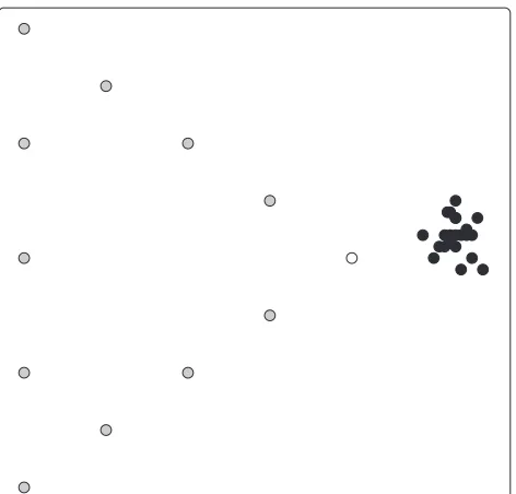
In [8], the authors proposed a network-based clas-sification algorithm, called K-associated optimal graph (KAOG). Among other characteristics, KAOG constructs a network through a local optimization structure based on a index of purity, which measures the compactness of the graph components. In the classification stage, KAOG combines the constructed network and a Bayes optimal classifier to compute the probability of a test instance belonging to each of the classes. One of the noticeable advantages of KAOG is that it is a non-parametric tech-nique. This is a desirable feature, which will be employed in the technique proposed in the present work. How-ever, both KAOG and other traditional classification tech-niques consider exclusively the physical features of the data (e.g., distance, similarity, or distribution). This lim-ited way to perform classification tasks is known as low-level classification [11]. However, the human (animal) brain performs both low and high orders of learning for identifying patterns according to the semantic meaning of the input data. Data classification that considers not only physical attributes but also the pattern formation is referred to as high-level classification [11]. Figure 1 shows an illustrative data set in which there are two classes (black and gray circles) and a new test instance to be classified
Figure 1A two-class data set, in which gray class data items form a triangle pattern.The white color instance needs to be classified in one of the classes.
(a white circle). Applying a SVM with optimized parame-ters and radial basis function as kernel, the test instance is classified into the black class. The same occurs when using optimized versions of another algorithms, such as KNN and decision tree. However, one could consider that the test instance belongs to the well-defined triangle pattern formed by the gray circles. This example shows that tradi-tional classification techniques fail to identify general data patterns. On the other hand, in [11], the authors present a quite different kind of classification technique that is able to consider the pattern formation of the training data by using the topological structure of the underlying network, which is called high-level classification. Specifi-cally, the data pattern is identified by using some complex network measures. The test instance is classified by check-ing its conformation to each class of the network. Again, considering Figure 1, the high-level technique is able to detect the pattern formed by gray cycle class and put the test instance into it. Furthermore, high-level and low-level classifications can work together in a unique framework, as proposed in [11].
In this paper, we propose a network-based classifica-tion technique combining two techniques: KAOG and the high-level classification. We referred to as high-level clas-sification onK-associated optimal graph (HL-KAOG). It considers not only the physical attributes but also the pattern formation of the data. Specifically, the proposed technique provides the following:
• A non-parametric way to construct the network • A high-level data classification with only one
parameter
• A more sensitive high-level classification by examining the network components instead of classes. This is relevant because classes can consist of several (eventually distinct) components. Thus, the components are smaller than the networks of whole classes. Consequently, the high-level tests are more sensitive and good results can be obtained
• An automatic way to obtain the influence coefficient for the network measures. In addition, this coefficient adapts itself according to each test instance
• A new complex network measure adapted to
high-level classification, named component efficiency
Computer simulations have been conducted to assess the effectiveness of the proposed technique. Interestingly, the results show that a larger portion of the high-level term is required to get correct classification when there is a complex-formed and well-defined pattern in the data set. In this case, we also show that traditional classifica-tion algorithms are unable to identify those data patterns. Moreover, computer simulations on real-world data sets show that HL-KAOG and support vector machines pro-vide similar results and they outperform well-known tech-niques, such as decision trees andK-nearest neighbors.
The remainder of the paper is organized as follows: A background and a brief overview about the related works are presented in the ‘Overview’ section The proposed technique and the contributions of this work are detailed in the ‘Methods’ section. Empirical evaluation and dis-cussions about the proposed algorithm on artificial and real data sets are showed in the ‘Results and discussion’ section. Finally, the ‘Conclusions’ section concludes the paper.
Overview
In this section, we review the most relevant classifi-cation techniques. Firstly, we present an overview on the network-based data classification. Then, we describe the network construction and classification using theK -associated optimal graph. Finally, we present the rationale behind the high-level classification technique.
Network-based data classification
In data classification, the algorithms receive as input a given training data set, denoted here X = {(inp1,
lab1),. . .,(inpn, labn)}, where the pair (inpi, labi) is the i-th data instance in the data set. Here, inpi=(x1,. . .,xd) represents the attributes of ad-dimensional data item and labi∈L= {L1,. . .,LC}represents the target class or label associated to that data item.
In network-based classification, the training data is usu-ally represented as a network in which each instance is a vertex and the edges (or links) represent the similarity relations between vertices. The goal of the training phase is to induce a classifier from inp → lab by using the training dataX.
In the prediction (classification) phase, the goal is to use the constructed classifier to predict new input instances unseen in training. So, there is a set of test instances Y = {(inpn+1, labn+1),. . .,(inpz, labz)}. In this phase, the algorithm receives only the inp and uses the constructed network to predict the correct class lab for that inp.
K-associated optimal graph
KAOG uses a purity measure to construct and optimize each component of the network. The resulting network together with the Bayes optimal classifier is used for clas-sification of new instances. Specifically, a KAOG is a final network merging severalK-associated graphs while main-taining or improving their purity measure. For the sake of clarity, the network construction phase can be divided in two concepts: creating aK-associated graph (Kac) and creating aK-associated optimal graph.
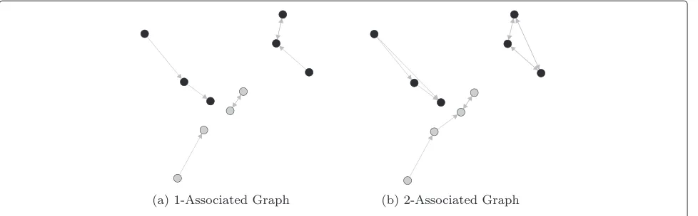
The K-associated graph builds up a network from a given data set and a K value, which is related to the number of neighbors to be considered for each vertex. Basically, the algorithm only connects a vertex vitovjifvj is one of theK-nearest neighbors ofviand ifviandvjhave the same class label.
Algorithm 1 shows in detail how aK-associated graph is constructed. In Kac,Vdenotes the set of verticesvi ∈V, which represents all training instances;Eprovides the set of edgesei,j∈E, which contains all links between vertices;
vi,K contains theK-nearest neighbors of vertexvi;ci is
Algorithm 1K-associated graph (Kac)
Require: Kand a data setX 1: for allvi∈Vdo
2: vi,K⇐ {vj|vj∈vi,Kandcj=ci}
3: E⇐E∪ {ei,j|vj∈vi,K}
4: end for
5: C⇐findComponents(V,E)
6: for allα∈Cdo
7: α⇐purity(α)
8: G(K)⇐G(K)∪ {(α(V,E); α)}
9: end for
the class label of vertexi; findComponents(V,E)is a func-tion that find all existing componentsa in the graph; C
is the set of all components α ∈ C;purity(α)gives the compactness α of each component α ∈ C; and G(K)
represents theK-associated graph. Figure 2 shows the for-mation of theK-associated graph for (a)K = 1 and (b) K=2.
Also, about the K-associated graph, there are two important characteristics that are highlighted as follows:
1. Asymmetrical property: according to Algorithm 1, Kac returns a digraph. Digraphs provide good representation for the asymmetric nature existing in many data sets because many timesvj∈vi,K does not implyvi∈vj,K.
2. Purity: this measure expresses the level of mixture of a component in relation to other components of distinct classes. Basically, the purity measure is given by
α =
Dα
2K, (1)
whereDαdenotes the average degree of a component
α; and2Kis the maximum number of possible links that a vertex can have.Dαcan be obtained by
Dα =
1 N
N
i=1
ki, (2)
in whichNis the total number of vertices inαandki is the degreebof vertexi.
Despite the fact thatK-associated graph presents good performance on data classification, there is a drawback: it uses the same value ofK to form networks for all data classes. However, rarely a network obtained by an unique value of K is able to produce the best configuration of instances in the components, in terms of the purity mea-sure. In this way, an algorithm, which is able to adapt itself to different classes of the data set is welcome. The idea of KAOG is to obtain the optimalK value for each component in order to maximize its purity [8].
Algorithm 2 shows in detail the construction of KAOG fromK-associated graphs. In the algorithm,G(Ot)denotes
theK-associated optimal graph and lastAvgDegree is the average degree of the network before incrementing the value of K; note that no parameter is introduced in the algorithm. In the following, we describe Algorithm 2. In the first lines,K starts with the value 1 and, thus, the 1-associated graph is considered as the optimal graph (Gopt) at this moment. After the initial setting, a loop starts to merge the subsequentK-associated graphs by increasing K, while improving the purity of the network encoun-tered so far, until the optimal network measured by the purity degree [8] is reached. Between lines 7 and 12, the
algorithm verifies for each component of theK-associated graph (Cβ(K)) whether the condition given by line eight is satisfied. In affirmative case, an operation to remove the components that composeC(βK)from the optimal graph is performed (line 9). In line 10, the new component is added to Gopt. At the end, the algorithm returns the obtained components with their respective values ofKand purities.
Algorithm 2K-associated optimal graph Require: data setX
1: K⇐1
2: G(Ot)⇐Kac(K,X) 3: repeat
4: lastAvgDegree⇐D(K) 5: K⇐K+1
6: G(K)⇐Kac(K,X) 7: for allC(βK)⊂G(K)do
8: if(βK)≥(αOt)for allCα(Ot)⊆C(βK)then
9: G(Ot)⇐G(Ot)− ∪C(Ot) α ⊆C(βK)
C(αOt)
10: G(Ot)⇐G(Ot)∪ {Cβ(K)} 11: end if
12: end for
13: untilD(K)−lastAvgDegree<D(K)/K 14: return K-associated optimal graphG(Ot)
About the time complexity of the KAOG network con-struction, given a training set with N instances and d attributes, the complexity for generating the correspond-ing distance matrix is N(N − 1) ∗d which yields the complexity order of O(N2). Another functions such as
find the graph components and compute the purity mea-sure of the graph components yield the complexity order ofO(N). Therefore, the time complexity to build up the network isO(N2)[8].
After the construction of the KAOG network, a Bayes optimal classifier (BayesOC) performs the classification of new instances using the constructed network. Let us con-sider a new instanceyto be classified. KAOG performs the classification computing the probability ofybelonging to each component. Thus, from the Bayes theory, thea pos-terioriprobability ofyto belong to a componentαtaking theKα-nearest neighbors of this new case (y) is given by
P(y∈α|y)=
P(y|y∈α)P(y∈α) P(y)
. (3)
According to [8], the probability of the neighborhoody given thatybelongs toαis given by
P(y|y∈α)= |
y,Kα∩α|
Kα
Figure 2Network formation usingK-associated graph algorithm.
The normalization termP(y)is obtained by
P(y)=
Ny,β=0
P(y|y∈α)P(y∈α). (5)
Also, thea prioriprobabilityP(y∈α)is given by
P(y∈α)= α
Ny,β=0
β
. (6)
In addition, if the number of components in the net-work is bigger than the number of classes in the data set, BayesOC sums up the probabilities associated to the each classj, as follows:
P(yj)=
α∈j
P(y∈α|y). (7)
At the end, BayesOC chooses the class with the largest a posterioriprobability.
About the time complexity, the BayesOC classification yields the complexity order ofO(N)that is related to the calculation of the distance matrix between the training set and the test case [8].
High-level classification
High-level prediction considers not only physical attributes but also global semantic characteristics of the data [11]. This is due to the use of complex network mea-sures, which are able to capture the pattern formation of the input data. The next sections provide more details about high-level classification.
Network construction As all other network-based learning techniques, here, the first step is the network construction from the vector-based input data. In fact, the way how the network is constructed influences to a large extent the classification results of the high-level predic-tion. In [11], the authors propose a network construction
method combining the -radius and KNN algorithms, which is given by
Net(i)=
−radius(inpi, labi), if|−radius(inpi, labi)|>K KNN(inpi, labi), otherwise
(8)
where KNN and -radius return, respectively, the set containing theK-nearest vertices of the same class of ver-tex i and the set of vertices of the same class of i, in which the distance fromiis smaller than. Note thatK and are user-controllable parameters. In addition, the algorithm connects the vertex i to other vertices using
-radius when the condition is satisfied and usingKNN, otherwise.
As shown in Equation 8, the network formation algo-rithm depends on some parameters. Different parameter values produce very distinct results. Moreover, the model selection of the parameters is time-consuming. For this reason, we propose a non-parametric network formation method based on the KAOG to work together with the high-level technique. The ‘Methods’ section describes our proposal.
Hybrid classification technique In [11], the authors propose a hybrid classification technique combining a low-level term and a high-level term, which is given by
My(J)=(1−λ)Py(J)+λHy(J). (9)
assortativity and clustering coefficient [1]) betweenyand the classJ. Finally,λ∈[0, 1] is a user-controllable variable and it defines a weight assigned to each produced classi-fication. Note thatλjust defines the contribution of low-and high-level classifications. For example, ifλ= 0, only low-level algorithm works.
The high-level classification of a new instanceyfor a given classJis given by
Hy(J)=
Z
u=1δ(u)[1−f
(J)
y (u)]
g∈L
Z
u=1δ(u)[1−f
(g)
y (u)]
, (10)
whereHy(J) ∈[0, 1],uis related to the network measures employed in the high-level algorithm,δ(u) ∈[0, 1],∀u ∈ {1,. . .,Z}is a user-controllable variable that indicates the influence of each network measure in the classification process andfy(J)(u)provides an answer whether the test instance y presents the same patterns of the class J or not, considering theu-th network measure applied. The denominator term is only for normalization. There is also a constraint aboutδ(u); (10) is valid only ifKu=1δ(u)=1.
Aboutfy(J)(u), it is given by
fy(J)(u)=Gy(J)(u)p(J), (11)
in which G(yJ)(u) ∈[0, 1] represents the variation that occurs in a complex network measure whenever a new instancey ∈ Y is inserted andp(J) ∈[0, 1] is the propor-tion of instances that belongs to the classJ.
Complex network measures In fact, complex network measures are used to provide a high-level analysis on the data [25]. So, when a new instanceyneeds to be classified, the technique computes the impact by inserting this new vertex for each class in an isolated way. Basically, the vari-ation of the results in network measures indicates which is the class thatybelongs to. In other words, if there is a little variation in the formation pattern of that class when connectingyto it, high-level prediction returns a big value indicating thatyis in conformity with this pattern. In the opposite, if there is a great variation when linking y to a class, it returns a small value denoting thatyis not in conformity with this pattern.
In [11], three network measures are employed to check the pattern formation of the input data: assortativity, average degree, and clustering coefficient [26]. A more detailed view about the network measures employed in HL-KAOG is provided in the next section.
Methods
Most machine learning algorithms perform the classi-fication exclusively based on physical attributes of the data. They are called low-level algorithms. One example
includes the BayesOC algorithm showed in the pre-vious section. On the other hand, complex network-based techniques provide a different kind of classification that is able to capture formation patterns in the data sets.
Actually, the principal drawback in the use of com-plex network measures for the data classification is the network formation. Some techniques have been largely used in the literature, such as KNN and -radius, but they depend on parameters. This means that the tech-nique is not able to detect information in the data, so different parameters produce very distinct results. In HL-KAOG, we exploit the KAOG ability to produce an efficient and nonparametric network to address this problem. In addition, other contributions are presented here.
This section describes the principal contributions of this investigation. The ‘Component efficiency measure’ section shows a new complex network measure for high-level classification: the component efficiency. The ‘Linking high-level prediction and KAOG algorithm’ section pro-vides details about how KAOG network and high-level classifier work together. The ‘High-level classification on network components’ section denotes an important conceptual modification in our high-level approach: plex network measures are employed on graph com-ponents. The ‘Non-parametric influence coefficient for the network measures’ section shows an automatic way to obtain the influence coefficient of the network measures. The ‘Complex network measures per com-ponent’ section provides the adaptation of the complex network measures to work on components instead of classes.
Component efficiency measure
The component efficiency measure quantifies the effi-ciency of the component in sending information between its vertices. The component efficiency is a new network measure incorporated into the high-level classification technique. Its development is motivated by the concept of efficiency of a network [27], which measures how efficient the network exchanges information. Once our high-level algorithm is based on the component level, we named our measure as component efficiency.
Initially, consider a vertexiin a componentα. The local efficiency ofiis given by
E(α)i = 1 Vi
j∈i
qij, (12)
We define the efficiency of a componentαas the average of the local efficiency of the nodes that belong toα. So, we have
E(α)= 1 Vα
Vα
i=1
Ei(α), (13)
in whichVαis the number of vertices in the componentα.
Linking high-level prediction and KAOG algorithm
We adapted the concepts ofK-associated optimal graph and high-level algorithm to permit that they work together. Firstly,K-associated optimal graph divides the network in components according to purity measure. Thus, the high-level technique proposed here considers components instead of classes. In addition, different from BayesOC that considers only those components in which at least one vertex belongs to the nearest neighbors of the test instance, the high-level algorithm employs com-plex network measures to examine if the insertion of the test instance in a component is in conformity with the formation pattern of that component.
Figure 1 shows an illustrative example in which the net-work topology cannot be detected by the original KAOG. So, if we employ KAOG directly to our model, it would not be able to classify the new instance into gray cycle class. Instead, it will be classified into black cycle class. On the other hand, our model permits the correct classification because it uses available information in each component constructed by KAOG in a different way.
Suppose a test instancey will be classified. The clas-sification stage of our network-based technique can be divided in two steps according to [23]:
1. Firstly, the proposed technique uses the component efficiency measure to verify what are the components whereycan be inserted. This information is
important especially because it considers the local features of the components and establishes a heuristic that excludes components that are not in conformity with the insertion ofyinto them.
In a more formal definition, let us consider a component
αand a setFrelated to the components in which the varia-tions of complex network measures will be computed. For each new instancey,Fyis given by
Fy⇐Fy∪ {α| mine(α)y ≤E(α)}, (14)
wheree(α)y denotes the local efficiency ofyto each vertex that belongs to componentα andE(α)is the component efficiency ofα.
2. The next step is the insertion ofyin eachα∈Fy. According to our technique,ymakes connections with each vertexi∈αfollowing the equation given by
αy⇐α∪ {i|ey(i)≤E(α)}, (15)
whereαyincludes componentαand the connections betweenyand their vertices,e(yi)is the local efficiency in exchanging information betweenyandi, and e(yi)≤E(α)is the condition to be satisfied to assure a link betweenyandi.
Note that ifFy= ∅in (14) (very unusual situation), the algorithm employs theKαvalue associated with each
com-ponentα∈and verifies that the vertices inαare one of theKα-nearest neighbors ofy. If there is at least one
ver-tex that satisfies this condition in componentα, then the complex network measures are applied to this component; otherwise,αis not considered in the classification phase.
High-level classification on network components
Once the network is obtained by KAOG, the high-level algorithm can be applied to classify new instances by checking the variation of complex network measures in each component before and after the insertion of the new instance. Thus, the proposed high-level technique works on the components instead of whole classes. This is an important feature introduced in this work. Since each class can encompass more than one component, each component is smaller or equal to the corresponding whole class. In this way, the insertion of a test instance can gen-erate more precise variations on the network measures. Consequently, it is easier to check the conformity of a test instance to the pattern formation of each class compo-nent. On the other hand, the previous work of high-level classification considers the network of a whole class of data items. In this case, the variations are weaker and sometimes it is difficult to distinguish the conformity lev-els of the test instance to each class. Therefore, taking (9), the high-level classification of a new instanceyfor a given componentα, is given by
My(αJ)=(1−λ)Py(αJ)+λHy(αJ). (16)
whereαJ denotes a componentα in which its instances belong to class J, Py(αJ) establishes the association pro-duced by a low-level classifier between the instance y and the componentα, andHy(αJ)points to an association produced by the high-level technique betweenyand the componentα. The general idea behindHy(αJ)is very sim-ple: (i) KAOG network finds a set of components based on the purity measure, (ii) high-level technique examines these components in relation to the insertion of a test instancey, and (iii) the probabilities for each component
Also aboutHy(α), it represents the compatibility of each componentαwith the new instanceyand is given by
Hy(αJ)=
Z
u=1δy(u)[ 1−fy(α)(u)]
g∈L
Z
u=1δy(u)[ 1−fy(g)(u)]
, (17)
in whichuis related to the network measures employed in the high-level algorithm,δy(u) ∈[0, 1],∀u∈ {1,. . .,Z} indicates the influence of each network measure in the classification process, and fy(α)(u) provides an answer whether the test instance y presents the same patterns of the component α or not, considering the u-th net-work measure. The denominator term in (17) is only for normalization. Details about δy(u) are provided in the ‘Non-parametric influence coefficient for the network measures’ section.
From (17), a simple modification is performed in (11) to obtain a high-level classification on components (α) instead classes (J). So, we have
fy(α)(u)= G
(α)
y (u)p(α)
α
G(α)y (u)p(α)
, (18)
where the denominator term in (18) is only for normal-ization andp(α)∈[0, 1] is the proportion of instances that
belong to the componentα.
Non-parametric influence coefficient for the network measures
Differently of the previous works, the high-level tech-nique proposed in this work is non-parametric not only at the network construction phase but also at the classi-fication phase. We have developed an automatic way for the weight assignment among the employed network mea-sures, i.e., the δ term in Equation 17 is determined by
δy(u)=
1−(max
α G (α)
y (u)−min
α G (α)
y (u))
K
u=1 1−(maxα G
(α)
y (u)−min
α G (α)
y (u)) ,
(19)
in which G(α)y (u) ∈[0, 1] represents the variation that occurs in a complex network measure whenever a new instancey ∈ Y is inserted. Therefore,δy(u)is based on the opposite of the difference between the biggest and the smallestu-th network measure variation on all com-ponents α. The idea of determining δy(u) in this way is to balance all the employed network measures in the decision process and not permit only one network mea-sure to dominate the classification decision. Note that this equation is valid only ifKu=1δy(u)=1.
Complex network measures per component
The complex network measures presented in the previ-ous section work on classes. Differently of the approach proposed in [11], the approach proposed in this work considers pattern formation per component. This fea-ture makes the algorithm more sensitive to the network measure variations. In addition, the components are con-structed regarding the purity measure, which gives more precise information about the data set.
In this section, we adapted assortativity and clustering coefficient to work on components. Also, as the time com-plexity of the high-level classification is directly related to the network measures employed, we present the complex-ity order of each measure.
Assortativity (G(yJ)(1))
The assortativity measure quantifies the tendency of con-nections between vertices [26] in a complex network. This measure analyzes whether a link occurs preferentially between vertices with similar degree or not. The assorta-tivity with regard to each componentα of the data set is given by
r(α)=
L−1 u∈UJ
iuku−[L−1 u∈UJ
1
2(iu+ku)]2
L−1
u∈UJ
1
2(i2u+ku2)−[L−1 u∈UJ
1
2(iu+ku)]2
(20)
wherer(α) ∈[−1, 1],Uα = {u: iu ∈α∧ku ∈α} encom-passes all the edges within the componentα,urepresents an edge, andiu,kuindicate the vertices at each end of the edgeu.
Therefore, the membership value of a test instancey∈ Ywith respect to the componentαis given by
G(α)y (1)= |r (α)
−r(α)|
u∈U|
r(u)−r(u)|. (21)
The assortativity measure yields the complexity order of O(|E| + |V|), where|E|and|V|denote, respectively, the number of edges and the number of vertices in the graph.
Clustering coefficient (G(yJ)(2))
Clustering coefficient is a measure that quantifies the degree to which local nodes in a network tend to clus-ter together [28]. The clusclus-tering coefficient with regard to each componentαof the data set is given by
CCi(α)= |eus| ki(ki−1)
, (22)
CC(α)= 1 Vα
Vα
i=1
CC(α)i , (23)
in whichCCi(α)∈[0, 1] andVαdenotes the number of
instancey∈ Ywith respect to the componentαis given by:
G(α)y (2)= |CC (α)
−CC(α)|
u∈U
|CC(u)−CC(u)|. (24)
The clustering coefficient measure yields the complexity order ofO(|V| ∗p2), where|V|andpdenote, respectively, the number of vertices in the graph and the average node degree.
Average degree (G(yJ)(3))
The average degree is a very simple measure. It quantifies, statistically, the average degree of the vertices in a compo-nent. The average degree with regard to each component
αis given by
k(α) = 1 Vα
Vα
i=1
ki(α), (25)
in whichk(α) ∈[0, 1] andVα denotes the number of
ver-tices in componentα. Regarding the membership value of a test instancey ∈ Y with respect to componentα, it is given by
G(α)y (3)= | k (α)
− k(α) |
u∈|
k(u) − k(u) |. (26)
The average degree measure yields the complexity order ofO(|V|), where|V|denotes the number of vertices in the graph.
Results and discussion
In this section, we present a set of computer simula-tions to assess the effectiveness of HL-KAOG technique. The ‘Experiments on artificial data sets’ section supplies results obtained on artificial data sets, which emphasize the key features of the HL-KAOG. The ‘Experiments on real data sets’ section provides simulations on real-world data sets, which highlight a great ability of HL-KAOG to perform data classification. Note that the Euclidean dis-tance is used as similarity measure in all the experiments.
Experiments on artificial data sets
Initially, we use some artificial data sets presenting strong patterns to evaluate the proposed technique. These exam-ples provide particular situations where low-level classi-fiers by themselves have trouble to correctly classify the data items in the test set. Thus, this section serves as a tool for better motivating the usage of the proposed model.
The first step of HL-KAOG is the construction of the KAOG network. Different from other techniques of network construction, KAOG is non-parametric and it builds up the network considering the purity mea-sure (1). In the second step, HL-KAOG employs the
hybrid low- and high-level techniques to classify the test instances. The low-level classification here uses Bayes optimal classifier (3) and the high-level term uses the complex network measures given by (17) to capture the pattern formation of each component. Finally, the general framework given by (16) combines low- and high-level techniques.
Triangle data set
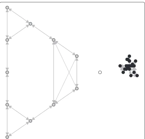
Figure 3 shows the KAOG network on a two-class data set. One can see that the gray class data items exhibit a strong pattern (similar to a triangle). Since the traditional machine learning techniques are not able to consider the pattern formation of classes, they cannot classify the new instancey(white color vertex) correctly. In addition, these techniques consider only the physical distance among the data items, which contributes to classifyyas belonging to class black. So, as the use of the Bayes optimal classifier, the same thing happens if we use other traditional tech-niques, such as decision tree,K-nearest neighbors, and support vector machine (SVM classifiers consider trans-formed feature space through a kernel function, but it is essentially based on the physical distance among the data), i.e., they are not able to identify the triangle pattern formed by the gray component.
Table 1 provides a detailed view about how the high-level classification is performed in HL-KAOG. Consid-ering the new instance y and the network showed in Figure 3, the classification process starts by computing each network measure on each component that satisfies (14). Then, HL-KAOG insertsytemporally in these com-ponents, according to (15), and computes the network
Table 1 Employed complex network measures in high-level classification on the Triangle data set
Cα Complex network measures
Assortativity Clustering coefficient Average degree
r(.) r(.) G(.)
y (1) f
(.)
y (1) CC(.) CC
(.)
G(y.)(2) fy(.)(2) E(.) E(.)
y G
(.)
y(3) f
(.) y (3)
Cgray 0.977 0.968 0.930 0.869 0.118 0.101 0.408 0.256 6.000 5.667 0.657 0.489
Cblack 0.850 0.851 0.070 0.131 0.188 0.212 0.592 0.744 8.000 7.826 0.343 0.511 The calculated assortativity, clustering coefficient, and component efficiency measures for each component.
measure on each of them again. So, the variation of each network measure before and after the insertion of the new instance can be obtained and (17) can be computed. Remember that the objective of the proposed function (19) is to balance the membership results obtained by the complex network measures in a way that the classifica-tion process is performed considering all of the applied network measures.
Table 2 presents the performance of the proposed tech-nique on the artificial data sets. The ‘Classification result’ column shows the final probability of classification when
λ = 0.2 andλ= 0.6 (high-level algorithms gets a higher contribution to the classification). The results showed in Table 2 emphasize some interesting properties of HL-KAOG. Firstly, one see that, combining a larger portion of the high-level classification (λ = 0.6), the technique is able to correctly classify the test instance when consider-ing a very clear pattern. However, usconsider-ing a larger portion of the KAOG classification (λ = 0.2), the pattern for-mation is not detected because Bayes optimal classifier considers only physical attributes to perform the predic-tion. Secondly, we employ a non-parametric technique to build up the network and to assign a weight to each
Table 2 Classification results (in terms of probability) obtained for each artificial data set whenλ=0.2 and λ=0.6
Data set Class Classification result
λ=0.2 λ=0.6
Triangle data set gray 0.439 0.516
black 0.561 0.483
Line I data set gray 0.481 0.586
black 0.519 0.414
Line II data set gray1 0.000 0.000
gray2 0.200 0.600
black1 0.400 0.200
black2 0.400 0.200
Multi-class data set black 0.800 0.400
gray 0.000 0.000
green 0.200 0.600
Italic values denote the final classification result.
network measure. So, HL-KAOG has only the λ value to set. Thirdly, HL-KAOG does not work on classes, but on the components. This is an important difference in relation to previous work about high level because the insertion of one vertex in a whole class of data items can seem very weak to present big network measures vari-ations. Thus, the variation at the component level can highlight better the variation when yis inserted in that component.
Line I data set
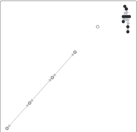
Figure 4 shows the KAOG network on a two-class data set, in which gray class presents a clear pattern of a straight line. Note that the three nearest neighbors of the new instanceybelong to the following classes: gray, black and black, respectively. In this way, KAOG classification is not able to detect the pattern presented by the gray com-ponent. The whole classification process performed by the Bayes optimal classifier on the KAOG is described as follows: Firstly, the algorithm computes the probability
a prioriof yto belong to each component as described in (6):
P(y∈Cgray)=0.5
P(y∈Cblack)=0.5
where the normalized purity measure of the components is used asa prioriprobability (gray=1 andblack =1).
Then, the probability of the neighborhoodygiven that y∈Cgrayandy∈Cblackis calculated as in(4):
P(y|y∈Cgray)=1/2
P(y|y∈Cblack)=2/3.
Then, the normalization term can be computed through (5):
P(y)≈0.583.
Finally, the final result of the KAOG classification on Line 1 data set can be obtained with (3) and (7):
Py(gray)=P(y∈Cgray|y)≈0.43 P(yblack)=P(y∈Cblack|y)≈0.57.
Note that other low-level algorithms classifyyas belong-ing to black class too. On the other hand, Table 2 shows that, with a high contribution of the high-level term (λ=
0.6), the technique can produce a correct label for y, according to the pattern formation presented in Figure 4.
Line II data set
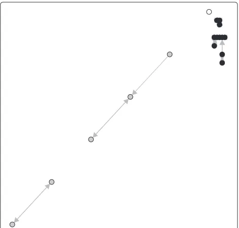
Figure 5 shows an interesting situation by two reasons. Firstly, because the new instance is very close to the black
Figure 5KAOG network generated from Line II data set.This data set is composed of two-class data items (gray and black). White data item needs to be classified.
components, it implies that the traditional techniques classify the new instance to the black class. Secondly, the big distances between the new instance and gray class data items make it difficult to be classified to the gray class. However, HL-KAOG can provide a correct classifi-cation due to its robustness to detect pattern formation, as shown in Table 2.
Multi-class data set
Figure 6 shows the KAOG network on a data set with three classes. There is a test instance (white color) that will be classified. Figure 6a presents a dubious case where there is no pattern formation related to the test instance. In this way, the technique (independent of theλ value) classifies the test instance as belonging to the black class. On the other hand, Figure 6b shows a more representa-tive information about the pattern formation related to the test instance. So, considering this clear pattern formation, the test instance is correctly classified when using a com-bination between low- and high-level algorithms where
λ=0.6 (Table 2).
Experiments on real data sets
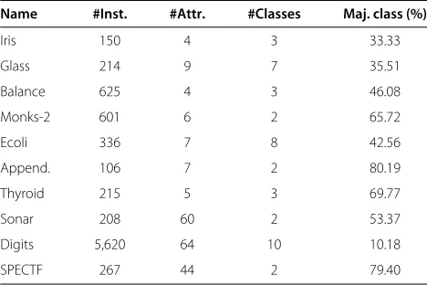
We also conducted simulations on real-world data sets available in UCI repository [29] and KEEL data sets [30]. Table 3 provides details about the data sets used here.
The proposed technique is compared to decision tree, K-nearest neighbors, and support vector machine. All these traditional techniques are available in the python machine learning module named scikit-learn [31]. Grid search algorithm is employed to perform parameter selec-tion for these techniques. For decision tree, scikit-learn provides an optimized version of the classification and regression tree (CART) algorithm [14]. In these exper-iments, two parameters are configured: the minimum density over the set {0,0.1,0.25,0.5,0.8,1}, which controls a trade-off in an optimization heuristic, and the mini-mum number of samples required to be at a leaf node, here denoted as ms, which is optimized over the set ms∈ {0,1,2,3, 4,5,10,15,20,30,50}. Based on the previous works applying the KNN on real-world data sets [8], aK value is optimized over the setK ∈{1,3,5,. . . ,31}, which is suf-ficient to provide the best results for this algorithm. In SVM simulations, we reduce the search space for the opti-mization process by fixing a single well-known kernel, namely the radial basis function (RBF) kernel. The stop-ping criterion for the optimization method is defined as the Karush-Kuhn-Tucker violation to be less than 10−3. For each data set, the model selection is performed by considering the kernel parameter γ ∈ {24, 23,. . ., 2−10
and the cost parameterC ∈ 212, 211,. . ., 2−2. Finally, the
Figure 6KAOG network found from different Multi-class data sets scenarious: (a) dubious case in detection of some pattern formation related to the test instance; (b) a clear pattern formation related to the test instance.
On the other hand, selection of parameters is unnec-essary for our technique when building up a network. Differently of the parameters in traditional machine learn-ing (such as K in KNN, kernel function in SVM, and so on),λvariable does not influence the training phase. In this way, we fixλ1=0.2 (due to good values found in [11])
andλ2=0.6 (to provide a very larger portion of the
high-level classification). In the previous section, artificial data sets provided particular situations where low-level tech-niques have trouble to perform the classification. Here, we evaluate (i) the linear combination betweenK-associated optimal graph and high-level algorithm, and (ii) the λ
influence in a context of real-world data sets. Once most techniques are essentially based on low-level character-istics, it is sure that these information contribute for a good classification. Consequently, when working together with low-level characteristics, high-level characteristics can improve the classification results by considering more than the physical attributes.
Table 3 Brief description of the data sets
Name #Inst. #Attr. #Classes Maj. class (%)
Iris 150 4 3 33.33
Glass 214 9 7 35.51
Balance 625 4 3 46.08
Monks-2 601 6 2 65.72
Ecoli 336 7 8 42.56
Append. 106 7 2 80.19
Thyroid 215 5 3 69.77
Sonar 208 60 2 53.37
Digits 5,620 64 10 10.18
SPECTF 267 44 2 79.40
Name, the data set name; #Inst., the number of instances; #Attr., the number of attributes; #Classes, the number of classes; Maj. class, the percentage of instances in the majority class.
Table 4 shows the predictive performance of the algo-rithms on real-world data sets presented in Table 3. In this table, ‘Acc’. denotes the average of accuracy for each technique and ‘Std.’ represents the standard deviation of this accuracies. In order to analyze statistically the results, we adopted a statistical test that compares multi-ple classifier over multimulti-ple data sets [32]. Firstly, Friedman test is calculated to check whether the performance of the classifiers are significantly different. Using a signif-icance level of 5%, the null hypothesis is rejected. This means that the algorithms under study are not equiva-lent. Following apost hoctest, Nemenyi test is employed (also considering a significance level of 5%). The results of this test indicate that HL-KAOG and SVM provide similar results and they outperform CART and KNN. This result is quite attractive because HL-KAOG, dif-ferent from other traditional techniques, is able to cap-ture spacial, functional, and topological relations in the data. In addition, the computer simulations show that a very larger portion of high-level classification (λ2) can
improve the final prediction in some real-world data sets. This means that these data sets present well-defined patterns, which can be detected considering mainly the topological structure of the data, instead of their physical attributes.
Conclusions
HL-KAOG takes advantages provided by theK-associated optimal graph and the high-level technique for data classification. Specifically, the former provides a non-parametric construction of the network based on the purity measure, while the latter is able to capture pattern formation of the training data. Thus, some contributions of HL-KAOG includes the following:
Table 4 Comparative results obtained by HL-KAOG, CART, KNN, and SVM on ten real-world data sets
HL-KAOG CART KNN SVM
Data set Acc.±Std. Acc.±Std. Acc.±Std. Acc.±Std.
Iris 97.33±3.52(λ1) 93.60±5.59 96.37±4.63 96.28±4.02
Glass 70.78±9.16 (λ1) 64.12±9.33 72.64±8.09 68.61±7.78
Balance 95.71±2.40 (λ1) 88.20±4.25 89.77±1.96 99.97±0.08
Monks-2 96.53±2.43(λ1) 95.67±2.48 81.26±5.02 93.79±3.22
Ecoli 84.90±5.73 (λ2) 80.78±5.55 85.99±5.11 87.23±5.22
Append. 83.54±7.27 (λ1) 77.24±9.95 86.99±8.71 85.72±8.15
Thyroid 97.30±3.16(λ1) 96.64±2.95 93.58±4.74 97.19±2.59
Sonar 83.75±8.07 (λ1) 74.14±9.69 81.78±8.08 86.06±7.43
Digits 98.75±0.35 (λ1) 90.27±1.27 98.79±0.37 99.26±0.33
SPECTF 80.07±5.42(λ2) 75.41±6.20 77.90±6.78 78.01±3.92
‘Acc’ and ‘Std’. denote, respectively, the average of accuracy and the standard deviation over 30 runs using the stratified 10-fold cross-validation process. In HL-KAOG, the classification result is obtained from the best value betweenλ1= 0.2 andλ2= 0.6. Italic values denote the best predictive performance among the techniques for
each data set.
test instance can generate bigger variations on the network measures. Consequently, it is much easier to check the conformation of a test instance to the pattern formation of each class component. On the other hand, the previous work of high level considers the network of a whole class of data items. In this case, the variations are very weak and sometimes it is difficult to distinguish the conformation levels of the test instance to each class.
• The use ofK-associated optimal graph to obtain a non-parametric network.
• An automatic way to obtain the influence coefficient for the network measures. In addition, this coefficient adapts itself according to each test instance.
• Development of a new network measure named component efficiency to perform the high-level classification.
Computer simulations and statistic tests show that HL-KAOG presents good performance on both artificial and real data sets. In comparison with traditional machine learning techniques, computer simulations on real-world data sets showed that HL-KAOG and support vector machines provide similar results and they outperform very well-known techniques, such as decision trees and K-nearest neighbors. On the other hand, experiments per-formed with artificial data sets emphasized some draw-backs of the traditional machine learning that, differently from HL-KAOG, are unable to consider the formation pattern of the data.
Forthcoming works include the incorporation of dynamical complex network measures, such as random walk and tourist walk, to the high-level classification algorithm, which can give a combined local and global vision in a natural way on the networks under analysis.
Future researches include also a complete analysis of the high-level classification when dealing with imbalanced data sets and the investigation of complex network mea-sures able to prevent the risk of overfitting in the data classification.
Endnotes
aA component is a sub-graphαwhere any vertices
vi∈Ccan be reached by othervj∈Cand cannot be reached by any other verticesvt∈/C.
bThe degree of a vertexv, denoted byk
v, is the total number of vertices adjacent tov.
Competing interests
The authors declare that they have no competing interests.
Authors’ contributions
MGC is the main author of this paper, which contains some results of his doctoral thesis in the Computer Science Program at Institute of Mathematics and Computer Science, University of São Paulo. MGC and LZ have contributed to the conceptual aspects of this work. Experiments and manuscript writing were performed by MGC under supervision of LZ, JLGR and AAL. All authors read and approved the final manuscript.
Acknowledgements
The authors would like to acknowledge the São Paulo State Research Foundation (FAPESP) and the Brazilian National Council for Scientific and Technological Development (CNPq) for the financial support given to this research.
Author details
1Faculty of Computing (FACOM), Federal University of Uberlândia (UFU),
Avenida João Naves de Ávila, 2160, Bloco B, Uberlândia 38400-902, Brazil.
2Institute of Mathematics and Computer Science (ICMC), University of São
Paulo (USP), Avenida Trabalhador São-Carlense, 400, São Carlos 13566-590, Brazil.3Department of Computing and Mathematics, School of Philosophy, Sciences and Literatures (FFCLRP), University of São Paulo (USP), Avenida Bandeirantes 3900, Monte Alegre, Ribeirão Preto, 14040-901, Brazil.
References
1. Newman M (2003) The structure and function of complex networks. SIAM Rev 45(2): 167–256
2. Costa LDF, Oliveira ON, Travieso G, Rodrigues FA, Boas PRV, Antiqueira L, Viana MP, Da Rocha LEC (2007) Analyzing and modeling real-world phenomena with complex networks: a survey of applications. Adv Phys 60(3): 103
3. Lu Z, Savas B, Tang W, Dhillon IS (2010) Supervised link prediction using multiple sources. In: 2010 IEEE international conference on data mining, Sidney, Australia, pp 923–928
4. Fortunato S (2010) Community detection in graphs. Phys Rep 486(3–5): 75–174
5. Boccaletti S, Ivanchenko M, Latora V, Pluchino A, Rapisarda A (2007) Detecting complex network modularity by dynamical clustering. Phys Rev Lett 75: 045102
6. Newman M (2010) Networks: an introduction. Oxford University Press, New York
7. Bertini JR, Lopes AA, Zhao L (2012) Partially labeled data stream classification with the semi-supervised k-associated graph. J Braz Comput Soc 18(4): 299–310
8. Bertini JR, Zhao L, Motta R, Lopes AA (2011) A nonparametric classification method based on k-associated graphs. Inf Sci 181(24): 5435–5456 9. Carneiro MG, Rosa JL, Lopes AA, Zhao L (2012) Classificação de alto nível
utilizando grafo k-associados ótimo. In: IV international workshop on web and text intelligence, Curitiba, Brazil, pp 1–10
10. Cupertino TH, Carneiro MG, Zhao L (2013) Dimensionality reduction with the k-associated optimal graph applied to image classification. In: 2013 IEEE international conference on imaging systems and techniques, Beijing, China, pp 366–371
11. Silva TC, Zhao L (2012) Network-based high level data classification. IEEE Trans Neural Netw 23: 954–970
12. Bishop CM (2006) Pattern recognition and machine learning. Information science and statistics. Springer-Verlag, New York
13. Mitchell T (1997) Machine learning. McGraw-Hill series in Computer Science, McGraw-Hill, New York
14. Breiman L (1984) Classification and regression trees. Chapman & Hall, London
15. Quinlan J (1986) Induction of decision trees. Mach Learn 1: 81–106 16. Aha DW, Kibler D, Albert M (1991) Instance-based learning algorithms.
Mach Learn 6: 37–66
17. Haykin S (1998) Neural networks: a comprehensive foundation, 2nd edn. Prentice Hall PTR, Upper Saddle River
18. Neapolitan RE (2003) Learning Bayesian networks. Prentice-Hall, Upper Saddle River
19. Cortes C, Vapnik V (1995) Support-vector networks. Mach Learn 20(3): 273–297
20. Chapelle O, Scholkopf B, Zien A (2006) Semi-supervised learning. MIT Press, Cambridge
21. Schaeffer SE (2007) Graph clustering. Comput Sci Rev 1(1): 27–64 22. Yan S, Xu D, Zhang B, Zhang HJ, Yang Q, Lin S (2007) Graph embedding
and extensions: a general framework for dimensionality reduction. IEEE Trans Pattern Anal Mach Intell 29(1): 40–51
23. Carneiro MG, Zhao L (2013) High level classification totally based on complex networks. In: Proceedings of the 1st BRICS Countries Congress, Porto de Galinhas, Brazil, pp 1–8
24. Rossi R, de Paulo Faleiros T, de Andrade Lopes A, Rezende S (2012) Inductive model generation for text categorization using a bipartite heterogeneous network. In: 2012 IEEE international conference on data mining, Brussels, Belgium, pp 1086–1091
25. Andrade RFS, Miranda JGV, Pinho STR, Lobão TP (2006) Characterization of complex networks by higher order neighborhood properties. Eur Phys J B 61(2): 28
26. Newman MEJ (2002) Assortative mixing in networks. Phys Rev Lett 89: 208701
27. Latora V, Marchiori M (2001) Efficient behavior of small-world networks. Phys Rev Lett 87: 198701
28. Watts D, Strogatz S (1998) Collective dynamics of small-world networks. Nature 393: 440–442
29. Frank A, Asuncion A (2010) UCI machine learning repository. http:// archive.ics.uci.edu/ml. Accessed 10 Nov 2013
30. Alcalá-Fdez J, Fernández A, Luengo J, Derrac J (2011) García, S. Multiple-Valued Logic Soft Comput 17(2-3): 255–287
31. Pedregosa F, Varoquaux G, Gramfort A, Michel V, Thirion B, Grisel O, Blondel M, Prettenhofer P, Weiss R, Dubourg V, Vanderplas J, Passos A, Cournapeau D, Brucher M, Perrot M, Duchesnay E (2011) scikit-learn: machine learning in Python. J Mach Learn Res 12: 2825–2830 32. Demšar J (2006) Statistical comparisons of classifiers over multiple data
sets. J Mach Learn Res 7: 1–30
doi:10.1186/1678-4804-20-14
Cite this article as:Carneiroet al.:Network-based data classification: combiningK-associated optimal graphs and high-level prediction.
Journal of the Brazilian Computer Society201420:14.
Submit your manuscript to a
journal and benefi t from:
7Convenient online submission
7Rigorous peer review
7Immediate publication on acceptance
7Open access: articles freely available online
7High visibility within the fi eld
7Retaining the copyright to your article