R E S E A R C H
Open Access
A new model for overlapping
communities with arbitrary internal structure
Viktória Vadon
*, Júlia Komjáthy and Remco van der Hofstad
*Correspondence:[email protected] Technology University of Eindhoven, Department M&CS, Eindhoven, The Netherlands
Abstract
We introduce therandom intersection graph with communities, a new model for networks with overlapping communities with arbitrary internal structure. We construct the model from a list of arbitrary community graphs that are the building blocks, and a separate list of individuals, each with a prescribed number of community membership tokens. Randomness is introduced by matching these tokens uniformly at random to vertices of the community graphs. We then identify the community members assigned to the same individual, thus overlaps arise due to individuals having several tokens. This gives a highly flexible model for networks with community structure.
We are able to derive a wide range of analytic results on this model. We derive an asymptotic description of the local structure of the graph, which further yields the asymptotic degree distribution, local clustering coefficient, and results on the overlapping structure of the communities. For the global connectivity structure, we identify a phase transition in the size of the largest component. When the largest component constitutes a positive proportion of the graph, we can further characterize its asymptotic local structure. Finally, we study how the connectivity structure changes under a randomized attack, where we remove edges randomly, according to
independent coin flips.
Keywords: Random networks, Community structure, Overlapping communities, Local weak convergence, Phase transition, Percolation, Bipartite configuration model
AMS Subject Classification: Primary 05C80; 60C05; 90B15; 05C82
Introduction
Network science is an active and quickly developing field, due to joint efforts from practi-tioners and theoretical researchers. Empirical studies allow us to understand how real-life networks work in action, explore their defining features and build models based on our findings. Theoretical studies allow us to make predictions or approximations when data analysis is not feasible, and refine our understanding of the causality relations between properties of the network. As such, both sides provide their invaluable contributions, facilitating the progress of one another.
We introduce a new random graph model (for an introduction to random graphs, see (Bollobás2001; van der Hofstad2017; 2018+; Janson et al.2000; Newman2010)) with the aim to model networks with communities. The aim of this paper is to bring this model to the attention of the community of network practitioners. As such, we present the model and the available results in an intuitive way, focusing on examples, special cases
and possible applications, and comparisons to existing models. For a mathematically pre-cise definition of our model as well as the rigorous proofs of the results discussed here, the reader is referred to (van der Hofstad et al.2018;2019) (preprints). Data analysis and comparison to real-world networks are an interesting avenue for future research.
Our model is based on two key features, that we introduce shortly. The choice was inspired by social networks, that serve as our primary motivation, which will also reflect in the terminology used. However, our model is more widely applicable. It has been shown (Guillaume and Latapy2004; 2006) that many other real-life networks also exhibit a com-munity structure, more specifically, an underlying structure of ‘groups’ and ‘elements’ that are part of these groups.
First, we need to specify what we mean by a community. With such a broad definition as ‘a more densely interconnected part of the network’, several different practical meanings have been attached to this word. In this context, we think of communities as the building blocks of the network, as in the household model (Ball et al.2009; 2010) or hierarchical configuration model (Stegehuis et al.2016a; van der Hofstad et al.2016; Stegehuis et al.
2016b). These communities may be families, workplaces, people with shared hobbies, etc. We represent each one as an arbitrary ‘small’ graph; small means that theaverage
community size is finite, however an individual community, such as people working for a large company, may be large.
The first key feature we want to model is that communities may overlap, i.e., the same individual may be part of several communities. This is natural in the context of a social network: people have their families, colleagues, and possibly several groups of friends from school or from their different hobbies. Such networks are usually modeled by vari-ants of the random intersection graph (RIG) (Bloznelis2010; 2013; Deijfen and Kets2009; Godehardt and Jaworski 2003; Karonski et al. 1999; Newman 2003a; Rybarczyk2011; Singer1996; Ya˘gan2016; Yaˇgan and Makowski2012) (see (Bloznelis et al.2015) for an overview of the topic), inspired by collaboration networks. However, the random inter-section graph has the shortcoming that any two persons within the same community are assumed to be acquainted. Considering a large company, this is unrealistic, as for example the CEO will not know each and every office worker.
The second key feature is that each community has its ownarbitrary, prescribedinternal structure. This removes the assumption that any two members within the same commu-nity are acquainted, and allows for the differentiation of roles within a commucommu-nity. Efforts have been made to remove the restriction of complete graphs (Karjalainen et al.2018; Newman2003a), however, the only model known to the authors incorporatingarbitrary
communities as building blocks is the hierarchical configuration model (HCM) (Stegehuis et al. 2016a, 2016b; van der Hofstad et al. 2016). The HCM randomizes connections
betweencommunities, and consequently has the shortcoming that each person can only be part of one community, i.e. communities do not overlap.
To the best knowledge of the authors, the first model to combine the above two key features is the random intersection graph with communities(RIGC) that we introduce here. The RIGC fills a gap in the literature to serve as a null model for networks with communities that may overlap and have their own arbitrary internal structure at the same time.
structure is well-defined, but global structure is much more fluid. In our example of a social network, the inner structure or working of a group is determined by its purpose, but which groups a person is part of is determined by chance encounters. On the large scale, the effect of adding microscopic structures in the form of communities becomes negligible, and macroscopic effects are governed by the added randomness.
In addition to modeling vital aspects of networks with communities, the RIGC is ana-lytically tractable. In the following, we introduce the exact setup of the model, and present some of the available analytic results.
Introduction to the model
In this section, we explain how to generate the random graph from two given lists: a list of individuals and a list of communities.
In the model, each community is represented by a ‘small’ graph, in the sense described above. Each vertex of these small graphs represents a uniquecommunity role, and con-nections between community members are represented by edges. These graphs may be
arbitrary, as long as they are connected, allowing for different applications. For example, we may assume that each member has a bounded number of connections independently of the community size, which means that the larger the communities grow, the sparser they become. Modeling a network of computer networks may call for specific topolo-gies, such as grids or hierarchical structures. Last but not least, one can take real-life network data as input. We note that the given list may contain several communities with the same structure, for example, each community that is a three-member family would be represented by a triangle.
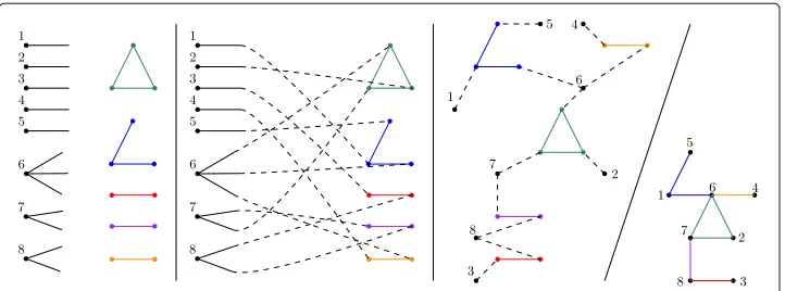
We also assume the number of community memberships of each individual is pre-scribed, and give the individual as manymembership tokens. Intuitively speaking, each community membership represents an identity that the person has, possibly including both offline identities such as a job or family role, and online identities such as an email address or a social media account. We assume that the number of community member-ships of each individual is at least one, otherwise we could remove that individual from the model. Overlaps are induced by individuals who are part of more than one commu-nity. Necessarily, the total number of tokens given to all individuals has to equal the total number of community roles available, that is, the total size of all given community graphs. The upcoming construction can be followed step by step in Fig.1. The graph is random-ized by matching the community roles with the membership tokensuniformly at random, in a one-to-one fashion. This means that each possible outcome has equal probability to be chosen, and this probability is one over the total number of possibilities. Such a match-ing can be generated sequentially: in each step, we pick an arbitrary community role, and match it with a membership token chosen uniformly at random. We then remove both objects from the available pool, and repeat the procedure until the available pool becomes empty.
Fig. 1A small example for constructing the RIGC model. From left to right, we see each step of the construction. Leftmost, we represent the list of community graphs in different colors, and the individuals by the numbered vertices; the number of stubs drawn for each individual corresponds to the number of membership tokens. The second subfigure represents the matching, with the imaginary edges drawn dashed. An imaginary edge between an individual and a vertex in a community means that one of the tokens of that individual was matched with that community role. The third subfigure is simply a redrawing of the second for the sake of clarity. Rightmost, we see the resulting RIGC, after the imaginary edges have been contracted
Visually, we can represent the matching by imaginary edges (see the second picture in Fig.1): each imaginary edge represents a membership token and a community role that are matched, and connects a vertex representing an individual to a vertex in a commu-nity graph. That is, the commucommu-nity roles taken by an individual will be connected to the individual by imaginary edges. An individual has as many imaginary edges as their pre-scribed number of tokens, and since each community role is matched with exactly one token, each is incident to exactly one imaginary edge. We note that this is not yet the ran-dom network that we are looking for, but an important intermediate step. It reflects that the only source of randomness is the matching, represented by the imaginary edges, and is a great tool throughout the analysis.
Finally, we obtain the random network by identifying each individual with the set of community roles that this individual takes. As these community roles, i.e., vertices in communities, are connected to the vertex representing the individual by imaginary edges, we can achieve this by contracting all imaginary edges (see the last picture in Fig.1).
Note that in a random matching, it might occur that we match two or more tokens of the same individual to community roles within the same community. However, this is quite unlikely. As we increase the network size, the probability for a typical individual to take several roles within any community vanishes. Also note that this may also happen in the real world, as some people may have separate work and private accounts for the same ser-vice. It may also happen that two individuals are present in several communities together, and are connected by two or more edges in the RIGC, which potentially makes the graph amultigraph. Again, we can argue that this is not unrealistic, and can be interpreted as a stronger interaction between those two individuals. Additionally, this phenomenon also becomes rare as the network size grows, allowing us tostudy the network ‘as it is’, without deleting duplicate edges and self-loops. Since the difference before and after deleting dupli-cate edges becomes negligible in the large-network limit, our asymptotic results apply to both variants of the model.
that in turn serve as crude approximations for finite, but large, network sizes. (The convergence takes place in abstract graph and distribution spaces, thus the validation of these approximations is up to future empirical research.) To allow us to compare net-works of different sizes, we assume some ‘consistency’ of the parameters, (the list of communities and the list of individuals with their number of community memberships):
Assumption 1(The parameters)We assume that in the large-network limit, i.e., as the number of individuals N→ ∞,
a) the number of communities equalsM=γN+ε(N)for some constantγ, and
ε(N)is an error term such thatε(N)/N→0;
b) for every positive integer k, the proportion of individuals with k membership tokens converges to somepk=P(T =k)≥0, where T is a random variable with finite meanE[T]<∞. Intuitively, T represents the asymptotic distribution of the number of membership tokens, arising as the limit of the empirical distributions; c) for every finite connected graph H, the relative frequency of H in the list of
communities converges to someμH ≥0, such that the collection(μH)over finite connected graphs H is a probability mass function. Thus, the proportion of communities with size k, i.e., k members, converges to someqk =P(S=k)≥0, where S is a random variable with finite meanE[S]<∞. Intuitively, S describes the asymptotic distribution of community sizes.
Note that there necessarily is a relation betweenγ,E[T] andE[S]. The reason is that the total number of membership tokens must be equal to the total size of the communities:
N(E[T]+ε1)=M·(E[S]+ε2), where the error termsε1→0 andε2→0 appear because
the empirical averages may be slightly different from their respective limits. Consequently, γ =E[T]/E[S].
A good incentive for working with pre-assigned numbers of community membership tokens for each individual is that this method allows us complete control over the distribu-tion ofT. An alternative approach inspired by the random intersection graph literature (in particular, the “active and passive” model) (Bloznelis2010; 2013; Godehardt and Jaworski
2003; Rybarczyk2011) assigns each community role to a uniformly chosen individual. While this approach makes generating the model easier, it has the disadvantage thatT
always follows a Poisson distribution, which is light-tailed. This means that the number of community memberships per individual has very small variability, which may be an undesirable property. Certain applications may call for heavy-tailed or power-law distri-butions (more on power laws later), wherehubsappear: individuals that are part of a large number of communities (up toNα, for some 1/2 < α < 1). The existence of such hubs is often crucial to the connectivity structure of the network or in making it a small world, or even an ultra-small world (see (Newman (2003b), Section 3.1) for an introduction to small and ultra-small worlds and further references). It is thus advantageous to use mem-bership tokens, as this method allows for greater generality, including both light-tailed and heavy-tailed distributions forT.
Results
basic properties such as the degree distribution and local clustering, and model-specific properties about the overlapping structure of communities. We then move to global properties, that is, structural properties of the network. In particular, we study its con-nected components, and how resilient the largest component is under randomized attack to the network.
Degrees and clustering
The upcoming sections are based on (van der Hofstad et al. 2018). Degrees, i.e., the number of connections an individual has, contain crucial information about the local structure of a network, and are easy to measure in real-world networks. For several ran-dom graph models, it has been proven that the degree distribution can make a difference between a small-world graph, where distances scale as logN in a graph of sizeN, and an ultra-small-world graph, where distances grow even slower than logN, often scaling as log logN (see (van der Hofstad2017), Section 1.4.3) for a rigorous definition); scale-free networks (defined later) are often ultra small (Bollobás and Riordan2003b; Cohen and Havlin2003). While there is no direct relation between degrees and distances, when these predictions fail, that indicates the presence of further structure in the network. Thus the degree distribution often serves as the first benchmark when tuning a model to fit a network.
Thus, the first property of the RIGC model that we study is the empirical degree distri-bution, which is random itself. There are two ways to represent this empirical distribution. The conventional representation is the sequence of proportions(nk/N), whereNdenotes
the total number of individuals, andnk denotes the random number of individuals with degreek, for all positive integersk. However, in this case working with a random sequence is not convenient. Alternatively, we can represent this empirical distribution with a sin-gle random variable. Choose a vertexV uniformly at random, and denote its degree by
DV. Then, given a realization of the graph, the probability forDV to equalkis the
prob-ability of picking a vertex with degreek, which is exactlynk/N. Thus understanding the
distribution ofDV is the same as understanding the random sequence(nk/N).
Note that in a random graph, there are two sources of randomness inDV: the choice
of the uniform individual, and the choice of the graph itself, and these are independent. In fact, these two sources of randomness help us describe the asymptotic distribution ofDV. Choosing an individual randomly means that it has a random number of
mem-bership tokens. For each token, a random community role is assigned, which adds a certain number of connections toV from that community. To formalize this, we intro-duce the random variable , such that P( = c) is the limit of the proportion of community roles that have cneighbors within their community graph. Recall the ran-dom variable T that describes the limiting distribution of the number of membership tokens.
Theorem 1(Limiting degree distribution)Leti,i ≥1be random variables indepen-dent of each other and of T, with the same distribution asdefined above. Then, for every k≥1, in the large-network limit N→ ∞,
P(DV =k)→P
T
i=1
i=k
We define the random variable D0 with the limiting distribution P(D0 = k) :=
PT
i=1i = k
. The proof of Theorem1relies on a more in-depth description of the neighborhood of a uniformly chosen individual that we intuitively discuss in the next section.
We discuss when the RIGC showcases a special type of degree distribution that has been observed (Newman2005) in real-world networks:power laws. We say thatD0follows a
power law with exponentδ > 1, ifP(D0 > x)scales asx1−δ, that is,cx1−δ < P(D0 >
x) < Cx1−δfor some constants 0 < c < Candxlarge enough. Power laws are heavy-tailed distributions, meaning that higher moments are infinite. The precise threshold is δ −1 (which may be a fractional moment): for s ≥ δ −1,EDs0 = ∞, but for any
s < δ−1,EDs0 < ∞. That is, the smallerδ is, the “heavier” the tail is, and the fewer moments exist. If for a random variable, the tailP(D0>x)decays faster than any power
ofx, we call the distribution light-tailed. In this case, all moments are finite, and we define the “power-law exponent” of such a distribution as infinity.
If the empirical degree distribution of a network of sizeN follows a power law with exponentδ, the maximal degree scales asN1/(δ−1). For the infinite-variance caseδ <3, including thescale-freecase 2< δ <3 when the mean is finite but the variance is infi-nite, this means that the largest degree is much larger thanN1/2. Such highly-connected vertices, called hubs, heavily influence the structure of the network, making the study of power-law and particularly scale-free degrees important. We identify a sufficient condi-tion for the RIGC to have power-law degrees. RecallT, the asymptotic distribution of the number of membership tokens, and, the asymptotic distribution of within-community neighbors.
Corollary 1(Power laws)If T or (or both) follow a power-law distribution, then the asymptotic degree distribution D0also follows a power law, and its exponent is the smaller
of the two exponents; intuitively speaking, the “heavier tail wins”.
When the asymptotic average degreeE[D0] is finite, the number of edges in the graph
scales asE[D0]N/2, that is, the RIGC is sparse. This happens exactly whenE[] is finite.
Next we study clustering, also known as transitivity, in the RIGC model. It has been observed (see e.g. Watts and Strogatz (1998)) that real-world networks often contain significantly more triangles than traditional random graphs with the same degree dis-tribution. In social networks, this can be explained by the fact that people who share a common friend are more likely to meet each other, through this common friend, than other people in the network. Thelocal clustering coefficientaims to capture this. For a ver-texvwith degreeDv≥2, its local clustering coefficient Cl(v)is the proportion of pairs of
neighbors ofvthat are also directly connected. This is the same as the number of triangles thatvis part of, divided byDv
2
, the total number of pairs of neighbors (if the vertex has less than two neighbors, we set Cl(v)=0). We describe the network by the average local clustering coefficient, which is the average of local clustering coefficients of each vertex.
We continue to describe the distribution of Cl(V). Again, we recognize that due to the uniform choice ofV, it has a random number of membership tokens. Due to the random matching, we match these tokens to a set of community roles chosen uniformly at random, and each community role is part of a certain number of triangles within its community. We find and show that the number of otherwise arising triangles is negligible, due to the structure of neighborhoods explained in the next section.
To formalize the result, we introduce the random variable, such thatP(=d)is the limit of the proportion of community roles that are part ofdtriangles within their own community. Note that a community role withcwithin-community neighbors is part of at most2ctriangles. Thus, with the random variablethat describes the limiting distri-bution of within-community connections,(,)form a random vector withdependent
coordinates. Recall that the random variableT describes the asymptotic distribution of the number of membership tokens.
Theorem 2(Asymptotic local clustering)Let(i,i), i ≥ 1be independent copies of the dependent random vector(,), also independent of T. For any x∈[ 0, 1], in the large-network limit N → ∞,
P(Cl(V)≤x)→P ⎛
⎝Ti=1i
T
i=1i
2
≤x
⎞
⎠=PTi=1i D0
2
≤x
=:P(Cl(0)≤x),
where we introduce the random variableCl(0)to describe the limiting distribution. The average local clustering also converges: in the large-network limit N→ ∞,
E[ Cl(V)]→E[ Cl(0)] .
For many real-life networks, the average local clustering coefficient is positive (Watts and Strogatz 1998). It is thus a desirable property for network models to have posi-tive asymptotic clustering, i.e., a posiposi-tive limit of average clustering as the network size
N → ∞. The simplest random graph models, the Erd˝os-Rényi random graph (Erd˝os and Rényi1959; Gilbert1959) and the configuration model (Bollobás1980; Molloy and Reed1995) have vanishing clustering, i.e., the average clustering goes to 0 as the network size grows. On the other hand, classical random intersections graphs and the hierarchical configuration model (with adequate parameters) produce positive asymptotic clustering. This raises interest in where the RIGC falls on this scale.
Corollary 2(Condition for positive asymptotic clustering)The RIGC produces positive asymptotic clustering exactly when there is a positive asymptotic proportion of community graphs that contain one or more triangles.
Neighborhoods and overlapping structure
In this section, we provide a more in-depth description of neighborhoods in the graph. As demonstrated by our results on degrees and (local) clustering, this is useful in deriving various properties of the graph. However, such neighborhoods are also of independent interest, to gain insight into the structure of the graph, or to measure similarity of graphs. The asymptotics of the local neighborhood structure can be conveniently described using
local weak convergence(Benjamini and Schramm 2001). We provide a brief, intuitive description here; for details and rigor of applying this notion to the RIGC, the reader is referred to (van der Hofstad et al. (2018), Sections 2.2, 4.1).
Our aim is to describe the asymptotic behavior of the neighborhood of a typical vertex in the large-network limit, and we do so by considering finite neighborhoods (see Fig.2
for a small example) of an individual chosen uniformly at random. To understand such neighborhoods, we now recall how we construct the random graph, and in particular, a neighborhood. The list of individuals, each with a given number of membership tokens, and the list of community graphs are given. Randomness solely comes from matching the membership tokens with community roles uniformly at random. We can match these two types of objects sequentially, and in each step, we can arbitrarily pick an unmatched object of either type, as long as its match is chosen uniformly at random from the unmatched objects of the other type.
As we are in a random graph, we canexplore the neighborhood of an individual by
buildingit, according to the construction rules of the random graph. Given an individ-ual whose neighborhood we want to explore, we distinguish it as theroot, and we start by matching each of its membership tokens (in some arbitrary order) to community roles chosen uniformly at random. To focus on the larger-scale structure, we enclose each community by asupervertex, and preserve the community graph itself as adecorationof the supervertex. Further, we give the supervertex as many distinguishedcommunity role
tokensas the size of the enclosed community. In ourstructural graph, the supervertices representing communities that the root is part of become direct neighbors of the root and formlayer 1.
Next, we explore all further individuals in the communities of layer 1; we match each community role (in some arbitrary order) to a uniformly chosen membership token. These membership tokens belong to some individuals, and these individuals formlayer 2. Matching the remaining membership tokens of the layer 2 individuals, we reach another set of communities, that become the supervertices of layer 3, and so on. Every odd layer contains supervertices that represent communities first entered through individuals in the previous layer; every even layer contains individuals first found in communities in the previous layer. In the structural graph that we build this way, edges represent a match between a membership token and a community role token, thus they correspond to imaginary edges from the construction.
This structural graph islocally tree-like: up to a finite number of layers, it is less and less likely to see a cycle as the network size grows. (Note that this holds on the structural level only; cycles contained in the community graphs are preserved in the network.) The reason behind this phenomenon is that we match membership tokens and community rolesuniformlyat random, thus the probability of choosing from a set is proportional to its size. The community sizes and the number of tokens are small relative to the network size, thus the set of tokens within a finite number of layers becomes negligible compared to the total pool that increases with the network size. Consequently, re-connecting to an already seen individual or supervertex and thus creating a cycle becomes unlikely.
This observation suggests that in the limit, the neighborhood of a typical vertex becomes a decorated randomtree, where the tree describes the membership relations of individuals and communities, and the decorations describe the communities. In the fol-lowing, we explain the law of this decorated tree, which is in fact a branching process (see (Athreya and Ney2004) for an introduction to branching processes). For our purposes here, it is sufficient to think of it as a random tree that is constructed layer by layer from a root, and each vertex has anindependentrandom number ofoffspringin the next layer. The root corresponds to a individual chosen uniformly at random, thus the number of its offspring is drawn from the asymptotic distribution of tokensT. However, the offspring distribution of further layers is affected by the fact that we match themembership tokens
andcommunity rolesuniformly at random. Thus, a community with sizekisktimes more likely to be chosen than a community of size 1. This effect is calledsize-biasing. Also note that a community of sizekproducesk−1 individuals as offspring, since one of its members is in the previous layer.
Thus, for the asymptotic distribution of community sizesS, we introduce its size-biased versionSwith mass functionPS=k−1= kP(S= k)/E[S]. Similarly for the asymp-totic number of tokensT, we defineT with mass function PT =k−1 = kP(T = k)/E[T]. This describes the random tree, and we decorate it as follows. Given that a com-munity has size k (offspringk−1), its community graph is chosen with probabilities proportional to the limiting frequenciesμH(see Assumption1), for connected graphsH
onkvertices. That is, the probability of choosing a particular graphHonkvertices equals μH/P(S=k).
step as theprojection. First, we ‘blow up’ the supervertices into the communities they rep-resent. This graph corresponds to the intermediate step in the construction, where the matching is represented by imaginary edges; the role of the imaginary edges is now taken by the edges of the random tree. Thus, the second step is to contract the original edges of the random tree, and we obtain the limit of the network, from the perspective of a typical individual.
Next, we discuss how the locally tree-like nature of the structural graph impacts the overlapping structure of communities. We say that two communities overlap, or are neighbors, when they share one or more individuals; the size of the overlap is the number of individuals shared.
Theorem 3(Single-overlap property)The number of overlapping pairs of communities scales linearly with the network size N, that is, a community chosen uniformly at random overlaps with constantly many others.
The “typical” overlap between overlapping communities is a single individual.
More precisely, with probability tending to 1 in the large-network limitN→ ∞:
i) an individual chosen uniformly at random is not part of an overlap larger than 1, i.e., it is not part of several communities together with any other individual; ii) a community chosen uniformly at random does not overlap in more than one
individual with any other community.
This means that overlaps of size 2 or higher may still occur, but their number is sublinear in the network sizeN, and consequently also sublinear in the number of communitiesM, as well as the total number of overlaps.
The single-overlap property allows for community detection with good accuracy in a special case, inspired by clique-percolation (Derényi et al.2005). We say that a graph is triangle-connected, if we can connect any two vertices by a chain of triangles such that each consecutive pair shares an edge. (This is a special case ofk-clique-connected graphs fork = 3.) Assume that all community graphs are triangle-connected; this is a slightly stronger condition than assuming that the graph is connected and each vertex is part of at least one triangle. In fact, such a graph can be constructed by adding triangles one by one so that each new triangle shares an edge with one of the old ones. This construction can serve as a greedy algorithm to find such a community. If an arbitrary community only shares overlaps of size 1 with any neighboring community, it cannot share an edge with them, and thus our greedy algorithm will detect the boundaries of this community exactly. Considering the RIGC with triangle-connected communities, with probability tending to 1, the graph realization is “nice” and only a sublinear proportion of communities share an overlap of 2 or larger. Thus only a sublinear proportion of communities are misdetected.
Connected components
First, we observe that the internal structure of the communities does not have any influ-ence on the global connectivity structure. The reason behind is that we have assumed each community to be connected in itself, thus it provides a path between any two com-munity members, even if they are not directly connected. Indeed, our results below only depend on the community sizes and the distribution of membership tokens of individuals.
We find that component sizes are closely related to the decorated branching process, introduced in the section above (p. 10). Recall that this branching process captures the local structure of the graph, treating communities as supervertices, and the network is obtained by a projection: ‘blowing up’ the supervertices into the communities they rep-resent, and then contracting the tree edges. For simplicity, we will utilize and refer to the random tree, keeping in mind this distinction. Intuitively, the component of an individ-ual is its neighborhood, for which a corresponding decorated branching process provides an approximate description. Roughly speaking, if the tree is small, then the component is small; if the tree grows unbounded, i.e., is infinite, then the component is large com-pared to the network size. (We omit the technicalities why this reasoning stands even when the component size isnotnegligible compared to the network size; however, this is not surprising, as similar phenomena appear in commonly used random graph mod-els such as the Erd˝os-Rényi random graph (Alon and Spencer (2008), Section 10.5) or the configuration model (Molloy and Reed1995)).
Thus, we first investigate the behavior of this random tree, which is largely defined by the offspring distributionsTandS, and we discuss the effect of the root having offspring
T later. It is well known that a branching process undergoes aphase transition, i.e., it shows largely different behavior based on the choice of a parameter. The behavior we are interested in is whether the tree has a positive probability of growing infinitely. The phase transition happens atE[T]E[S]=1.
The reason for this is thatE[T]E[S] is the expected growth ratio between two consec-utive layers that contain individuals. Thus, ifE[T]E[S]> 1, the expected size of layers containing individuals grows exponentially; in this case, the tree is infinite with some positive probability ξ, and we say that the branching process is supercritical. On the contrary, ifE[T]E[S]< 1, the expected size of layers containing individuals decreases exponentially, and the random tree is almost surely finite; we call the branching process subcritical.
The phase transition of the branching process translates to the component sizes in the RIGC model as follows. In the subcritical case, when the random tree is almost surely finite, the graph consists of small components; most are of constant size, and all are sub-linear in the network size. In the supercritical case, the random tree has probabilityξ to be infinite, and aξ proportion of individuals has such a corresponding branching pro-cess. Clearly, individuals within a finite graph cannot have an infinite component, instead all such vertices join together and form agiant component: a unique linear-sized com-ponent. The remaining components are all ‘small’, in the same sense as in the subcritical case.
We summarize our findings in the theorem below:
i) In the subcritical (and critical) caseE[S]E[T]≤1, all components of the RIGC are sublinear in the network size N.
ii) In the supercritical caseE[S]E[T]>1, the largest component contains a
proportionξ of all individuals. This component is unique: all other components are sublinear in the network size N.
The statements above hold with probability tending to 1 as the network size N → ∞.
We note that there is a lower order probabilistic error in the size of the giant component; in particular,ξ = 1 does not necessarily mean that the whole graph is connected, but the individuals outside the giant only make up a sublinear proportion. (Identifying the conditions under which the RIGC is connected is outside the scope of this paper.)
In fact, we can identifyξ, the probability that the branching process produces an infinite tree, in terms ofprobability generating functions(PGF). We define the PGF of a non-negative integer valued random variableXas PGFX(z):=k∞=0zkP(X=k). Recall thatT
denotes the asymptotic distribution of tokens, and the root of the branching process has offspringT. Also recall that, due to matching membership tokens and community roles uniformly, the rest of the offspring are size-biased, and we introduced the distribution PT =k−1 = kP(T = k)/E[T]. Similarly, for the asymptotic community sizeS, we introducedS. Denote byηthe smallest non-negative solution to the fixed-point equation
z=PGFS
PGFT(z)
, thenξis given byξ=1−PGFT(η).
In the following, we obtain further properties of the giant component by applying the previous reasoning: that an individual is part of the giant component exactly when the corresponding branching process produces an infinite tree. (This is true, except for a negligible sublinear proportion of individuals.) Keep in mind that the limit of the neigh-borhood is obtained from the decorated branching process by a projection: ‘blowing up’ the supervertices into the communities they represent and then contracting the edges of the branching process.
Corollary 3(Degrees and edges in the giant) Consider the empirical degree distribu-tion of the giant component, or equivalently, the degree of an individual chosen uniformly at random within the giant component. This converges to the degree of the root in the projection of the decorated branching process that is conditioned on being infinite.
If the mean of this limiting degree distribution ism<∞, then the number of edges in the giant component scales asmξN/2. If this mean is infinite, the number of edges in the giant component is superlinear in the network size.
We intuitively explain why conditioning the random tree on being infinite generally
the giant component to be larger than the average degree in the entire network. However, as the communities are arbitrary, the opposite may occur.)
Information spread and attack vulnerability
In the previous section, we have focused on connected components, as each component is a set of individuals that may interact. On the other hand, certain interactions, such as the spread of a virus, be it a biological or computer virus, may very well be non-deterministic. As a simplistic model for a random spread, we considerpercolation: for each edge, we flip ap-coin, independently of each other, to randomize whether that edge is able to transmit. With probabilityq =1−p, we consider an edge unable to transmit and remove it from the graph; we call the remaining subgraph thepercolatedgraph. We emphasize that when we talk aboutp-percolation,p ∈[0, 1] is the probability that an edge is considered to be able to transmit and is kept (retained); in particular,p= 1 yields the original graph and
p=0 yields the empty graph.
Consider a simple epidemic spread, called SI-epidemic, named after the two possible states of individuals: susceptible or infected. We start the spread by setting a single indi-vidual as infected. Time progresses in discrete steps and the dynamics afterwards are as follows: all the individuals that became infected in the previous step attempt to transmit the infection through all incident edges, all of which succeed independently with proba-bilityp. If a yet susceptible neighbor is reached, then we set it as infected. Each individual only attempts to spread the infection once. When no new individual becomes infected, the process stops.
For the SI-infection model, even such a simple static model as percolation is able to capture the final infected cluster: all vertices that are connected to the source of infec-tion in the percolated graph will eventually be infected. This, again, raises interest in the component sizes of the percolated graph: if there is a large component after percolation, there is a possibility for a large viral outbreak, in case the source is chosen from this large component.
There is always a trade-off in modeling: realistic models tend to be more complex, while simple models are easy to analyze. In the case of percolation, its simplicity has yet another advantage: it leaves room for different interpretations. We can also consider the inde-pendent removal of edges as a randomized attack on the network, in which case we are interested in how well the network can withstand such attacks. Once again, we arrive at the same question from a different perspective: what remains of the giant component, if we randomly remove a proportion 1−pof the edges?
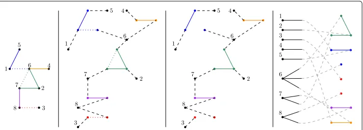
By definition, percolation on the RIGC model means that we first generate the random graph, and then, conditionally on the graph realization, randomly retain or remove each edge. However, recall that we construct the graph by adding imaginary edges randomly between individuals and community roles, and then contracting these imaginary edges. Thus, the edges of the resulting graph correspond one-to-one to the collection of all edges from all community graphs. This means that the percolation in fact doesnotdepend on the graph realization. Moreover, we may even change the order: percolate the edges within the community graphs first, and then generate the RIGC, see Fig.3.
the condition that each community must be connected, we separate each connected com-ponent as its own community. This creates a new, random list of communities, that typically contains more, but smaller communities than the original unpercolated list, and we refer to it as thepercolated community list. We can now formalize our observations as follows:
Proposition 1(Percolated RIGC)Percolation on the RIGC model is another RIGC, with the percolated community list and the original list of individuals and original number of membership tokens. In particular, percolation on the classical random intersection graph, i.e., when each community is a complete graph, is also an RIGC.
With Proposition1and Theorem4in hand, we have the recipe for identifying the super-critical and subsuper-critical cases ofpercolationon the RIGC. We assume that the original RIGC is supercritical, so that a giant component exists, and study for which choices ofp
the percolated graph is supercritical.
We note that the percolated community list sensitively depends on the original struc-ture of the communities. This is in contrast with the observation that the global con-nectivity structure did not depend on the internal structure of communities,as long as they are connected. At the same time, this comparison also serves as an explanation why community structure now matters: it determines how the community falls apart under percolation, in particular, how many and how large components are produced.
Let us introduce the limiting community size distribution of thepercolatedcommunity list and denote it byS(p). Recall the limiting distributionTof the number of membership tokens, and its size-biased versionT, given byPT =k−1= kP(T = k)/E[T]. Simi-larly, defineS(p)byP S(p)=k−1=kP(S(p)=k)/E[S(p)]. It follows from Theorem4
that the condition for supercriticality isET E S(p) >1. Keep in mind that we consider this as an implicit condition onp.
The closerpis to 1, the more edges we keep, and the larger the percolated community sizes are, thusE S(p) is increasing inp. Consequently, we can find a threshold value (crit-ical percolation parameter)pcand write the supercriticality condition explicitly asp>pc.
This thresholdpcis the smallestp(more precisely, the infimum ofpvalues) such that
ET E S(p) >1. Under some mild regularity conditions, e.g.ET2 <∞andES2 < ∞is sufficient,pcis simply the solution to the implicit equationET E[S(pc)]=1. (We
give a counterexample later.)
Corollary 4 (Percolation phase transition) Percolation on the supercritical RIGC exhibits a phase transition as we vary the percolation parameter p. With0 ≤ pc < 1
defined above,
i) in the subcritical casep<pc, the largest component of the percolated graph is sublinear in the network size N;
ii) in the supercritical casep>pc, there exists a unique, linear-sized component that contains a proportion0< ξ(p)≤ξof the individuals.
The statements above hold with probability tending to 1 as N→ ∞.
In the following, we provide a discussion on Corollary4and some special cases, with an emphasis on attack vulnerability.
The casep= pcwas excluded, as it is open in some particular instances. Under some regularity conditions, i.e.,ES2 <∞andET2 <∞, we haveET E[S(pc)]=1, thus
the graph shows so-called critical behavior. It is alike with the subcritical case in the sense that the largest component is sublinear, but shows more subtle differences. However, an in-depth discussion of critical behavior is beyond the scope of this paper.
The fact thatpc < 1 always holds means that the network does not exhibitinstant failure. This means that the network may lose a linear proportion of edges, and as long as this fraction is small enough, a smaller, but still linear-sized giant component is retained. The intuitive reason for this is that whenpis close enough to 1, small communities do not suffer too much damage, and that is sufficient to hold a good proportion of the network together.
On the other end of the spectrum, it is possible thatpc= 0, depending on the choice
of parameters, which we discuss later in more detail. If pc = 0, then for arbitrarily small ε, if at least an ε proportion of edges is kept, a small, but linear-sized compo-nent persists. This phenomenon is calledrobustness, and a robust network can withstand randomized attacks very well. It has been observed that manyscale-freenetworks and models are robust (Bollobás and Riordan2003a; Cohen et al.2000; Solé and Montoya
2001). Scale-free, as before, refers to a network with a power-law degree distribution with exponent τ ∈ (2, 3); that is, degrees with finite mean but infinite variance. In such a network, the hubs, i.e., the highest-degree vertices with degree larger thanN1/2, hold the network together against random attacks. In the case of the RIGC, the hubs may be both large communities and individuals with a large number of membership tokens.
the traditional finite variance condition, we consider whetherET2 andES2 are finite. However, there is another reason for considering these quantities: their relation toET
andES respectively, explained below.
As discussed after Proposition1, percolation with edge retention probabilitypis super-critical when ET E S(p) > 1. As discussed before, E S(p) is a non-decreasing function ofp; sincep=0 yields the empty graph andp=1 yields the original graph, the values ofET E S(p) range from 0 toET ES . It is thus crucial whetherET ES
is finite. Recall that we have defined the size-biased versionTasP(T =k−1)=kP(T= k)/E[T]. Consequently,ET =E[T(T−1)]/E[T] is finite exactly whenET2 is finite, and similarly,ES is finite exactly whenES2 is finite.
The simplest, ‘regular’ case is whenET ES is finite, i.e., bothET andES are finite. This corresponds to the classical non-scale-free case and the graph isnon-robust.
IfET is infinite, irrespective of whetherES is finite, the graph isrobust. The rea-son is that some individuals are hubs and are part of a polynomially large number of communities, and have at least one incident edge in each. Thus, as long as an arbitrar-ily small, but positive proportion of edges is retained, these individuals remain hubs and hold a considerable proportion of the network connected. Indeed, for any small but pos-itivep,E S(p) is positive and thusET E S(p) is infinite. Also note that in this case the equationE S(p) ET = 1 does not have a solution, as atp=0, we have an empty graph and this quantity becomes 0.
The most interesting and most complex case is whenES is infinite, butET is finite. This means that the hubs are the communities, and the communities only, thus depending on the exact limiting distribution of community graphs(μH), the RIGCmay or may not be robust. Intuitively, when the large community graphs are dense enough, e.g. when all communities are complete graphs, the total edge count of the RIGC becomes superlinear, and consequently the graph is robust. On the other hand, when large community graphs are sparse, e.g. have bounded within-community degree independent of the community size, these communities fracture into many small pieces under percolation, and the graph is not robust. It remains an intriguing open question what happens in between, as the dependence on(μH)is hard to quantify.
Conclusion
The model we introduce, the random intersection graph with communities, fills a gap in the literature in modeling networks with community structure, where communities are allowed to overlap and at the same time have their own internal structure. Built in a random fashion with arbitrary small graphs as building blocks, it is well-fitted to model networks with well-defined local structure but a more fluid global structure. Consider a social network where the internal structure of a community is determined by its purpose, e.g. whether it is a family or a workplace, while the variability in the combination of roles people take on is so vast that it can be considered random over the population. This large-scale randomness allows us to carry out exact asymptotic calculations.
for modeling real-world networks. In the global structure, such as connectivity, generic macroscopic effects emerge despite the particular microscopic structures. However, the existence these microscopic structures, in particular, the fragility of communities, once again plays a crucial role in spreading processes or randomized attacks on the network.
Abbreviations
HCM: hierarchical configuration model; RIG: random intersection graph; RIGC: random intersection graph with communities
Acknowledgements
The authors thank the anonymous reviewers for their helpful insights and suggestions that helped to improve the presentation of this paper.
Authors’ contributions
VV performed a major part of the mathematical analysis of the proposed model, as well as of the writing of the paper. JK contributed to the mathematical analysis of the proposed model as well as revised the manuscript critically for important intellectual content. RvdH has contributed to the design of the model and its mathematical analysis. All authors have read and approved the final manuscript.
Funding
This work is supported by the Netherlands Organisation for Scientific Research (NWO) through VICI grant 639.033.806 (RvdH), VENI grant 639.031.447 (JK), the Gravitation NETWORKSgrant 024.002.003 (RvdH), and TOP grant 613.001.451 (VV). The Gravitation NETWORKSgrant and TOP grant played a major role in conceptualizing the study of networks with community structures, in particular spreading processes on such networks. None of the funding influenced the outcome of the mathematical analysis.
Availability of data and materials
Not applicable.
Competing interests
The authors declare that they have no competing interests.
Received: 12 November 2018 Accepted: 28 May 2019
References
Alon N, Spencer JH (2008) The Probabilistic Method. 3rd ed. Wiley-Interscience Series in Discrete Mathematics and Optimization. Wiley, Hoboken. With an appendix on the life and work of Paul Erd ˝os.https://doi.org/10.1002/ 9780470277331
Athreya KB, Ney PE (2004) Branching Processes. Dover Publications, Inc., Mineola. Reprint of the 1972 original [Springer, New York; MR0373040]
Ball F, Sirl D, Trapman P (2009) Threshold behaviour and final outcome of an epidemic on a random network with household structure. Adv Appl Probab 41(3):765–796.https://doi.org/10.1239/aap/1253281063
Ball F, Sirl D, Trapman P (2010) Analysis of a stochastic SIR epidemic on a random network incorporating household structure. Math Biosci 224(2):53–73.https://doi.org/10.1016/j.mbs.2009.12.003
Benjamini I, Schramm O (2001) Recurrence of distributional limits of finite planar graphs. Electron J Probab 6:23–13. https://doi.org/10.1214/EJP.v6-96
Bloznelis M (2010) Component evolution in general random intersection graphs. SIAM J Discrete Math 24(2):639–654. https://doi.org/10.1137/080713756
Bloznelis M (2013) Degree and clustering coefficient in sparse random intersection graphs. Ann Appl Probab 23(3):1254–1289.https://doi.org/10.1214/12-AAP874
Bloznelis M, Godehardt E, Jaworski J, Kurauskas V, Rybarczyk K (2015) Recent progress in complex network analysis: properties of random intersection graphs. In: Data Science, Learning by Latent Structures, and Knowledge Discovery. Stud. Classification Data Anal. Knowledge Organ. Springer, Heidelberg. pp 79–88
Bollobás B (1980) A probabilistic proof of an asymptotic formula for the number of labelled regular graphs. Eur J Comb 1(4):311–316
Bollobás B (2001) Random Graphs, 2nd edn. Cambridge Studies in Advanced Mathematics, vol. 73. Cambridge University Press, Cambridge.https://doi.org/10.1017/CBO9780511814068
Bollobás B, Riordan O (2003a) Robustness and vulnerability of scale-free random graphs. Internet Math 1(1):1–35 Bollobás B, Riordan OM (2003b) Mathematical results on scale-free random graphs. In: Handbook of Graphs and
Networks. Wiley-VCH, Weinheim. pp 1–34
Cohen R, Havlin S (2003) Scale-free networks are ultrasmall. Phys Rev Lett 90:058701.https://doi.org/10.1103/ PhysRevLett.90.058701
Cohen R, Erez K, Ben-Avraham D, Havlin S (2000) Resilience of the internet to random breakdowns. Phys Rev Lett 85:4626–4628.https://doi.org/10.1103/PhysRevLett.85.4626
Deijfen M, Kets W (2009) Random intersection graphs with tunable degree distribution and clustering. Probab Engrg Inform Sci 23(4):661–674.https://doi.org/10.1017/S0269964809990064
Erd ˝os P, Rényi A (1959) On random graphs. I. Publ Math Debrecen 6:290–297 Gilbert EN (1959) Random graphs. Ann Math Stat 30(4):1141–1144
Godehardt E, Jaworski J (2003) Two models of random intersection graphs for classification(Schwaiger M, Opitz O, eds.). Springer, Berlin.https://doi.org/10.1007/978-3-642-55721-7_8
Guillaume J-L, Latapy M (2004) Bipartite structure of all complex networks. Inform Process Lett 90(5):215–221.https://doi. org/10.1016/j.ipl.2004.03.007
Guillaume J-L, Latapy M (2006) Bipartite graphs as models of complex networks. Phys A Stat Mech Appl 371(2):795–813 van der Hofstad R, Komjáthy J, Vadon V (2018) Random intersection graphs with communities. arXiv:1809.02514 van der Hofstad R (2017) Random Graphs and Complex Networks. Vol. 1. Cambridge Series in Statistical and Probabilistic
Mathematics, vol. 43. Cambridge University Press, Cambridge.https://doi.org/10.1017/9781316779422
van der Hofstad R (2018+) Random Graphs and Complex Networks. Vol. 2. Available athttp://www.win.tue.nl/~rhofstad/ NotesRGCNII.pdf
van der Hofstad R, Komjáthy J, Vadon V (2019) Phase transition in random intersection graphs with communities. arXiv:1905.06253
van der Hofstad R, van Leeuwaarden JSH, Stegehuis C (2016) Hierarchical configuration model. Internet Math.https://doi. org/10.24166/im.01.2017
Janson S, Łuczak T, Rucinski A (2000) Random Graphs. Wiley-Interscience Series in Discrete Mathematics and Optimization. Wiley-Interscience, New York.https://doi.org/10.1002/9781118032718
Karjalainen J, Leeuwaarden JSHv, Leskelä L (2018) Parameter estimators of sparse random intersection graphs with thinned communities. In: International Workshop on Algorithms and Models for the Web-Graph. Springer, Cham. pp 44–58
Karonski M, Scheinerman ER, Singer-Cohen KB (1999) On random intersection graphs: The subgraph problem. Comb Probab Comput 8(1&2):131–159
Molloy M, Reed B (1995) A critical point for random graphs with a given degree sequence. In: Proceedings of the Sixth International Seminar on Random Graphs and Probabilistic Methods in Combinatorics and Computer Science, “Random Graphs ’93” (Pozna ´n, 1993), vol. 6. pp 161–179.https://doi.org/10.1002/rsa.3240060204
Newman MEJ (2010) Networks. Oxford University Press, Oxford.https://doi.org/10.1093/acprof:oso/9780199206650.001. 0001
Newman ME (2003a) Properties of highly clustered networks. Phys Rev E 68(2):026121 Newman ME (2003b) The structure and function of complex networks. SIAM Rev 45(2):167–256 Newman ME (2005) Power laws, Pareto distributions and Zipf’s law. Contemp Phys 46(5):323–351
Rybarczyk K (2011) Diameter, connectivity, and phase transition of the uniform random intersection graph. Discret Math 311(17):1998–2019
Singer KB (1996) Random Intersection Graphs. ProQuest LLC, Ann Arbor. Thesis (Ph.D.)–The Johns Hopkins University. http://gateway.proquest.com/openurl?url_ver=Z39.88-2004&rft_val_fmt=info:ofi/fmt:kev:mtx:dissertation&res_dat= xri:pqdiss&rft_dat=xri:pqdiss:9617602
Solé RV, Montoya M (2001) Complexity and fragility in ecological networks. Proc R Soc London Ser B Biol Sci 268(1480):2039–2045
Stegehuis C, van der Hofstad R, van Leeuwaerden JSH (2016a) Epidemic spreading on complex networks with community structures. Sci Rep 6. article number: 29748
Stegehuis C, van der Hofstad R, van Leeuwaerden JSH (2016b) Power-law relations in random networks with communities. Phys Rev E 94:012302.https://doi.org/10.1103/PhysRevE.94.012302
Vázquez A, Pastor-Satorras R, Vespignani A (2002) Large-scale topological and dynamical properties of the internet. Phys Rev E 65:066130.https://doi.org/10.1103/PhysRevE.65.066130
Watts DJ, Strogatz SH (1998) Collective dynamics of ‘small-world’ networks. Nature 393(6684):440
Ya ˘gan O (2016) Zero-one laws for connectivity in inhomogeneous random key graphs. IEEE Trans Inform Theory 62(8):4559–4574.https://doi.org/10.1109/TIT.2016.2574742
Ya ˇgan O, Makowski AM (2012) Zero-one laws for connectivity in random key graphs. IEEE Trans Inform Theory 58(5):2983–2999.https://doi.org/10.1109/TIT.2011.2181331
Publisher’s Note