DOI 10.1007/s13173-011-0050-6 S I : G R A P H C L I Q U E S
Branch and bound algorithms for the maximum clique problem
under a unified framework
Renato Carmo·Alexandre Züge
Received: 14 November 2011 / Accepted: 23 November 2011 / Published online: 24 December 2011 © The Brazilian Computer Society 2011
Abstract In this paper we review branch and bound-based algorithms proposed for the exact solution of the maximum clique problem and describe them under a unifying concep-tual framework. As a proof of concept, we acconcep-tually imple-mented eight of these algorithms as parametrized versions of one single general branch and bound algorithm.
The purpose of the present work is double folded. In the one hand, the implementation of several different algo-rithms under the same computational environment allows for a more precise assessment of their comparative perfor-mance at the experimental level. On the other hand we see the unifying conceptual framework provided by such de-scription as a valuable step toward a more fine grained anal-ysis of these algorithms.
Keywords Maximum clique·Exact solution·Branch and bound
1 Introduction
TheMaximum Cliqueproblem (MC) is the problem of find-ing a clique of maximum size on a given graph.
There are a number of proposed algorithms for the ex-act solution ofMCwhich are reported to effectively solve instances of practical interest (some of them of considerable size) in several domains [3,9,17]. Among these, branch and
R. Carmo (
)·A. ZügeDepartamento de Informática da UFPR Centro Politécnico da Universidade Federal do Paraná, Curitiba, PR, Brasil 81531-990, P.O. Box 19081
e-mail:[email protected] A. Züge
e-mail:[email protected]
bound-based schemes stand out in the literature as one of the best approaches in practice.
More often than not, these algorithms are published from an experimental standpoint, where running times for several testing benchmarks are given and commented upon, but lit-tle or no analytic results are given in support of the verified performance. On the other hand the currently available re-sults on the asymptotic behavior of algorithms forMCseem to leave a considerable gap between the worst case perfor-mance and the one actually reported by experimental results. In this paper we review eight of these algorithms and de-scribe them under a unifying conceptual framework. Besides surveying some of the best performing algorithms published to date, we aim to contribute with some perspective on the subject of branch and bound algorithms forMCfrom both, conceptual and experimental standpoints.
The unified framework introduced in the following sec-tions invites to an implementation in which each of the al-gorithms discussed becomes a particular variation of a gen-eral branch and bound algorithm forMC. We actually imple-mented each of them in this way and present experimental results on their performance under the same computational environment, something which is not available in the litera-ture to the best of our knowledge.
in Sect.3, and we present comparative experimental results from our implementation, all obtained under the same com-putational environment. In Sect.5we discuss some imple-mentation details and make our concluding remarks. In the Appendix, we include the unabridged version of the experi-mental results presented in Sect.4.
1.1 Definitions and notation
Given a setSand an integerk we denote bySkthe set of subsets ofSof sizek.
AgraphGis a pair(V (G), E(G))whereV (G)is a finite set and E(G)⊆V (G)2 . The elements ofV (G) andE(G) are calledverticesandedgesofG, respectively. Two vertices u andv are said to beneighborsinGif{u, v}is an edge in G. The neighborhood of a vertex v inG is the set of its neighbors in Gand is denoted ΓG(v). Thedegreeof a vertexvinGis the size of its neighborhood inG. Given a setS⊆V (G)the common neighborhoodofS inGis the set of vertices in G which are neighbors to all vertices in S and is denotedΓG∩(S). It will be convenient to adopt the convention thatΓG∩(∅)=V (G).
A graphGis said to becompleteifE(G)=V (G)2 . IS⊆ V (G), thesubgraph ofGinduced by a setS⊆V (G)is the graphG[S] =S,2S∩E(G)andG−Sdenotes the graph G[V (G)−S]. AcliqueinGis a set of vertices ofGthat induces a complete graph. The size of a maximum clique in Gis denotedω(G).
Given an integerk, ak-coloringofGis a surjective func-tionγ:V (G)→ {1, . . . , k}satisfyingγ (u)=γ (v)for every {u, v} ∈E(G). The value ofγ (v)is called thecolorofvand the integerkis called thenumber of colorsinγ. Acoloring ofGis ak-coloring ofGfor some integerk. We note that ω(G)≤kfor any graphGand anyk-coloring ofG.
Alist of verticesofGis a sequenceL=(v1, . . . , vn)of distinct vertices ofGwithn= |V (G)|. A coloringγ ofG isgreedywith respect to the listLif the color of each vertex vi: 1≤i≤nis the minimum not in{γ (vj): 1≤j < i}.
In the use of the notation above, we omit subscripts and superscripts whenever this can be done without ambiguity.
2 Exact solution of the maximum clique problem
TheMaximum Cliqueproblem (MC) is the problem of find-ing a clique of maximum size on a given graph. More pre-cisely, an instance toMCis a graphGand a solution to in-stanceGis a clique of maximum size inG. The problem is NP-hard [7] and cannot even be approximated in polyno-mial time up to a factor of|V (G)|1/3[1].
Several approaches have been proposed to the exact so-lution ofMC. A nice survey can be found in [3]. Concerning the actual implementation of exact solutions forMCtargeted
at general (as opposed to particular classes of) instances, branch and bound-based approaches stand out with respect to the verified performance, besides being relatively easy to implement. In a sense that will be made more precise in Sect.3, the majority of branch and bound algorithms forMC can be seen as based on the algorithm of Bron–Kerbosch [4] for enumerating all maximal cliques of a graph. We will refer to such algorithms asBK-based algorithms.
A graph onnvertices can have as much as 3n/3 differ-ent maximal cliques [11]. Therefore, any algorithm which enumerates all maximal cliques of a graph on n vertices must have worst case running time of Ω(3n/3). An algo-rithm matching this lower bound with worst case running time ofO(3n/3)was introduced in [19].
On the other hand, finding the maximum clique of a graph does not require to actually examine all of its max-imal cliques. Along the search among the maxmax-imal cliques of the graph, some non-maximal cliques can be discarded as soon as they are identified as not contained in a clique larger than another already known. That the number of discarded cliques in such a strategy can be significant is shown in [15] which introduces an algorithm forMCwith worst case run-ning time of O(2n/3). This bound was later improved to O(20.304n)[8] and further toO(20.276n)[13]. Presently the value of this bound is set toO(20.249n)[14].
Reports from the “experimental front”, however, sug-gest that worst case estimates do not tell the whole story. Indeed, several authors who implementedBK-based algo-rithms forMCreport running times which may be surpris-ing when confronted to the best known worst case estimates (besides [5,6,9,16–18] which are discussed below, see also [10,12]).
Experimental results forMCin the literature are usually obtained using two main classes of instances, namely, random graphs: sets of graphs generated according to the
Gn,p model [2], for different values of the parameters n (number of vertices) andp(edge probability).
DIMACSgraphs: a set of 66 graphs from theDIMACS Sec-ond Implementation Challenge.1
Many of these algorithms are published with the focus on the benchmarking, while little (if any at all) concern is given to the analysis of the proposed algorithm. Explaining the gap between the disheartening worst case estimates and what has actually already been achieved in practice seems to be an interesting challenge. With this long term goal in mind, in the next section we reframe theBK-based algorithms in a unifying form.
3 A general branch and bound algorithm
In this section we focus on algorithms forMCbased on the enumerating algorithm of Bron–Kerbosch [4], which we call BK-based algorithms. We start by stating Bron–Kerbosch’s algorithm in a form that highlights its main idea. The Bron– Kerbosch’s algorithm is not an algorithm for MC. Rather, it solves the related problem of enumerating all maximal cliques of a given graph. We proceed to a straightforward conversion of our statement of Bron–Kerbosch algorithm into a non-recursive algorithm forMCand thence to a gen-eral branch and bound algorithm from whichBK-based al-gorithms can be easily derived.
Let G be a graph and consider the Algorithm BK(G, Q, N ) below, where Qis a clique in Gand N ⊆ V (G)−Q.
BK(G, Q, N ) IfΓG∩(Q)= ∅
1
Return{Q}
2
IfΓG∩(Q)−N⊆ΓG(v)for somev∈N
3
Return∅
4
v←a vertex fromΓG∩(Q)−N
5
Return BK(G, Q∪ {v}, N )∪BK(G, Q, N∪ {v})
6
Algorithm BK makes explicit the enumeration scheme proposed in [4]. The idea of the algorithm is clear once we notice that ifGis a graph,Qis a non-empty clique inGand N⊆V (G)−Q, thenBK(G, Q, N )is the set of all maximal cliques ofGcontainingQwhich do not intersectN.
Algorithm BK can be converted into algorithm MAXCLIQUEbelow in a straightforward way as follows.
MAXCLIQUE(G) C← ∅
1
S ← {(∅, V (G))}
2
WhileS = ∅
3
(Q, K)←pop(S)
4
WhileK= ∅
5
v←remove(K)
6
S ←push(Q, K)
7
(Q, K)←(Q∪ {v}, K∩Γ (v))
8
If|C|<|Q|
9
C←Q
10
ReturnC
11
In Algorithm MAXCLIQUEwe have the following. 1. At any given point of the execution, the setC stores the
maximum clique inGfound up to that point of the exe-cution.
2. The setS is a stack (“last in first out”) data structure, implementing the recursion in Algorithm BK.
3. The statementv←remove(K)means that some vertex is removed from setKand left in variablev.
4. Each pair (Q, K) corresponds to the pair of sets (Q, ΓG∩(Q)−N )in Algorithm BK.
In order to convert Algorithm MAXCLIQUEinto a branch and bound algorithm for MC, we add a bounding scheme which allows us to discard a pair(Q, K)from the stackS if we detect that this pair cannot possibly lead to a clique larger thanC. We also add some pre and post-processing routines which will be discussed in the sequel.
MAXCLIQUEBB(G) (C,S)←pre-process(G)
1
WhileS = ∅
2
(Q, K)←pre-process-state(G,pop(S), C)
3
WhileK= ∅and|C|<|Q| +bound(G, Q, K)
4
v←remove(K)
5
S ←push(G, Q, K)
6
(Q, K)←pre-process-state(G, Q∪ {v},
7
K∩Γ (v), C) If|C|<|Q|
8
(C,S)←update(G, C,S, Q)
9
Returnpost-process(G, C)
10
In Algorithm MAXCLIQUEBB we have the following. 1. pre-process(G)returns the initial values ofC andS. 2. pre-process-state(G, Q, K, C) returns a state (Q, K)
whereQ−Q⊆K−K. Note that this includes the case (Q, K)=(Q, K).
3. bound(G, Q, K)returns an integerb≥ω(G[K]). 4. remove(K)is as in MAXCLIQUE.
5. update(G, C,S, Q) returns the clique Q and updates stackS.
6. post-process(G, C)returnsC.
In the sequel, we refer collectively to these six routines as thecustom routinesof Algorithm MAXCLIQUEBB.
is often called thepivotof the branching step and, accord-ingly, branching strategies are often called pivoting strate-gies in this context, emphasizing the fact that the branching strategy reduces to the strategy for choosing the pivot.
It is usual to picture branch and bound schemes as the process of transversing of a tree, often referred to as the search tree. In Algorithm MAXCLIQUEBB the search tree can be viewed as one in which the nodes are the pairs (Q, K). Each branching step corresponds to choosing a pivot v∈K and then adding the nodes(Q, K− {v})and pre-process-state(G, Q∪ {v}, K∩Γ (v), C)as children of node(Q, K). We will call these therightandleftchild of the node(Q, K), respectively.
Each round of the main loop of Algorithm MAXCLIQUEBB can then be described as follows. Visit the leftmost unvisited leaf of the search tree and examine the pair(Q, K)which constitutes this leaf and either attach new children to this leaf (branch) or mark it as visited (bound). The overall running time of the algorithm is then the time spent while visiting each node of the tree summed over all nodes of the tree.
4 Eight branch and bound algorithms forMC
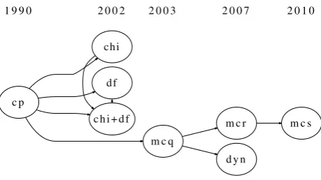
In this section we select eight BK-based algorithms and discuss them as particular variations of Algorithm MAXCLIQUEBB. The chosen algorithms, to which we will refer collectively as “MCBBalgorithms”, are the following. cp: the algorithm MAXCLIQas described in [5].
chi: the algorithmχas described in [6]. df: the algorithm DF as described in [6].
chi+df: the algorithmχ+DF as described in [6]. mcq: the algorithmMCQas described in [17]. mcr: the algorithmMCRas described in [16]. mcs: the algorithmMCSas described in [18].
dyn: the algorithm MAXCLIQUEDYNas described in [9]. The diagram in Fig.1displays the publishing timeline for theMCBBalgorithms. An arrow in the diagram means that the author of the latter work explicitly builds upon the work of the former.
We actually implemented Algorithm MAXCLIQUEBB and the variations corresponding to each of theMCBB algo-rithms in order to effect a comparative experimental analysis of their performance under the same computational environ-ment. For details on this implementation as well as on the computational environment in which the experimental data presented were gathered, we refer the reader to Sect.5. 4.1 The basic algorithm
We begin by pointing out that Algorithm MAXCLIQUE cor-responds to the variation of Algorithm MAXCLIQUEBB where
Fig. 1 Publishing timeline of theMCBBalgorithms
pre-process(G): returns the pair(G,{(∅, V (G))}), pre-process-state(G, Q, K, C): returns the pair(Q, K), bound(G, Q, K): returns the value of|K|,
remove(K): removes (and returns) a vertex fromK, update(G, C,S, Q): returns the pair(Q,S), post-process(G, C): returns the setC.
This is the most basic variation of Algorithm MAXCLIQUEBB in the sense that each of the operations above performs trivial processing in time Θ(1). We refer to this particular variation of Algorithm MAXCLIQUEBB as the “basicalgorithm”, and include it into the collective “MCBBalgorithms”.
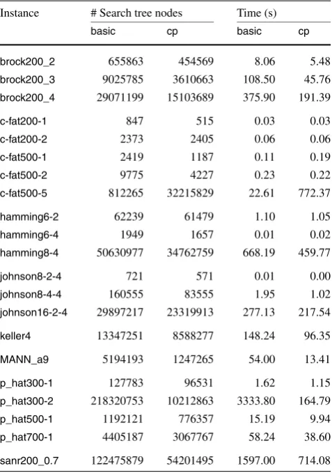
Down to implementation level, leaving the pivoting strat-egy unspecified (or underspecified) amounts to having a piv-oting strategy where the order of the vertices is induced by the data structure representing the graph. It is worth noting that the data structure representing the graph, for its turn, is sensitive to the way the input data are organized and parsed. The tables in the following sections show the number of search tree nodes and the overall execution time for thebasic algorithm confronted with the same values for executions of the otherMCBBalgorithms for 21 of theDIMACSinstances. These instances were selected because they were the ones for which each of theMCBBalgorithms ran to completion within the time limit of three hours (10800 seconds). Com-plete tables, showing these values for all of the 66DIMACS instances, are presented in theAppendix.
4.2 Non-trivial branching:cp
Among the MCBBalgorithms, cp is the first to explore a non-trivial pivoting strategy, which is to privilege low de-gree vertices as pivots. The intuitive idea behind this strat-egy is that low degree vertices are “unlikely” to be part of a maximum clique and so should be examined and discarded as soon as possible.
Table 1 Number of search tree nodes and execution time forbasicand
cp
Instance # Search tree nodes Time (s)
basic cp basic cp
brock200_2 655863 454569 8.06 5.48
brock200_3 9025785 3610663 108.50 45.76
brock200_4 29071199 15103689 375.90 191.39
c-fat200-1 847 515 0.03 0.03
c-fat200-2 2373 2405 0.06 0.06
c-fat500-1 2419 1187 0.11 0.19
c-fat500-2 9775 4227 0.23 0.22
c-fat500-5 812265 32215829 22.61 772.37
hamming6-2 62239 61479 1.10 1.05
hamming6-4 1949 1657 0.01 0.02
hamming8-4 50630977 34762759 668.19 459.77
johnson8-2-4 721 571 0.01 0.00
johnson8-4-4 160555 83555 1.95 1.02
johnson16-2-4 29897217 23319913 277.13 217.54
keller4 13347251 8588277 148.24 96.35
MANN_a9 5194193 1247265 54.00 13.41
p_hat300-1 127783 96531 1.62 1.15
p_hat300-2 218320753 10212863 3333.80 164.79
p_hat500-1 1192121 776357 15.19 9.94
p_hat700-1 4405187 3067767 58.24 38.60
sanr200_0.7 122475879 54201495 1597.00 714.08
v3 is the vertex of minimum degree in G− {v1, v2}, and so on, and remove(K) returns the lowest indexed vertex in K according to L. Moreover, if G is a “dense” graph, thenpre-process-state(G, Q, K, C)recomputes this list re-stricted toG[K]. A precise definition of “dense” is not given by the authors of [5]. In our implementation ofcpwe do not treat differently graphs according to their density leav-ingpre-process-state(G, Q, K, C)the same as in thebasic algorithm.
In Table1we show the number of search tree nodes and the overall execution time for thebasicalgorithm confronted with the same values for executions ofcpon the selected DI-MACSinstances. These values show clearly that the branch-ing strategy incpsubstantially reduces the number of search tree nodes with respect to the basic algorithm. Indeed, ex-cepting the extreme cases on both ends of the sample, we see that the number of search tree nodes for basicis 1.65 larger than the number of search tree nodes for cp (with a standard deviation of 0.43). The running times, for their turn, show clearly that the overhead imposed by the pre-processing does not compromise the overall performance of the algorithm.
A word seems to be due with respect to instance c-fat500-5, whose data seem to be so discrepant with re-spect to the otherc-fat*instances. The reason for this is the fact that the maximum clique found by the algorithm for this instance is formed by vertices of maximum degree in the graph and, as explained above, such vertices are the last ones to be considered by the algorithm. The reader will ob-serve the same phenomenon for other instances of the “c-fat* family” in theAppendix.
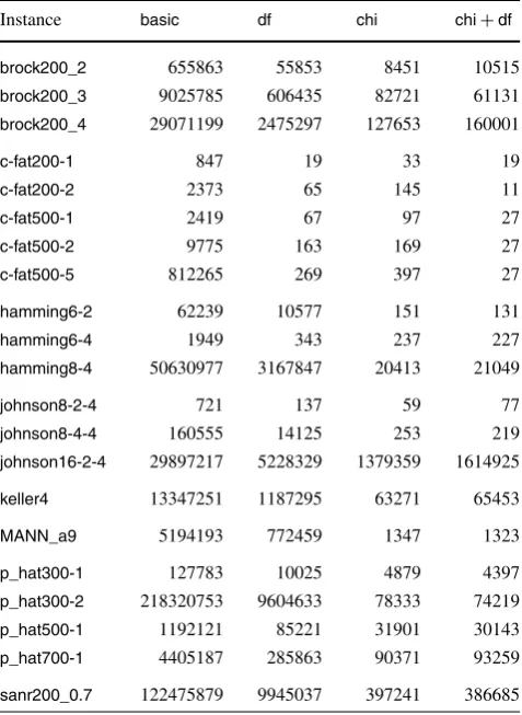
4.3 Non-trivial branching and bounding:df,chiandchi+df
Whilecpexplores the impact of a non-trivial pivoting strat-egy in the performance of maximum clique searching, the algorithmsdf,chiandchi+dfexplore the comparative im-pact of non-trivial bounding strategies. These are the first among theMCBBalgorithms to explore the idea of using an estimate on the chromatic number of the graph as an upper bound on the size of the maximum clique.
In all three of them, pre-process(G) orders V (G) into a listL=(v1, . . . , vn). No details are given by the author about this ordering, as its only purpose is to keep the ver-tices easily indexable so thatremove(K)returns the lowest indexed vertex inKaccording toL. In our implementation we use the trivialpre-process(G)of thebasicalgorithm.
In Algorithmchithe bounding step is performed by com-puting four colorings of G[K] and returning the number of colors of the one which uses the least number of col-ors. These four colorings are obtained using two different greedy coloring algorithms. Each of these coloring algo-rithms work by choosing at each step the next vertex to be colored. Different colorings are obtained by changing the policy for choosing the next vertex to be colored. As a vari-ation of Algorithm MAXCLIQUEBB, Algorithmchiis the one obtained when the routine bound(G, Q, K) performs this computation and all other custom routines are as in the basicalgorithm.
Table 2 Number of search tree nodes forbasic,chi,dfandchi+df
Instance basic df chi chi+df
brock200_2 655863 55853 8451 10515
brock200_3 9025785 606435 82721 61131
brock200_4 29071199 2475297 127653 160001
c-fat200-1 847 19 33 19
c-fat200-2 2373 65 145 11
c-fat500-1 2419 67 97 27
c-fat500-2 9775 163 169 27
c-fat500-5 812265 269 397 27
hamming6-2 62239 10577 151 131
hamming6-4 1949 343 237 227
hamming8-4 50630977 3167847 20413 21049
johnson8-2-4 721 137 59 77
johnson8-4-4 160555 14125 253 219
johnson16-2-4 29897217 5228329 1379359 1614925
keller4 13347251 1187295 63271 65453
MANN_a9 5194193 772459 1347 1323
p_hat300-1 127783 10025 4879 4397
p_hat300-2 218320753 9604633 78333 74219
p_hat500-1 1192121 85221 31901 30143
p_hat700-1 4405187 285863 90371 93259
sanr200_0.7 122475879 9945037 397241 386685
Algorithmchi+dfis simply the union of the bounding strategy of Algorithmchiand the branching strategy of Al-gorithmdfinto a single algorithm.
Table 2 shows side by side the number of search tree nodes in the execution of the same instances as in Table1.
As was the case in the discussion of algorithmcp, the val-ues for the “c-fat*family” are remarkable when compared to the others. Indeed the author of [6] himself observes that these instances “are quite easy to solve using domain filter-ing”.
Table3shows the running times corresponding to the val-ues in Table 2. Here the improvement, when there is im-provement, is much less pronounced than what one sees when comparing the number of search tree nodes. The con-clusion is that, differently from what we observed aboutcp, the overhead incurred in the more elaborate strategies of branching and bounding is not negligible and can be such as to actually increase the overall running time when compared to thebasicalgorithm. This is not completely surprising if we keep in mind the complexity of the processing which takes place at each branching and bounding step. Besides, as discussed in Sect.5, it may be the case that some of the im-plementation details contribute to make this overhead even more pronounced.
Table 3 Running time (s) forbasic,chi,dfandchi+df
Instance basic df chi chi+df
brock200_2 8.06 13.40 170.98 189.73
brock200_3 108.50 152.46 1262.22 1065.25
brock200_4 375.90 701.33 2803.73 3302.96
c-fat200-1 0.03 0.04 0.62 0.96
c-fat200-2 0.06 0.08 1.59 0.67
c-fat500-1 0.11 0.29 5.96 6.21
c-fat500-2 0.23 0.44 9.70 8.92
c-fat500-5 22.61 1.43 24.68 18.85
hamming6-2 1.10 6.26 0.72 0.99
hamming6-4 0.01 0.06 0.81 0.72
hamming8-4 668.19 973.37 1172.32 1244.42
johnson8-2-4 0.01 0.01 0.11 0.14
johnson8-4-4 1.95 2.93 2.87 2.99
johnson16-2-4 277.13 363.29 4068.67 4460.17
keller4 148.24 192.10 958.69 984.13
MANN_a9 54.00 66.18 9.19 9.35
p_hat300-1 1.62 2.58 103.97 103.22
p_hat300-2 3333.80 5108.47 4018.11 3976.74
p_hat500-1 15.19 26.16 1088.94 1022.10
p_hat700-1 58.24 95.80 3922.90 3934.76
sanr200_0.7 1597.00 3003.31 8052.30 8458.74
As we shall see in the sequel, there are ways to benefit from the idea of coloring-based bounding at a less demand-ing cost in execution time.
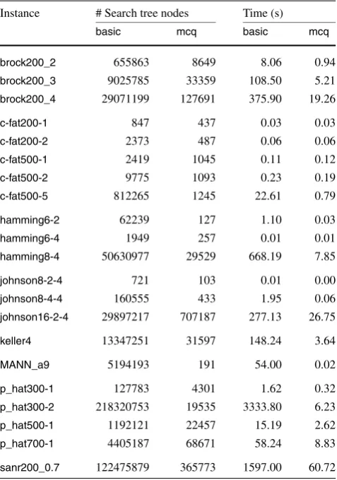
4.4 Color-based branching and bounding:mcq,mcr,mcs anddyn
The algorithms discussed above (among others) showed ex-perimental evidence that the use of non-trivial branching and bounding strategies were worth the processing time over-head per node of the search tree.
The algorithmmcqgoes one step further, using the idea of coloring the vertices of the graph not only as a bounding strategy but also as a branching strategy. The idea is that the coloring of the graph will not only provide a bound on the size of the maximum clique, but also serve as an ordering of the vertices guiding the choice of the pivot at each branching step.
Table 4 Number of search tree nodes and execution time forbasicand
mcq
Instance # Search tree nodes Time (s)
basic mcq basic mcq
brock200_2 655863 8649 8.06 0.94
brock200_3 9025785 33359 108.50 5.21
brock200_4 29071199 127691 375.90 19.26
c-fat200-1 847 437 0.03 0.03
c-fat200-2 2373 487 0.06 0.06
c-fat500-1 2419 1045 0.11 0.12
c-fat500-2 9775 1093 0.23 0.19
c-fat500-5 812265 1245 22.61 0.79
hamming6-2 62239 127 1.10 0.03
hamming6-4 1949 257 0.01 0.01
hamming8-4 50630977 29529 668.19 7.85
johnson8-2-4 721 103 0.01 0.00
johnson8-4-4 160555 433 1.95 0.06
johnson16-2-4 29897217 707187 277.13 26.75
keller4 13347251 31597 148.24 3.64
MANN_a9 5194193 191 54.00 0.02
p_hat300-1 127783 4301 1.62 0.32
p_hat300-2 218320753 19535 3333.80 6.23
p_hat500-1 1192121 22457 15.19 2.62
p_hat700-1 4405187 68671 58.24 8.83
sanr200_0.7 122475879 365773 1597.00 60.72
The routine remove(K) returns a vertex of maximum color from this coloring and the routine bound(G, Q, K) just returns the number of colors in this coloring. All other custom routines are as in thebasicalgorithm.
There are two noteworthy differences in the use of color-ing inmcqwith respect to algorithmschiandchi+df. First, only one coloring is computed at each branching step, in-stead of the four in algorithmschiandchi+df. Second, the way the pivot is chosen at the branching step is such that the coloring does not need to be recomputed for the right child of each node. As the pivotvis chosen so that it is col-ored with the maximum color inK and has a neighbor of each color less than its own color, this coloring restricted to K− {v}preserves these properties.
Table4 shows the number of search tree nodes and the overall execution time for the basic algorithm confronted with the same values for executions ofmcq. Differently from what happens with algorithmschi,dfandchi+df, the reduc-ing of the number of search tree nodes reflects directly in the running time, and the differences are even more pronounced. The algorithmsmcr,mcsanddynare improvements on mcq. The first two are proposed by some of the same authors ofmcq.
The only difference betweenmcqandmcris in the pre-processing of the graph, before the actual branch and bound is executed. In Algorithmmcrthe setV (G)is ordered into a listL=(v1, . . . , vn)wherevnis the vertex of minimum de-gree inG,vn−1is the vertex of minimum degree inG−{vn}, vn−2is the vertex of minimum degree inG−{vn−1, vn}, and so on. Ties are broken in such a way that ifvi−1andvihave the same degree, then the sum of the degrees of the neigh-bors ofviinG− {vi+1, . . . , vn}is less or equal than the sum of the degrees of the neighbors ofvi−1inG− {vi, . . . , vn}. Everything else proceeds as inmcq.
Algorithm mcs further improves pre-process(G) by modifying the adjacency matrix representing the graph so that the order of the neighbors of each vertex is compatible with the order of the vertices in the initial listL.
Besides that,pre-process-state(G, Q, K, C)computes a coloringγ of G[K] similar to the one computed bymcq, but with the following difference. If a vertexvhas neighbors colored with all the lowest|C|−|Q|colors, then a color with only one neighboruis searched for and the algorithm tries to recolorv anduso that both vertices stay on the lowest |C| − |Q|colors.
At the end,post-process(G, C)undoes the modification in the adjacency matrix made inpre-process(G).
In Algorithmdynthe branching step keeps track of the sizes of the setQin each node(Q, K)visited in the search tree. More precisely, the routine pre-process-state(G, Q, K, C)computes the number of nodes(Q, K)of the search tree visited so far satisfying|Q| ≤ |Q|. Whenever this num-ber is less than 2.5% of the number of search tree nodes vis-ited so far, the vertices in K are ordered into a list as the one computed inmcqand a coloring ofG[K]with the same properties as the one in the pre-processing ofmcqis recom-puted. This coloring, however, has the additional property of keeping the relative order of all vertices of color less or equal|C| − |Q|.
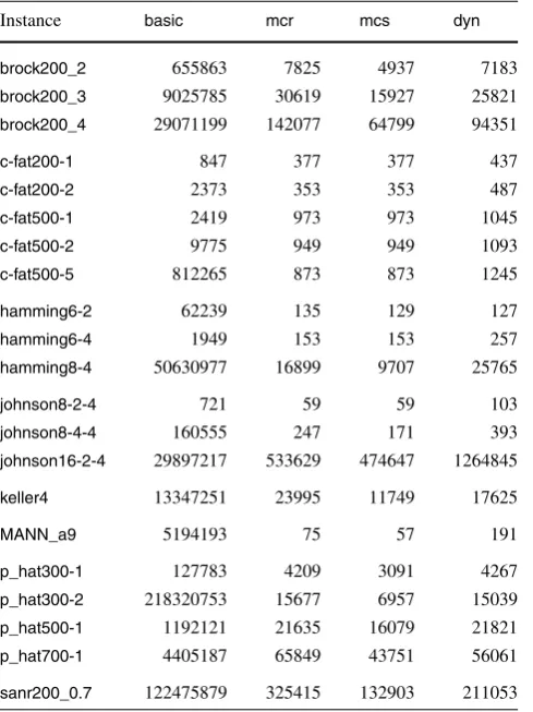
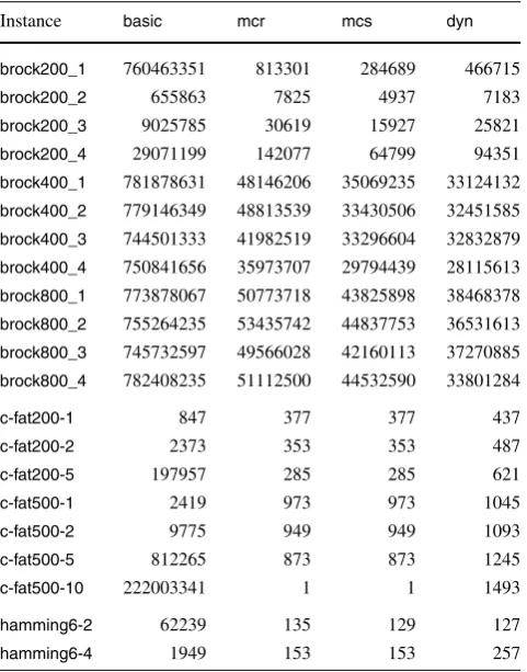
Table5shows the number of search tree nodes in the ex-ecution ofbasic,mcr,mcsanddyn. These values show that each of these algorithms effectively reduces the size of the search tree with respect tomcq.
On the other hand, differently from the observed with respect to algorithms df, chi and chi+df, the processing overhead incurred because of the non-trivial branching and bounding computation needed at each step does not cancel out the gain obtained by reducing the size of the search tree, as can be seen in Table6, which shows the running times corresponding to the entries in Table5.
Moreover, the size of the search tree formcsis further reduced with respect tomcrfor most instances. When this is not the case and both search trees have the same size, then both consume about the same processing time.
in-Table 5 Number of search tree nodes forbasic,mcr,mcsanddyn
Instance basic mcr mcs dyn
brock200_2 655863 7825 4937 7183
brock200_3 9025785 30619 15927 25821
brock200_4 29071199 142077 64799 94351
c-fat200-1 847 377 377 437
c-fat200-2 2373 353 353 487
c-fat500-1 2419 973 973 1045
c-fat500-2 9775 949 949 1093
c-fat500-5 812265 873 873 1245
hamming6-2 62239 135 129 127
hamming6-4 1949 153 153 257
hamming8-4 50630977 16899 9707 25765
johnson8-2-4 721 59 59 103
johnson8-4-4 160555 247 171 393
johnson16-2-4 29897217 533629 474647 1264845
keller4 13347251 23995 11749 17625
MANN_a9 5194193 75 57 191
p_hat300-1 127783 4209 3091 4267
p_hat300-2 218320753 15677 6957 15039
p_hat500-1 1192121 21635 16079 21821
p_hat700-1 4405187 65849 43751 56061
sanr200_0.7 122475879 325415 132903 211053
stances. This is becausemcscan be viewed as an improve-ment overmcrwhich “may or may not be triggered” depend-ing on the instance. The same is true fordynwith respect to mcq.
The conclusion is that the use of coloring as an aid for both, the branching and the bounding strategies yields al-gorithms that perform better than the ones discussed in the previous sections. This is because, (i) the coloring algorithm is simple; (ii) the choice of the pivot based on the coloring is a good pivoting strategy and (iii) colorings can be inherited and reused along some branches of the search tree.
5 Implementation details and concluding remarks
The implementation of Algorithm MAXCLIQUEBB to which our experimental results refer was made in thePython language using the framework provided by the module Net-workX. The running times were taken in aGNU/Linux sys-tem running on a 2.4 GHz, 32-core machine with 128 GB of memory. Each process was allowed to run for a maxi-mum processing time of three hours (10800 seconds). The machine was not dedicated to these experiments.
SincePythonis an interpreted language, its programs will run substantially slower than the equivalent in a compiled
Table 6 Running time (s) forbasic,mcr,mcsanddyn
Instance basic mcr mcs dyn
brock200_2 8.06 0.90 0.74 1.35
brock200_3 108.50 4.88 3.23 5.67
brock200_4 375.90 20.35 12.47 19.47
c-fat200-1 0.03 0.05 0.05 0.04
c-fat200-2 0.06 0.07 0.07 0.06
c-fat500-1 0.11 0.25 0.26 0.14
c-fat500-2 0.23 0.33 0.34 0.24
c-fat500-5 22.61 0.80 0.77 0.95
hamming6-2 1.10 0.02 0.03 0.03
hamming6-4 0.01 0.00 0.01 0.01
hamming8-4 668.19 4.64 3.03 9.47
johnson8-2-4 0.01 0.01 0.00 0.01
johnson8-4-4 1.95 0.03 0.03 0.06
johnson16-2-4 277.13 19.84 18.28 64.38
keller4 148.24 2.82 1.73 3.36
MANN_a9 54.00 0.00 0.01 0.02
p_hat300-1 1.62 0.37 0.34 0.39
p_hat300-2 3333.80 4.92 2.76 5.63
p_hat500-1 15.19 2.73 2.21 2.99
p_hat700-1 58.24 8.86 6.97 13.81
sanr200_0.7 1597.00 53.26 29.67 50.90
language. This is to note that the running times in the ex-perimental data presented are to be taken mainly as a qual-itative assessment. Indeed, implementations geared toward maximum efficiency are reported to run the same algorithms discussed here in time orders of magnitude smaller, even in computational environments less powerful than the one available here. For the purpose of this work, however, the language is very suitable in the flexibility it offers to the pro-grammer.
discus-sion of the experimental results is encouraged to refer to the respective references.
Finally, even under the limitations above pointed, the ex-perimental data presented here seem to be enough to select mcsanddynas the best algorithms forMCamong theMCBB algorithms. Indeed,mcsis the one algorithm which shows more consistently the lowest values for the number of nodes in the search tree and processing time. By a different count, however,dynis the one algorithm which solved the largest number of instances in the prescribed time, as shown in the Appendix.
Acknowledgements R. Carmo was supported by CNPq Proc. 308692/2008-0. A. Züge was partially supported by CAPES.
Appendix: Unabridged experimental data
In this appendix we present the experimental data obtained for each of theMCBB algorithms on each of theDIMACS instances.
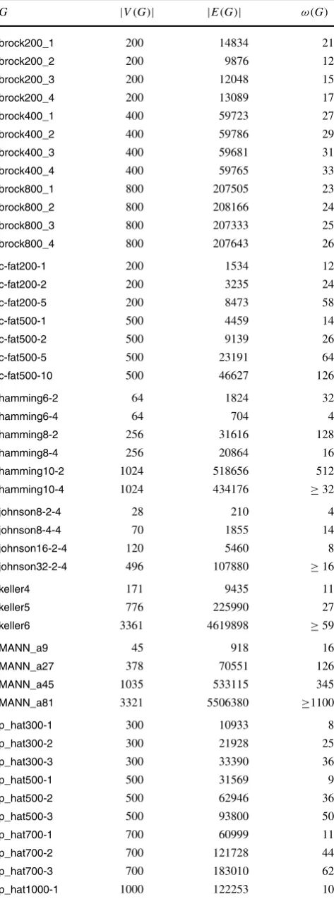
Table 7 shows the names, the number of vertices, the number of edges and the size of a maximum clique for each of the instances. Where the size of the maximum clique is shown as “≥k”, this indicates that the exact value is only known to be at leastk.
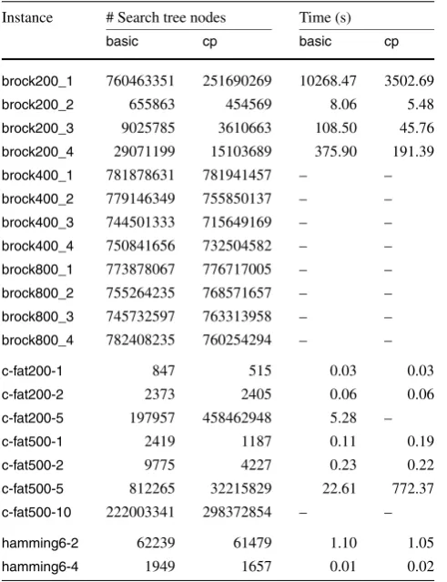
Table8 shows the number of search tree nodes and the overall execution time for the basic algorithm confronted with the same values for executions ofcp. In other words, Table8is the unabridged version of Table1.
In this and the following tables, an entry marked “–” in the column “time” means that the corresponding execution was aborted after three hours of processing (“time-out”). In such cases, the value presented as the number of search tree nodes is to be understood as the number of nodes examined up to that point in the processing.
Table9 shows the number of search tree nodes and the overall execution time for the basic algorithm confronted with the same values for executions of mcq. Table9is the unabridged version of Table4.
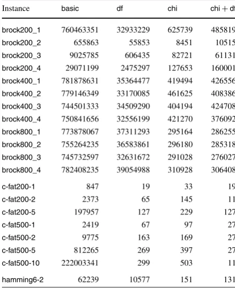
Table10shows the number of search tree nodes in the execution ofdf,chiandchi+df. Table10is the unabridged version of Table2.
Table11shows the running times in the execution ofdf, chiandchi+df. Table11is the unabridged version of Ta-ble3.
Table12shows the number of search tree nodes in the execution of basic, mcr, mcs and dyn. Table 12 is the unabridged version of Table5.
Table 13, shows the running times in the execution of basic,mcr,mcsanddyn. Table13is the unabridged version of Table6.
Table 14shows, for each of theMCBB algorithms, the average number of search tree nodes examined per second.
Table 7 Instances from the DIMACS second implementation chal-lenge
G |V (G)| |E(G)| ω(G)
brock200_1 200 14834 21
brock200_2 200 9876 12
brock200_3 200 12048 15
brock200_4 200 13089 17
brock400_1 400 59723 27
brock400_2 400 59786 29
brock400_3 400 59681 31
brock400_4 400 59765 33
brock800_1 800 207505 23
brock800_2 800 208166 24
brock800_3 800 207333 25
brock800_4 800 207643 26
c-fat200-1 200 1534 12
c-fat200-2 200 3235 24
c-fat200-5 200 8473 58
c-fat500-1 500 4459 14
c-fat500-2 500 9139 26
c-fat500-5 500 23191 64
c-fat500-10 500 46627 126
hamming6-2 64 1824 32
hamming6-4 64 704 4
hamming8-2 256 31616 128
hamming8-4 256 20864 16
hamming10-2 1024 518656 512
hamming10-4 1024 434176 ≥32
johnson8-2-4 28 210 4
johnson8-4-4 70 1855 14
johnson16-2-4 120 5460 8
johnson32-2-4 496 107880 ≥16
keller4 171 9435 11
keller5 776 225990 27
keller6 3361 4619898 ≥59
MANN_a9 45 918 16
MANN_a27 378 70551 126
MANN_a45 1035 533115 345
MANN_a81 3321 5506380 ≥1100
p_hat300-1 300 10933 8
p_hat300-2 300 21928 25
p_hat300-3 300 33390 36
p_hat500-1 500 31569 9
p_hat500-2 500 62946 36
p_hat500-3 500 93800 50
p_hat700-1 700 60999 11
p_hat700-2 700 121728 44
p_hat700-3 700 183010 62
Table 7 (Continued)
G |V (G)| |E(G)| ω(G)
p_hat1000-2 1000 244799 46
p_hat1000-3 1000 371746 68
p_hat1500-1 1500 284923 12
p_hat1500-2 1500 568960 65
p_hat1500-3 1500 847244 ≥56
san200_0.7_1 200 13930 30
san200_0.7_2 200 13930 18
san200_0.9_1 200 17910 70
san200_0.9_2 200 17910 60
san200_0.9_3 200 17910 44
san400_0.5_1 400 39900 13
san400_0.7_1 400 55860 40
san400_0.7_2 400 55860 30
san400_0.7_3 400 55860 22
san400_0.9_1 400 71820 100
san1000 1000 250500 15
sanr200_0.7 200 13868 18
sanr200_0.9 200 17863 42
sanr400_0.5 400 39984 13
sanr400_0.7 400 55869 21
Table 8 Number of search tree nodes and execution time forbasicand
cp
Instance # Search tree nodes Time (s)
basic cp basic cp
brock200_1 760463351 251690269 10268.47 3502.69
brock200_2 655863 454569 8.06 5.48
brock200_3 9025785 3610663 108.50 45.76
brock200_4 29071199 15103689 375.90 191.39
brock400_1 781878631 781941457 – –
brock400_2 779146349 755850137 – –
brock400_3 744501333 715649169 – –
brock400_4 750841656 732504582 – –
brock800_1 773878067 776717005 – –
brock800_2 755264235 768571657 – –
brock800_3 745732597 763313958 – –
brock800_4 782408235 760254294 – –
c-fat200-1 847 515 0.03 0.03
c-fat200-2 2373 2405 0.06 0.06
c-fat200-5 197957 458462948 5.28 –
c-fat500-1 2419 1187 0.11 0.19
c-fat500-2 9775 4227 0.23 0.22
c-fat500-5 812265 32215829 22.61 772.37
c-fat500-10 222003341 298372854 – –
hamming6-2 62239 61479 1.10 1.05
hamming6-4 1949 1657 0.01 0.02
Table 8 (Continued)
Instance # Search tree nodes Time (s)
basic cp basic cp
hamming8-2 479589100 352543447 – –
hamming8-4 50630977 34762759 668.19 459.77
hamming10-2 477939325 402027810 – –
hamming10-4 799627648 778850521 – –
johnson8-2-4 721 571 0.01 0.00
johnson8-4-4 160555 83555 1.95 1.02
johnson16-2-4 29897217 23319913 277.13 217.54
johnson32-2-4 1124521577 1104958353 – –
keller4 13347251 8588277 148.24 96.35
keller5 788436558 834071065 – –
keller6 814607071 779038755 – –
MANN_a9 5194193 1247265 54.00 13.41
MANN_a27 1039572148 470689919 – –
MANN_a45 896111360 293734044 – –
MANN_A81 649082104 166411314 – –
p_hat300-1 127783 96531 1.62 1.15
p_hat300-2 218320753 10212863 3333.80 164.79
p_hat300-3 694764638 632946226 – –
p_hat500-1 1192121 776357 15.19 9.94
p_hat500-2 666419883 601945642 – –
p_hat500-3 627863675 603266182 – –
p_hat700-1 4405187 3067767 58.24 38.60
p_hat700-2 674310972 570261174 – –
p_hat700-3 575688852 578871234 – –
p_hat1000-1 25084283 16177539 327.15 204.89
p_hat1000-2 651274462 589428559 – –
p_hat1000-3 609819818 546143432 – –
p_hat1500-1 232906339 139624485 3473.86 2151.07
p_hat1500-2 577460315 556716701 – –
p_hat1500-3 609271041 542561068 – –
san200_0.7_1 1199510748 1285897159 – –
san200_0.7_2 1162303528 1040102008 – –
san200_0.9_1 712616501 857295178 – –
san200_0.9_2 580762880 708916119 – –
san200_0.9_3 788583024 702721963 – –
san400_0.5_1 1057751310 1072592630 – –
san400_0.7_1 1159107699 1093205907 – –
san400_0.7_2 1091551627 1289478422 – –
san400_0.7_3 1011697883 1037906517 – –
san400_0.9_1 868327833 818891530 – –
san1000 894222972 912859488 – –
sanr200_0.7 122475879 54201495 1597.00 714.08
sanr200_0.9 708848293 626288059 – –
sanr400_0.5 53900541 36182977 680.22 457.73
Table 9 Number of search tree nodes and execution time forbasicand
mcq
Instance # Search tree nodes Time (s)
basic mcq basic mcq
brock200_1 760463351 934071 10268.47 194.72
brock200_2 655863 8649 8.06 0.94
brock200_3 9025785 33359 108.50 5.21
brock200_4 29071199 127691 375.90 19.26
brock400_1 781878631 46078511 – –
brock400_2 779146349 48936847 – –
brock400_3 744501333 40736005 – –
brock400_4 750841656 36592912 – –
brock800_1 773878067 49759405 – –
brock800_2 755264235 50923139 – –
brock800_3 745732597 49157697 – –
brock800_4 782408235 50647778 – –
c-fat200-1 847 437 0.03 0.03
c-fat200-2 2373 487 0.06 0.06
c-fat200-5 197957 621 5.28 0.31
c-fat500-1 2419 1045 0.11 0.12
c-fat500-2 9775 1093 0.23 0.19
c-fat500-5 812265 1245 22.61 0.79
c-fat500-10 222003341 1493 – 19.16
hamming6-2 62239 127 1.10 0.03
hamming6-4 1949 257 0.01 0.01
hamming8-2 479589100 519 – 1.79
hamming8-4 50630977 29529 668.19 7.85
hamming10-2 477939325 2433 – 178.36
hamming10-4 799627648 38911002 – –
johnson8-2-4 721 103 0.01 0.00
johnson8-4-4 160555 433 1.95 0.06
johnson16-2-4 29897217 707187 277.13 26.75
johnson32-2-4 1124521577 286689139 – –
keller4 13347251 31597 148.24 3.64
keller5 788436558 21418630 – –
keller6 814607071 18188831 – –
MANN_a9 5194193 191 54.00 0.02
MANN_a27 1039572148 86157 – 919.57
MANN_a45 896111360 129263 – –
MANN_A81 649082104 13107 – –
p_hat300-1 127783 4301 1.62 0.32
p_hat300-2 218320753 19535 3333.80 6.23
p_hat300-3 694764638 5122669 – 2508.94
p_hat500-1 1192121 22457 15.19 2.62
p_hat500-2 666419883 1084401 – 566.91
p_hat500-3 627863675 16142732 – –
p_hat700-1 4405187 68671 58.24 8.83
p_hat700-2 674310972 8798091 – 7296.62
p_hat700-3 575688852 11194735 – –
Table 9 (Continued)
Instance # Search tree nodes Time (s)
basic mcq basic mcq
p_hat1000-1 25084283 406251 327.15 50.43
p_hat1000-2 651274462 13673923 – –
p_hat1000-3 609819818 16712232 – –
p_hat1500-1 232906339 2567285 3473.86 442.68
p_hat1500-2 577460315 13699588 – –
p_hat1500-3 609271041 14540018 – –
san200_0.7_1 1199510748 3551 – 1.53
san200_0.7_2 1162303528 3531 – 0.72
san200_0.9_1 712616501 453207 – 214.31
san200_0.9_2 580762880 2166287 – 1315.95
san200_0.9_3 788583024 1854567 – 1450.32
san400_0.5_1 1057751310 5601 – 3.00
san400_0.7_1 1159107699 174471 – 136.18
san400_0.7_2 1091551627 134609 – 119.02
san400_0.7_3 1011697883 895391 – 383.13
san400_0.9_1 868327833 83553153 – –
san1000 894222972 511507 – 1093.09
sanr200_0.7 122475879 365773 1597.00 60.72
sanr200_0.9 708848293 19847341 – –
sanr400_0.5 53900541 610909 680.22 75.05
sanr400_0.7 791421504 48382248 – –
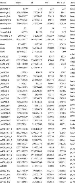
Table 10 Number of search tree nodes forbasic,chi,dfandchi+df
Instance basic df chi chi+df
brock200_1 760463351 32933229 625739 485819
brock200_2 655863 55853 8451 10515
brock200_3 9025785 606435 82721 61131
brock200_4 29071199 2475297 127653 160001
brock400_1 781878631 35364477 419494 426556
brock400_2 779146349 33170085 461625 408386
brock400_3 744501333 34509290 404194 424708
brock400_4 750841656 32556199 421270 376092
brock800_1 773878067 37311293 295164 286255
brock800_2 755264235 36583861 296180 285318
brock800_3 745732597 32631672 291028 276027
brock800_4 782408235 39054988 310928 306408
c-fat200-1 847 19 33 19
c-fat200-2 2373 65 145 11
c-fat200-5 197957 127 229 127
c-fat500-1 2419 67 97 27
c-fat500-2 9775 163 169 27
c-fat500-5 812265 269 397 27
c-fat500-10 222003341 299 503 11
Table 10 (Continued)
Instance basic df chi chi+df
hamming6-4 1949 343 237 227
hamming8-2 479589100 7705015 3973 1841
hamming8-4 50630977 3167847 20413 21049
hamming10-2 477939325 24989216 15841 15880
hamming10-4 799627648 34293269 147962 100629
johnson8-2-4 721 137 59 77
johnson8-4-4 160555 14125 253 219
johnson16-2-4 29897217 5228329 1379359 1614925
johnson32-2-4 1124521577 163763590 2158150 2374215
keller4 13347251 1187295 63271 65453
keller5 788436558 36800640 152609 158865
keller6 814607071 31790821 933 790
MANN_a9 5194193 772459 1347 1323
MANN_a27 1039572148 276077527 45063 73981
MANN_a45 896111360 247828444 2585 2332
MANN_A81 649082104 134484013 18 15
p_hat300-1 127783 10025 4879 4397
p_hat300-2 218320753 9604633 78333 74219
p_hat300-3 694764638 25445287 257474 267335
p_hat500-1 1192121 85221 31901 30143
p_hat500-2 666419883 19861603 168191 156518
p_hat500-3 627863675 26495825 148979 197406
p_hat700-1 4405187 285863 90371 93259
p_hat700-2 674310972 19704073 150286 124285
p_hat700-3 575688852 21204840 82150 115173
p_hat1000-1 25084283 1688731 273593 287859
p_hat1000-2 651274462 22031073 132626 142135
p_hat1000-3 609819818 20670410 90971 100185
p_hat1500-1 232906339 13776857 179966 186962
p_hat1500-2 577460315 21490388 60226 68721
p_hat1500-3 609271041 21103903 69038 44671
san200_0.7_1 1199510748 230612837 35959 999
san200_0.7_2 1162303528 139202470 20719 20585
san200_0.9_1 712616501 95545497 160730 189882
san200_0.9_2 580762880 22944996 58131 184741
san200_0.9_3 788583024 30003374 413304 371226
san400_0.5_1 1057751310 83927533 4029 3081
san400_0.7_1 1159107699 293738048 108630 173528
san400_0.7_2 1091551627 191488689 240064 200279
san400_0.7_3 1011697883 173777224 438690 243408
san400_0.9_1 868327833 106086764 104439 398631
san1000 894222972 31153745 20004 20194
sanr200_0.7 122475879 9945037 397241 386685
sanr200_0.9 708848293 33205279 360044 339146
sanr400_0.5 53900541 4214565 558533 544368
sanr400_0.7 791421504 36721656 432554 454927
Table 11 Running time (s) forbasic,chi,dfandchi+df
Instance basic df chi chi+df
brock200_1 10268.47 – – –
brock200_2 8.06 13.40 170.98 189.73
brock200_3 108.50 152.46 1262.22 1065.25
brock200_4 375.90 701.33 2803.73 3302.96
brock400_1 – – – –
brock400_2 – – – –
brock400_3 – – – –
brock400_4 – – – –
brock800_1 – – – –
brock800_2 – – – –
brock800_3 – – – –
brock800_4 – – – –
c-fat200-1 0.03 0.04 0.62 0.96
c-fat200-2 0.06 0.08 1.59 0.67
c-fat200-5 5.28 0.43 22.05 21.26
c-fat500-1 0.11 0.29 5.96 6.21
c-fat500-2 0.23 0.44 9.70 8.92
c-fat500-5 22.61 1.43 24.68 18.85
c-fat500-10 – 11.91 94.35 10.00
hamming6-2 1.10 6.26 0.72 0.99
hamming6-4 0.01 0.06 0.81 0.72
hamming8-2 – – 541.34 531.47
hamming8-4 668.19 973.37 1172.32 1244.42
hamming10-2 – – – –
hamming10-4 – – – –
johnson8-2-4 0.01 0.01 0.11 0.14
johnson8-4-4 1.95 2.93 2.87 2.99
johnson16-2-4 277.13 363.29 4068.67 4460.17
johnson32-2-4 – – – –
keller4 148.24 192.10 958.69 984.13
keller5 – – – –
keller6 – – – –
MANN_a9 54 66.18 9.19 9.35
MANN_a27 – – – –
MANN_a45 – – – –
MANN_A81 – – – –
p_hat300-1 1.62 2.58 103.97 103.22
p_hat300-2 3333.80 5108.47 4018.11 3976.74
p_hat300-3 – – – –
p_hat500-1 15.19 26.16 1088.94 1022.10
p_hat500-2 – – – –
p_hat500-3 – – – –
p_hat700-1 58.24 95.80 3922.90 3934.76
p_hat700-2 – – – –
p_hat700-3 – – – –
Table 11 (Continued)
Instance basic df chi chi+df
p_hat1000-2 – – – –
p_hat1000-3 – – – –
p_hat1500-1 3473.86 5638.03 – –
p_hat1500-2 – – – –
p_hat1500-3 – – – –
san200_0.7_1 – – 968.54 41.62
san200_0.7_2 – – 686.48 1005.41
san200_0.9_1 – – – –
san200_0.9_2 – – 6522.12 –
san200_0.9_3 – – – –
san400_0.5_1 – – 276.68 198.35
san400_0.7_1 – – – –
san400_0.7_2 – – – –
san400_0.7_3 – – – –
san400_0.9_1 – – – –
san1000 – – – –
sanr200_0.7 1597 3003.31 8052.30 8458.74
sanr200_0.9 – – – –
sanr400_0.5 680.22 1050.91 – –
sanr400_0.7 – – – –
Table 12 Number of search tree nodes forbasic,mcr,mcsanddyn
Instance basic mcr mcs dyn
brock200_1 760463351 813301 284689 466715
brock200_2 655863 7825 4937 7183
brock200_3 9025785 30619 15927 25821
brock200_4 29071199 142077 64799 94351
brock400_1 781878631 48146206 35069235 33124132
brock400_2 779146349 48813539 33430506 32451585
brock400_3 744501333 41982519 33296604 32832879
brock400_4 750841656 35973707 29794439 28115613
brock800_1 773878067 50773718 43825898 38468378
brock800_2 755264235 53435742 44837753 36531613
brock800_3 745732597 49566028 42160113 37270885
brock800_4 782408235 51112500 44532590 33801284
c-fat200-1 847 377 377 437
c-fat200-2 2373 353 353 487
c-fat200-5 197957 285 285 621
c-fat500-1 2419 973 973 1045
c-fat500-2 9775 949 949 1093
c-fat500-5 812265 873 873 1245
c-fat500-10 222003341 1 1 1493
hamming6-2 62239 135 129 127
hamming6-4 1949 153 153 257
Table 12 (Continued)
Instance basic mcr mcs dyn
hamming8-2 479589100 1207 1057 537
hamming8-4 50630977 16899 9707 25765
hamming10-2 477939325 23141 2497 2167
hamming10-4 799627648 37220492 15618125 19888977
johnson8-2-4 721 59 59 103
johnson8-4-4 160555 247 171 393
johnson16-2-4 29897217 533629 474647 1264845
johnson32-2-4 1124521577 288086577 282675611 236697572
keller4 13347251 23995 11749 17625
keller5 788436558 16911848 17475952 13452717
keller6 814607071 13800894 16179301 6555099
MANN_a9 5194193 75 57 191
MANN_a27 1039572148 29763 7615 86157
MANN_a45 896111360 129059 164086 94849
MANN_A81 649082104 12942 12942 9555
p_hat300-1 127783 4209 3091 4267
p_hat300-2 218320753 15677 6957 15039
p_hat300-3 694764638 3103461 523957 1257961
p_hat500-1 1192121 21635 16079 21821
p_hat500-2 666419883 627809 137045 379719
p_hat500-3 627863675 15527986 7860621 7118821
p_hat700-1 4405187 65849 43751 56061
p_hat700-2 674310972 5583275 700379 2195677
p_hat700-3 575688852 10991858 6126902 5211837
p_hat1000-1 25084283 398281 234723 339555
p_hat1000-2 651274462 12990532 8868752 7810188
p_hat1000-3 609819818 16924970 7386341 6864282
p_hat1500-1 232906339 2481911 1564723 2277359
p_hat1500-2 577460315 12680238 6257860 6025488
p_hat1500-3 609271041 14830728 4880291 5044208
san200_0.7_1 1199510748 7779 1739 2103
san200_0.7_2 1162303528 3145 1537 4603
san200_0.9_1 712616501 456721 47993 77603
san200_0.9_2 580762880 717197 26629 586527
san200_0.9_3 788583024 126665 7039 585453
san400_0.5_1 1057751310 4719 3023 4811
san400_0.7_1 1159107699 217471 48269 90853
san400_0.7_2 1091551627 42627 26811 18985
san400_0.7_3 1011697883 810445 248085 763393
san400_0.9_1 868327833 16184155 9529297 766201
san1000 894222972 426757 168419 251773
sanr200_0.7 122475879 325415 132903 211053
sanr200_0.9 708848293 19698991 6130061 12709733
sanr400_0.5 53900541 586913 329631 509701
Table 13 Running time (s) forbasic,mcr,mcsanddyn
Instance basic mcr mcs dyn
brock200_1 10268.47 168.36 79.72 140.60
brock200_2 8.06 0.90 0.74 1.35
brock200_3 108.50 4.88 3.23 5.67
brock200_4 375.90 20.35 12.47 19.47
brock400_1 – – – –
brock400_2 – – – –
brock400_3 – – – –
brock400_4 – – – –
brock800_1 – – – –
brock800_2 – – – –
brock800_3 – – – –
brock800_4 – – – –
c-fat200-1 0.03 0.05 0.05 0.04
c-fat200-2 0.06 0.07 0.07 0.06
c-fat200-5 5.28 0.21 0.21 0.36
c-fat500-1 0.11 0.25 0.26 0.14
c-fat500-2 0.23 0.33 0.34 0.24
c-fat500-5 22.61 0.80 0.77 0.95
c-fat500-10 – 1.57 0.68 10.29
hamming6-2 1.10 0.02 0.03 0.03
hamming6-4 0.01 0.00 0.01 0.01
hamming8-2 – 4.24 4.67 2.46
hamming8-4 668.19 4.64 3.03 9.47
hamming10-2 – 3269.93 190.30 195.95
hamming10-4 – – – –
johnson8-2-4 0.01 0.01 0.00 0.01
johnson8-4-4 1.95 0.03 0.03 0.06
johnson16-2-4 277.13 19.84 18.28 64.38
johnson32-2-4 – – – –
keller4 148.24 2.82 1.73 3.36
keller5 – – – –
keller6 – – – –
MANN_a9 54.00 0.00 0.01 0.02
MANN_a27 – 302.00 63.32 1280.38
MANN_a45 – – – –
MANN_A81 – – – –
p_hat300-1 1.62 0.37 0.34 0.39
p_hat300-2 3333.80 4.92 2.76 5.63
p_hat300-3 – 1586.09 366.70 951.82
p_hat500-1 15.19 2.73 2.21 2.99
p_hat500-2 – 349.39 94.19 281.62
p_hat500-3 – – – –
p_hat700-1 58.24 8.86 6.97 13.81
p_hat700-2 – 4743.96 763.28 2637.62
p_hat700-3 – – – –
p_hat1000-1 327.15 49.21 34.61 66.25
Table 13 (Continued)
Instance basic mcr mcs dyn
p_hat1000-2 – – – –
p_hat1000-3 – – – –
p_hat1500-1 3473.86 428.89 274.09 529.73
p_hat1500-2 – – – –
p_hat1500-3 – – – –
san200_0.7_1 – 2.51 0.82 1.24
san200_0.7_2 – 0.63 0.41 1.46
san200_0.9_1 – 206.17 35.23 68.44
san200_0.9_2 – 391.74 23.37 581.02
san200_0.9_3 – 43.70 4.72 691.17
san400_0.5_1 – 2.79 1.79 2.28
san400_0.7_1 – 212.86 50.85 75.95
san400_0.7_2 – 30.13 15.67 26.69
san400_0.7_3 – 356.42 110.19 293.37
san400_0.9_1 – – – 4906.83
san1000 – 910.12 298.10 147.11
sanr200_0.7 1597.00 53.26 29.67 50.90
sanr200_0.9 – – 5223.79 10692.55
sanr400_0.5 680.22 72.19 51.47 83.51
sanr400_0.7 – – – –
Table 14 Average search tree node per second and number of solved instances for each algorithm
Algorithm (# Search tree nodes)/s Solved instances
basic 72066.01 26
cp 66490.03 25
df 6648.27 26
chi 28.87 28
chi+df 29.58 27
mcq 3778.20 43
dyn 2579.93 45
mcr 3523.45 43
mcs 3014.30 44
This is the number of search tree nodes summed over all the instances, divided by the total time summed over all the in-stances. The last column shows how many of the instances were solved to completion within the prescribed time of three hours.
References
2. Bollobás B (2001) Random graphs. Cambridge University Press, Cambridge. http://books.google.com/books?hl=en&lr=&id= o9WecWgilzYC&oi=fnd&pg=PR10&dq=
bollobas%2Brandom%2Bgraphs&ots=YyFTnSQpVh&sig= 7GrvDOb_MJLesgbjLvQj0TeNG8U#PPP1,M1
3. Bomze IM, Budinich M, Pardalos PM, Pelillo M (1999) The maximum clique problem. In: Handbook of combinatorial op-timization, vol 4, pp 1–74. http://citeseerx.ist.psu.edu/viewdoc/ summary?doi=10.1.1.56.6221
4. Bron C, Kerbosch J (1973) Algorithm 457: finding all cliques of an undirected graph. Commun ACM 16(9):575–577. doi:10.1145/ 362342.362367
5. Carraghan R, Pardalos PM (1990) An exact algorithm for the maximum clique problem. Oper Res Lett9(6). doi: 10.1016/0167-6377(90)90057-C
6. Fahle T (2002) Simple and fast: Improving a branch-and-bound algorithm for maximum clique. In: Lecture notes in computer sci-ence. Springer, Berlin, pp 47–86. doi:10.1007/3-540-45749-6_44 7. Garey M, Johnson D (1979) Computers and intractability.
Free-man, San Francisco
8. Jian T (1986) Ano(20.304n)algorithm for solving maximum
inde-pendent set problem. IEEE Trans Comput 35(9):847–851. doi:10. 1109/TC.1986.1676847
9. Konc J, Janezic D (2007) An improved branch and bound algo-rithm for the maximum clique problem. MATCH Commun Math Comput Chem. http://www.sicmm.org/~konc/%C4%8CLANKI/ MATCH58(3)569-590.pdf
10. Li CM, Quan Z (2010) An efficient branch-and-bound algorithm based on maxsat for the maximum clique problem. In: Twenty-fourth AAAI conference on artificial intelligence. http://www. aaai.org/ocs/index.php/AAAI/AAAI10/paper/view/1611
11. Moon J, Moser L (1965) On cliques in graphs. Isr J Math 3(1):23– 28. doi:10.1007/BF02760024
12. Östergård PR (2002) A fast algorithm for the maximum clique problem. Discrete Appl Math 120(1–3):197–207. doi:10.1016/ S0166-218X(01)00290-6
13. Robson J (1986) Algorithms for maximum independent sets. J Al-gorithms 7(3):425–440. doi:10.1016/0196-6774(86)90032-5 14. Robson J (2001) Finding a maximum independent set in time
o(2(n/4)).http://www.labri.fr/perso/robson/mis/techrep.html
15. Tarjan RE, Trojanowski AE (1976) Finding a maximum indepen-dent set. Tech. rep., Computer Science Department, School of Hu-manities and Sciences, Stanford University, Stanford, CA, USA. http://portal.acm.org/citation.cfm?id=892099
16. Tomita E, Kameda T (2007) An efficient branch-and-bound al-gorithm for finding a maximum clique with computational ex-periments. J Glob Optim 37(1):95–111. doi: 10.1007/s10898-006-9039-7
17. Tomita E, Seki T (2003) An efficient branch-and-bound algo-rithm for finding a maximum clique. Springer, Berlin.http://www. springerlink.com/content/7jbjyglyqc8ca5n9
18. Tomita E, Sutani Y, Higashi T, Takahashi S, Wakatsuki M (2010) A simple and faster branch-and-bound algorithm for finding a maximum clique. In: Rahman M, Fujita S (eds) WALCOM: Algo-rithms and computation, vol 5942. Springer, Berlin, pp 191–203. doi:10.1007/978-3-642-11440-3_18. Chap. 18