DOI 10.1007/s13173-013-0107-9 O R I G I NA L PA P E R
Terminating constraint set satisfiability and simplification
algorithms for context-dependent overloading
Rodrigo Ribeiro · Carlos Camarão · Lucília Figueiredo
Received: 24 August 2012 / Accepted: 4 March 2013 / Published online: 9 April 2013 © The Brazilian Computer Society 2013
Abstract Algorithms for constraint set satisfiability and simplification of Haskell type class constraints are used dur-ing type inference in order to allow the inference of more accurate types and to detect ambiguity. Unfortunately, both constraint set satisfiability and simplification are in general undecidable, and the use of these algorithms may cause non-termination of type inference. This paper presents algorithms for these problems that terminate on any given input, based on the use of a criterion that is tested on each recursive step. The use of this criterion eliminates the need of imposing syntactic conditions on Haskell type class and instance declarations in order to guarantee termination of type inference in the pres-ence of multi-parameter type classes, and allows program compilation without the need of compiler flags for lifting such restrictions. Undecidability of the problems implies the existence of instances for which the algorithm incorrectly reports unsatisfiability, but we are not aware of any practical example where this occurs.
Keywords Haskell · Constraint set satisfiability · Constraint set simplification·Termination
R. Ribeiro (
B
)·C. CamarãoInstituto de Ciências Exatas, Departamento de Ciência da Computação, Universidade Federal de Minas Gerais, Belo Horizonte, Brazil
e-mail: [email protected] C. Camarão
e-mail: [email protected] L. Figueiredo
Instituto de Ciências Exatas e Biológicas, Departamento de Computação,
Universidade Federal de Ouro Preto, Ouro Preto, Brazil e-mail: [email protected]
1 Introduction
Haskell’s type class system [5,18] extends the Hindley-Milner type system [16] with constrained polymorphic types, in order to support overloading. Type class constraints may occur in types of expressions involving overloaded names (or symbols), and restrict the set of types to which quanti-fied type variables may be instantiated, to those types for which these type constraints are satisfied, according to types of definitions that exist in a relevant context.
A type class declaration specifies the name and parameters of the class, and the principal type of names which can then be overloaded in instance definitions. For example:
class Eq a where
(==):: a → a → Bool
(/=):: a → a → Bool
is a declaration of type classEq, with parametera, that spec-ifies the principal types of(==)and(/=). Function(==) has type∀a.Eq a ⇒a →a →Bool, where constraintEq a indicates that type variablea cannot be instantiated to an arbitrary type, but only to a type that has been defined as an instance of classEq.
An instance of a type class specifies instance types for type class parameters, and gives definitions of the overloaded names specified in the class. The type of each overloaded name in an instance definition is obtained by substituting type class parameters with corresponding instance types. For example, the following instance declarations specify defini-tions of the equality operator for typesIntand for polymor-phic lists, respectively:
instance Eq a ⇒ Eq [a] where
[ ] == [ ] = True
(a:x) == (b:y) = a == b && x == y
_ == _ = False
For a base type, likeInt, a corresponding predefined oper-ation is provided. The definition of equality for lists of ele-ments of an arbitrary type uses the equality test for eleele-ments of this type. ConstraintEq amust be specified as thecontext
for thehead Eq[a]of the instance declaration. Acontextis a set of type class constraints, and constraintπis theheadof a qualified constraintP⇒π, wherePis a set of type class constraints.
As an aside, type classes in Haskell may also contain default definitions of the overloaded names, in order to avoid repeating the same definitions in instances.
Class constraints introduced on the types of overloaded symbols occur also on the types of expressions defined in terms of these symbols. For example, consider the following function that tests list membership:
elem a [ ] = False
elem a (b:x) = a == b || elem a x
The principal type ofelem is∀a.Eq a ⇒ a → [a] → Bool. ConstraintEq aoccurs in the type ofelemdue to the use of the equality operator(==)in its definition.
Haskell restricts type classes to have a single parame-ter but the extension to multi-parameparame-ter type classes, called Haskell+mptcs in the sequel, is widely used.
Type inference for constrained type systems rely on con-straint set simplification, which, for the case of type classes, essentially amounts to performing (so-called)context reduc-tion. Constraint set simplification yields equivalent constraint sets, and are useful for providing simpler types for expres-sions. Context reduction simplifies constraints by substitut-ing constraints or removsubstitut-ing resolved constraints accordsubstitut-ing to available instance definitions, besides removing duplicate constraints or substituting constraints according to the class hierarchy.
As an example, context Eq[t] is reduced toEq t, for any typet, in the presence of instanceEq[a]with context
Eq a.
Improvement [13] is also a process of simplification of constrained types, but it is of a different nature, and is used in type inference to avoid ambiguity and to infer more informa-tive types. Improvement is fundamentally based on constraint set satisfiability: it is a process of transforming a constraint setPinto a constraint set obtained by applying a substitution
StoPso that the set of satisfiable instances ofPis preserved. The mechanism of functional dependencies and other alternatives have been proposed to deal with improvement [7,4,10,11,14], for detection of ambiguity and for
specializa-tion of constrained types in the presence of multi-parameter type classes. We do not discuss improvement specifically in this paper, but focus on constraint set satisfiability, which is only used for the implementation of improvement or any alternative approach.
Unfortunately, both constraint set satisfiability and sim-plification are in general undecidable problems [6], and the use of computable functions for solving these problems may cause non-termination of type inference.
This paper presents algorithms for constraint set satis-fiability and simplification that use a termination criterion which is based on a measure of the sizes of types in type constraints. The sequence of constraints that unify with a constraint axiom in recursive calls of the function that checks satisfiability or simplification of a type constraint is such that either the sizes of types of each constraint in this sequence is decreasing or there exists at least one type parameter position with decreasing size.
The use of this criterion eliminates the need for imposing syntactic conditions on Haskell type class and instance dec-larations in order to guarantee termination of type inference in the presence of multi-parameter type classes, and allows program compilation without the need of compiler flags for lifting such restrictions.
The use of a termination criterion implies that there exist well-typed programs for which the presented algorithm incorrectly reports unsatisfiability. However, practical exam-ples where this occurs are expected to be very rare. The algorithms have been implemented and tested by using a prototype front-end for Haskell, available at the mptc github repository. The algorithm works as expected when subjected to examples mentioned in the literature, Haskell libraries that use multi-parameter type classes and many tests, including those used by the most commonly used Haskell compiler [19], GHC, involving all pertinent GHC extensions.
Restrictions imposed on class and instance declarations in Haskell, in Haskell+mptcs and in GHC, and GHC com-pilation flags used to avoid these restrictions [20], are sum-marized in Sect.2. Section3reviews entailment and satis-fiability relations on type class constraints. Section4gives a definition of a computable function that returns the set of satisfiable substitutions of a given constraint set P, when it terminates. Subsection4.1defines a termination criterion and redefines this computable function in order to use this crite-rion. Section5defines a constraint set simplification com-putable function, based on the same termination criterion. Section6concludes.
2 Restrictions over class and instance declarations
GHC, and GHC compilation flags used to avoid these restric-tions.
By default, GHC follows the Haskell language specifi-cation (i.e., the Haskell 98 report [8]), which imposes the following restrictions.
1. Each class declaration must have exactly one parameter. 2. The head of a qualified constraint in an instance declara-tion must have the formC(Tα), whereCdenotes a class name,T a type constructor andαa sequence of distinct type variables. Such overbar notation is used extensively in this paper: x denotes a possibly empty sequence of elements in the set{x1, . . . ,xn}, for somen ≥0.
3. Each constraint in a contextPof an instance declaration
P ⇒ Cτ must have the form C a, wherea is a type variable occurring inτ.
Restriction 1 allows only single-parameter type classes, but multi-parameter type classes are widely used by pro-grammers and in Haskell libraries and are supported in many Haskell implementations. For example, consider type class
Mapparameterized by the key and element types, and the type classCollection, parameterized by the type constructor and the type of elements of the collection, partly sketched below:
class Eq a ⇒ Collection c a where
empty:: c a
insert, delete:: a -> c a -> c a member:: a -> c a -> Bool
…
instanceShow(Tree Int)where …is an example of an instance declaration that does not follow restriction (2), because the head of the constraint (which has an empty con-text) consists of type constructorTreeapplied toInt, not to a type variable.
Flag-XFlexibleInstances can be used by GHC users to avoid enforcing condition (2), i.e., to allow the head of a constraint in an instance declaration to be arbitrarily nested. The next is an example that does not follow restriction (3), sinces ais not just a type variable:instanceShow
(s a)⇒Show(Sized s a)...
Instances that do not follow these restrictions are com-mon in Haskell programs, specially in the presence of multi-parameter type classes.
Flag-XFlexibleContextscan be used by GHC users to avoid restriction (3). With the use of this flag, contexts are restricted as follows:
1. No type variable can have more occurrences in a con-straint of a context than in the head.
2. The sum of the number ofoccurrencesof type variables and type constructors in a context must be smaller than in the head.
This restriction is known as the Paterson Condition. In some cases, it is still over-restrictive. As an example, consider the following code:
data Rose f a = Rose (f (Rose f a))
instance (Show (f (Rose f a)), Show a) ⇒
Show (Rose f a) where ... This instance ofShowis rejected by GHC because it has more occurrences of type variable f in a constraint than in the head. Flag-XUndecidableInstances, which lifts all restrictions (including those related to the use of func-tional dependencies), is needed to compile this code. With this flag, termination is ensured by imposing a depth limit on a recursion stack [20].
3 Constrained polymorphism and type class constraints
The Haskell type class system is based on the more general theory ofqualified types [12], which extends the Hindley-Milner type system with constrained types.
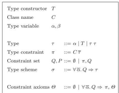
The syntax of types with type class constraints is defined in Fig. 1, where meta-variable usage is also indicated. For simplicity, and following common practice, kinds are not considered explicitly in type expressions, and type applica-tions are assumed to be well kinded. Function typesτ1→τ2 are constructed as the curried application of the function type constructor to two arguments, and are written as usual in infix notation.
The union of constraint sets PandQis denoted byP,Q
and a slight abuse of notation is made by writing simplyπ for the singleton constraint set{π}.
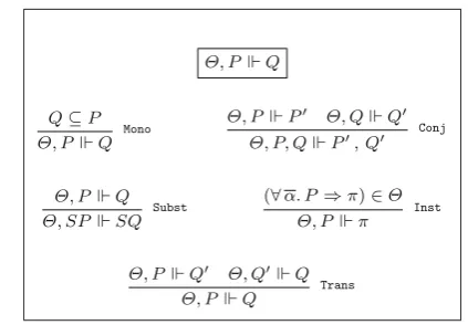
Fig. 2 Type class constraint entailment
Functiontvis overloaded, yielding the set of free type vari-ables of types, constraints or constraint sets, and is defined as usual. Sequenceαused in the context of a set denotes of course the set of type variables in the sequence. The set of constraint axiomsis induced by class and instance decla-rations of a program. Each instance declarationinstance
P⇒πwhere …introduces an axiom scheme∀α.P ⇒π, whereα=tv(P⇒π).
For simplicity and to avoid clutter, in this paper constraint axioms introduced by type class declarations are not consid-ered, since they add no additional problems with respect to termination of constraint set satisfiability and simplification algorithms.
The entailment relation for type class constraints is defined in Fig.2. Rule (Mono) expresses the property of monotonic-ity, (Trans) of transitivmonotonic-ity, (Subst) of closure under type substitution (cf. [12]), (Inst) defines entailment according to a constraint axiom and (Conj) deals with sets with more than one constraint.
A type substitutionSis a (kind-preserving) function from type variables to types, and extends straightforwardly to straints, and to sets of types and sets of constraints. For con-venience, a substitution is often written as a finite mapping [α1 → τ1, . . . , αn → τn], which is also abbreviated as
[α→τ]. JuxtapositionSSis used as a synonym for func-tion composifunc-tion,S◦ S, the domain of a substitution S is defined bydom(S)= {α| S(α) =α}and the restriction of
StoV is given byS|V(α)=S(α)ifα∈V, otherwiseα.
3.1 Constraint set satisfiability
Constraint set satisfiability is central to the interpretation of constrained types and is closely related to simplification and improvement. Following [13],Pdenotes the set of satis-fiable instances of constraint setP, with respect to constraint axioms:
P = {S P | S P}
Equality of constraint sets is considered modulo type vari-able renaming. That is, constraint sets PandQare consid-ered to be equal by considering also that a renaming sub-stitution S can be applied to P so as to make S P and Q
equal. A substitution S is a renaming substitution if for all
α∈dom(S)we have thatS(α)=β, for some type variable
β ∈dom(S).
If S P ∈ P thenS is called a satisfying substitution for P.
Subscript will not be used hereafter because satisfia-bility is always considered with respect to a set of global constraint axioms.
For any substitution Sand constraint set Pwe have that
S P ⊆ P. The reverse inclusion, P ⊆ S P, does not always hold, and allow us to characterize improvement of the set of constraints P to an equivalent but simpler or more informative constraint setS P, such thatS P = P. Substitution S is called an improving substitution for P if applying S to P preserves the set of satisfiable instances, that is, ifS P = P.
The next section presents constraint set satisfiability algo-rithms, including an algorithm that uses a criterion for guar-anteeing termination on any given input. This termination criterion is used in Sect.5, to define a constraint set simpli-fication algorithm.
4 Computing constraint set satisfiability
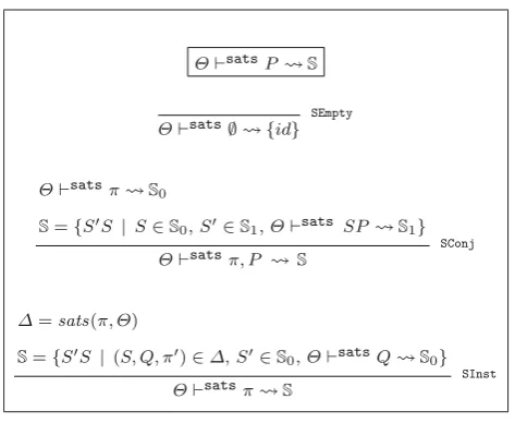
Figure3presents a computable function that, given any con-straint set P, returns, if it terminates, the set of satisfying substitutions for P. The definition uses judgements of the formsats
PS, meaning thatSis the set of satisfying substitutions forP, with respect to constraint axioms. The following function is used:
sats(π, )= {(S|tv(π),S P, π0) | (∀α.P0⇒π0)∈,
S1 = [α→β], βfresh, (P ⇒π)=S1(P0⇒π0),
S=mgu(π=π)}
where functionmgugives a most general unifier for a pair of constraints, written as an equality. That is,mgu(Cτ =Cτ)
gives a substitution Ssuch that, Sτ = Sτand, for anyS
such that Sτ = Sτ, it holds that S = S◦S, for some
S.1
LetSbe the returned set of satisfying substitutions for a given constraint P. SinceS ∈ Simpliesdom(S) ⊆ tv(P)
— because ifSis insats(π, )thendom(S)⊆tv(π)—the only possible satisfying substitution to be returned for the empty set of constraints is the identity substitution (i d), as defined by ruleSEmpty. RuleSInstcomputes the setS0 1 See, for example [2], for the general theory of unification and
Fig. 3 Constraint set satisfiability
of satisfying substitutionsS ∈ S0 for a given constraintπ, by determining the set of constraint axioms∀α.P0⇒π0in such thatπunifies withπ0, and composing these substitu-tions with those obtained by recursively computing the set of satisfying substitutions for contextsS P0. RuleSConjdeals with sets of constraints. The following examples illustrate the use of these rules.
B,IandFare used in the sequel as abbreviations ofBool,
IntandFloat, respectively.
Example 1 ConsiderP= {A a b, D b}and
= {AI[I],AI[B],CI,∀b.C b⇒D[b]}
Satisfiability ofPwith respect toyields a set of substi-tutionsSgiven by:
sats A a bS
0
S=SS| S∈S0, S∈S1, sats S(D b)S1
sats A a b,{D b} S SConj
Then:
0= {(S1,∅,AI[I]), (S2,∅,AI[B])}
S0=
SS| (S,Q, π)∈0, S∈S,
sats QS
sats A a bS 0
SInst
whereS1= [a→I,b→ [I]],S2= [a→I,b→ [B]]. Then, by ruleSConj, the set of satisfying substitutions for
S1(D b)=D[I]andS2(D b)=D[B]must be computed, and are given respectively by:
1= {(S1|∅,{CI},D[b])}
S1 1=
SS| (S,Q, π)∈1, S∈S,
sats
QS
sats D[I]S1 SInst
whereS1 = [b1→I],b1is a fresh type variable,S1|∅=id, and
2= {(S2|∅,{CB},D[b])}
S2 1=
SS| (S,Q, π)∈2,S∈S,
sats
QS
sats D[B]S2
1
SInst
whereS2 = [b2→B],b2is a fresh type variable,S2|∅=id. Now,S11= {id}andS21= ∅. Thus,S= {S1}.
The example below, extracted from [3], illustrates non-termination of the computation of the set of satisfying substi-tutions by the function defined in Fig.3. We useT2τto abbre-viateT(Tτ)and similarly for other indices greater than 2.
Example 2 Let = {∀a,b.{C a b} ⇒ C(T2a)b}and consider computing satisfiability of π = C a (T a) with respect to.
We have thatπ unifies with the head of constraint axiom
∀a,b. (C a b) ⇒ C(T2a)b, giving substitutionS= [a → T2a1,b1 → T3a1]. We must then recursively compute the set of satisfying substitutions of constraintS(C a1b1)=
C a1(T3a1). This constraint also unifies with∀a,b. (C ab)⇒
C(T2a)b, giving substitutionS1= [a1→(T2a2),b2→ (T3a1= T5a2)]. Again, we must recursively compute the set of satisfying substitutions of constraint S1(C a2b2) =
C a2(T5a2), and the process goes on forever.
The following theorems state, respectively, correctness and completeness of the constraint set satisfiability algo-rithms presented in Fig. 3, with respect to the entailment relation.
Theorem 1 (Correctness ofsats) Ifsats P Sthen S P, for all S∈S.
Proof By induction over the derivation ofsats PS. The only interesting case is for ruleSInst. Letπ =Cτ
and=sat s(π, ). If= ∅, the theorem holds trivially. Thus, assume = ∅ and let (S,Q,Cτ0) ∈ . By the definition of sat s, this means that∀α.P0 ⇒ Cτ0 ∈ , where α = tv(P0 ⇒ Cτ0), and P ⇒ Cτ = [α → β]P0 ⇒ Cτ0. By ruleInstwe have that, P0 Cτ0 is provable. We also have that sats
Q S0, where
Q = S[α → β]P0, and thus, by the induction hypothesis, we have that (1) SQholds for allS∈S0. Also, since , P0 Cτ0is provable, we have, by ruleSubst, that (2) , S0P0 S0Cτ0, where S0 = SS[α → β]. From (1) and (2) we have, by rule Trans, that S0Cτ0 is provable. Since Sτ = S[α → β]τ0, this means that
SS Cτ is provable.
Theorem 2 (Completeness ofsats
) IfS P then there exist S∈Sand Ssuch that SSP=S P, wheresats
PS.
4.1 Termination
The algorithm presented in Fig.3is modified in this section in order to ensure termination on any given input. The basic idea is to associate a value to each constraint head of the set of constraint axioms that is unified with some constraint in the recursive process of computing satisfiability, and require that the value associated to a constraint head always decreases in a new unification that occurs during this process. Computation stops if this requirement is not fulfilled, with no satisfying substitution found for the original set of constraints. Values in this decreasing chain are a measure of the size of types in constraints that unify with each constraint head axiom: the size of each constraint in this chain is decreasing or there exists a position of a type argument in the constraint such that the type’s size is decreasing.
Let the constraint valueη(π) of a constraintπ, which gives the number of occurrences of type variables and type constructors inπ, be defined as follows:
η(Cτ1· · ·τn)= n
i=1 η(τi)
η(T)=1
η(α)=1
η(τ1τ2)=η(τ1)+η(τ2)
A finite constraint-head-value function is used to map constraint headsπ0ofto pairs(I, ), as follows.
The first componentI is a tuple(v0, ..., vn), wherev0is the leastη(Sπ)of all constraintsπthat have unified withπ0 during the satisfiability test forπ, whereS =mgu(π0, π). Eachvi, 1 ≤ i ≤ n, is the leastη(τi)where τi is a type
belonging to someSπthat has unified withπ0.
We let I.vi denote the i-th value of I and, similarly,
(π0).Iand (π0).denote respectively the first and sec-ond components of (π0).
The second componentof (π0)contains constraints πthat unify withπ
0and have constraint values equal tov0. This allows distinct constraints with equal constraint values to unify withπ0(cf. Example6below).
Consider a recursive step in a test of satisfiability where a constraintπunifies with a constraint headπ0=Cτ1. . . τn,
withS = mgu(π0, π). Let (π0) = ((v0, ..., vn), )and
η(Sπ) =n0. (π0)is then updated as follows. Ifn0 < v0 then only the valuev0is updated, ton0. In the case thatn0= v0andπ ∈, (π0)is updated to((v0, ..., vn), ∪ {Sπ}),
i.e. we includeSπin the set of constraints that have the same valuev0. Finally, ifn0 > v0, we setv0to−1 and for each τi such thatη(τi)≥vi, we updatevi with−1, otherwisevi
is updated withη(τi). In subsequent steps for constraintsπ
that unify withπ0, with Sas a unifying substitution, it is required thatη(Sτi) < vi; if there’s no suchi, a failure in
the termination criteria is detected.
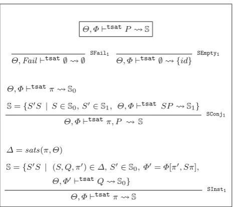
Fig. 4 Terminating constraint set satisfiability
Let f[x→y]denote the usual function updating notation for fgiven by f(x)=yifx=x, otherwise f(x).
We define [π0, π]as updating of (π0) = (I, ) as follows, whereI =(v0, v1, . . . , vn),π =Cτ1· · ·τn,n0= η(π):
[π0, π] = [π0→((n0, v1, . . . , vn), )]ifn0< I.v0; [π0→(I, ∪ {π})]ifn0= I.v0, π ∈; [π0→(I, )]if n0>I.v0,∃i. (I.vi = −1)
where, fori =1, . . . ,n, I.vi =
−1 ifI.vi < η(τi)ori=0
η(τi) otherwise Failotherwise
The computable function (tsat) for constraint satis-fiability, defined in Fig. 4, uses judgements of the form
, tsat P S, with constraint-head-value function as additional parameter.
The set of satisfying substitutions for constraint setPwith respect to the set of constraint axiomsis given byS, such that , 0 tsat P Sholds, where 0(π0) = (I0,∅) for each constraint headπ0 = Cτ1... τninandI0is a tuple formed byn+1 occurrences of a large enough integer constant, represented by∞.
Consider the following.
Example 3 Consider computing satisfiability ofπ=Eq[[I]] in= {EqI,∀a.Eq a⇒Eq[a]}, lettingπ0=Eq[a]; we have:
0=sats(π, )= {
S|∅,{Eq[I]}, π0
}
S= [a1→ [I]]
S0= {S1◦id| S1∈S1, , 1tsat Eq[I]S1}
where 1= 0[π0, π], 1(π0).I =(η(π)=3,∞),Sπ = πanda1is a fresh type variable; then:
1=sats(Eq[I], )= {
S|∅,{EqI}, π0
}
S= [a2→I]
S1= {S2◦id| S2∈S2, , 2tsat EqIS2} , 1tsat Eq[I]S1
where 2= 1[π0,Eq[I]]andη(Eq[I])=2 is less than 1(π0).I.v0=3; then:
2=sats(EqI, )= {
id,∅,EqI}
S2= {S3◦id| S3∈S3, , 3tsat∅S3= {id}}
, 2tsat EqIS2
where 3= 2[EqI,EqI],S3= {id}by (SEmpty1).
Example 4 Consider again Example2: we want to obtain the set of satisfying substitutions for constraintπ =C a(T a), given= {∀a,b.C a b⇒C(T2a)b}(computation with inputπ by the function in Fig. 3does not terminate). We have, whereπ0=C(T2a)b:
0=sats(π, )= {
S|{a},{π1}, π0
}
S = [a→T2a1,b1→T3a1] π1=C a1(T3a1)
S0= {S1◦ [a→T2a1] |S1∈S1, , 1tsatπ1S1}
, 0tsatπ S0
where 1= 0[π0,Sπ],η(Sπ)=η(C(T2a1) (T3a1))= 7< 0(π0).I.v0= ∞; then:
1=sats(π1, )= {
S|{a1}, {π2}, π0
}
S= [a1→T2a2,b2→T3a1=T5a2] π2=C a2(T5a2)
S1= {S2◦[a1→T2a2] |S2∈S2, , 2tsatπ2S2}
, 1tsatπ1S1
where 2 = 1[π0,Sπ1], Sπ1 = (C (T2 a2) (T5a2) and, sinceη(Sπ1)= 9 > 1(π0).I.v0 = 7, we have that
2(π0).I =(−1, η(T2a2)=3, η(T5a2)=6); then: 1=sats(π2, )= {
S|{a2}, {π3}, π0
}
S = [a2→T2a3,b3→T5a2=T7a3] π3=C a3(T7a3)
S2= {S3◦[a2→T2a3] |S3∈S3, , 3tsatπ3S3}
, 1tsatπ1S2
where 3 = 2[π0,Sπ2] = Fail, because η(Sπ2) = η(C(T3a3) (T7a3))=12> 2(π0).I.v0=9 and there’s noisuch that 3(π0).I.vi = −1, meaning that no parameter
ofSπ2has a decreasingηvalue.
The following illustrates an example of a satisfiable con-straint for which computation of satisfiability involves com-puting satisfiability of constraintsπthat unify with a con-straint headπ0such thatη(π)is greater than the upper bound associated toπ0.
Example 5 Consider satisfiability ofπ=CI(T3I)in=
{C(T a)I,∀a,b.C(T2a)b⇒C a(T b)}. We have, where
π0=C a(T b):
0=sats(π, )= {
S|∅,{π1}, π0
}
S= [a1→I,b1→T2I] π1=C(T2I) (T2I)
S0= {S1◦id|S1∈S1, , 1tsatπ1S1}
, 0tsatπ S0
where 1 = 0[π0, π],η(π) =5 < 0(π0).I.v0 = ∞,
Sπ =π; then:
1=sats(π1, )= {
S|∅,{π2}, π0
}
S= [a2→T2I,b2→TI]
π2=C(T4I) (TI)
S1= {S2◦ [a1→T2a2] |S2∈S2, , 2tsatπ2S2}
, 1tsatπ1S1
where 2 = 1[π0, π1], 1(π0).I =(5,∞,∞),Sπ1 = π1. Sinceη(π1) = 6 > 5 = 1(π0).I.v0, we have that
2(π0).I becomes equal to(−1,3,3).
Then, consider thatπ2=Cτ1τ2whereτ1=T4Iandτ2=
T I. Sinceη(π2) > 2(π0).I.v0= −1, there must existi, 1≤i ≤2, such thatη(τi) < 2(π0).vi, and such condition
is satisfied for i = 2, updating 2(π0).I to (−1,−1,2). Satisfiability is then finally tested forπ3 =C(T6I)I, that unifies with π0 = C(T a)I, which returnsS3 = {[a3 →
T5I]|
∅} = {id}. Constraintπ is thus satisfiable, withS0 = {id}.
The following example illustrates the use of a set of con-straints as a component of the constraint-head-value function.
Example 6 Let π = C(T2I)F, π0 = C(T a)b, = {CI(T2F),∀a,b.C a(T b)⇒C(T a)b}:
0=sats(π, )= {
S|∅,{π1}, π0
}
S= [a1→(TI),b1→F], π1=C(T I) (T F)
S0= {S1◦id| S1∈S1, , 1tsatπ1S1}
, 0tsatπS0
where 1= 0[π0, π],Sπ=π; then: 1=sats(π1, )= {
S|∅,{π2}, π0
}
S= [a2→I,b2→TF], π2=CI(T2F)
S1= {S2◦id| S2∈S2, , 2tsatπ2S2}
, 1tsatπ1S1
where 2 = 1[π0, π1],η(π1) = 4 = 1(π0).I.v0 = η(π), Sπ1 = π1 and π1 is not in 1(π0).1 = ∅. We have that S2 = {id}, because sats(CI(T2F), ) = {(id,∅,CI(T2F))}, andπis then satisfiable.
(PCP) instance by means of constraint set satisfiability, using G. Smith’s scheme [6], is shown below. For all examples mentioned in the literature [15,17] and numerous tests that include those used by GHC involving pertinent GHC exten-sions, the algorithm works as expected, without the need of any compilation flag.
Example 7 This example uses a PCP instance taken from [9]. A PCP instance can be defined as composed of pairs of strings, each pair having a top and a bottom string, where the goal is to select a sequence of pairs such that the two strings obtained by concatenating top and bottom strings in such pairs are identical. The example uses three pairs of strings:p1=(100,1)(that is, pair 1 has string100as the top string and1as the bottom string), p2 = (0,100)and
p3=(1,00).
This instance has a solution: using numbers to represent corresponding pairs (i.e.,1represents pair 1 and analogously for2and3), the sequence of pairs1311322is a solution.
A satisfiability problem that has a solution if and only if the PCP instance has a solution can be constructed by adapting G. Smith’s scheme to Haskell’s notation. We consider for this a two-parameter classC, and a constraint context such that
=1∪2∪3, whereiis constructed from pairi, for i =1,2,3:
1= {C(1→0→0)1,
∀a,b.C a b⇒C(1→0→0→a) (1→b)}
2= {C0(1→0→0),
∀a,b.C a b⇒C(0→a) (1→0→0→b)}
3= {C1(0→0),
∀a,b.C a b⇒C(1→a) (0→0→b)}
We have that constraintC a a is satisfiable, with a solution constructed from solution1311322of the PCP instance. Computation by our algorithm terminates, erroneously reporting unsatisfiability. The steps of the computation are omitted. The error occurs because a constraint π2 =
C a2(1 → a2)unifies with π01 = C(1 → 0 → 0 →
a) (1 → b)andη(Sπ2)is greater than (π01).I.v0, where
S = mgu(π2, π01), and there’s no i ∈ {1,2} such that 3(π0).I.vi = −1, meaning that no parameter ofSπ2has a decreasingηvalue.
To prove that the computation of the set of satisfying substitutions for any given constraint set P by the func-tion defined in Fig. 4 always terminates, consider that an infinite recursion might only occur if an infinite number of constraints unified with the headπ0of one constraint axiom in, since there exist finitely many constraint axioms in. This is avoided because, for any new constraintπthat unifies withπ0, we have, by the definition of [π0, π], that (π0) is updated to a value distinct from the previous ones (other-wise [π0, π]yieldsFailand computation is stopped). The conclusion follows from the fact that (π0)can have only
finitely many distinct values, for anyπ0. This can be seen by considering that, for anyπ0such that (π0)=(I, ), the insertion of a new constraint indecreasesk−k, wherekis the finite number of all possible values that can be inserted in
andkis the cardinality of. Such a decrease causes then a decrease of (since there exists only finitely many con-straint headsπ0in). Similarly, at each step there must exist somei such thatI.vi decreases, and this can happen only a
finitely number of times. We conclude that computation on any given input terminates.
The proposed termination criteria is related to thePaterson Conditionused in the GHC compiler (see Sect.2). The con-straint value is based on item 2 of this condition, but, instead of using it as a syntactic restriction over constraint heads and contexts in instance declarations, we use it in the defini-tion of a finitely decreasing chain over recursively dependent constraints.
In comparison to the use of a recursion depth limit, our approach has the advantage that type-correctness is not implementation dependent (a constraint is or is not satisfiable with respect to a given set of constraint axioms). The use of a recursion depth limit can make a constraint set satisfiable in one implementation and unsatisfiable in another that uses a lower limit. Incorrectly reporting unsatisfiability can occur in both cases, but is expected to be extremely rare with our approach. We are not aware of any practical example where this occurs.
The main disadvantages of our approach are that it is not syntactically possible to characterize such incorrect unsat-isfiability cases and it is not very easy for programmers to understand how type class constraints are handled in such a case, if and when it occurs. However, we expect these cases not to occur in practice.
The presented algorithm has been verified to behave cor-rectly, without the need of any compilation flag, on all exam-ples found in the literature [15], all GHC test cases, involving flagsFlexibleInstances,FlexibleContextsand UndecidableInstances, and on Haskell libraries that use multi-parameter type classes, including the monad trans-former library [1].
5 Constraint set simplification
The process of simplification of a constraint set, also called context reduction, consists of reducing each constraintπ in this set to the context obtained by recursively reducing the contextPof thematching instanceforπin, if such match-ing exists, until P = ∅or there exists no instance inthat matches withπ. In the latter caseπreduces to itself.
This recursive process may not terminate: as a simple example, consider reduction of constraint C a when =
This section presents a computable function for constraint set simplification, where computation is guaranteed to termi-nate by using the same criterion used in Sect.4.1.
Constraint set simplification is essentially based on instance matching. We use functionmatches(π, ), defined below, in order to capture the relevant information of match-ing constraint axioms inwith a given constraintπ. Func-tion matches is defined by using function sats (Sect. 4), through skolemization of type variables that occur in the given constraint argument (Skolem variables are non unifi-able variunifi-ables, that is, constants):
matches(π, )=
(S P, π)|=sats[α→K]π, ,
(S,S P, π)∈, α=tv(π), K are fresh Skolem variables
Function matches(π, ) returns either a singleton or an empty set2.
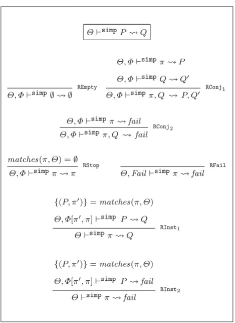
Constraint set simplification uses a function defined in Fig.5by means of judgements of the form, simp
P Q. This means that reduction of constraint setPunder con-straint axiomseither give constraint set Q as a result or fails. Failure is caused by the criterion used for ensuring ter-mination, explained in Sect.4.1. Using this function, context reduction is defined as follows, where 0 is as defined in Sect.4.1:
fori =1, . . . ,n, Qi =
πi if, 0simpπi fail Qi if, 0simpπi Qi
simp0 {π
1, . . . πn} Q1, . . . ,Qn
R0
The rules of Fig.5are analogous to the ones in Fig. 4, but now termination enforced by the termination criterion is reported as a failure, which must be propagated back-wards along the recursive calls of the computation. Thus, reduction of a constraint π is now defined by two rules, (RInst1) and (RInst2) and, analogously, two different rules are used for specifying reduction of a non-singleton set of constraints.
Rule (REmpty) specifies that an empty set of constraints reduces to itself. Rule (RStop) specifies that a constraintπ cannot be reduced if there is no instance inthat matches withπ. Rule (RFail) enforces termination, expressing that reduction cannot be performed since updating of fails.
The process of constraint set simplification is illustrated by the following example.
2We do not consideroverlapping instances[20], since the subject is
unrelated to termination of constraint set satisfiability and simplifica-tion. Supporting overlapping instances would need a modification of functionmatchesso as to select a single instance if there exist overlap-ping matching instances.
Fig. 5 Constraint set simplification
Example 8 Let = {∀a.C(T a)⇒ C a, DI}and P =
{DI,C a}. According to rule (R0)reduction of P amounts to independently reducing constraintsDIandC a.
Reduction ofDIis defined by rule (RInst1): {(∅,DI)} =matches(DI, )
, 0[DI,DI] simp∅∅
, 0simp DI∅
Reduction of π = π0 = C a results in failure, as shown below:
{(C(T a1), π0)} =matches(π, ) , 1simp(C(T a1))fail
, 0simpπfail
where 1 = 0[π, π0], 1(π0).I = (η(π) = 1,∞). We have that:
{(C(T2a2), π0)} =matches(C(T a1), ) , 2simp(C(T2a2))fail
, 1simp(C(T a1))fail
where 2= 1[C(T a1), π0] = failbecauseη(C(T a1)) < 1(π0).I.v1=1.
The following theorem states the correctness of the con-straint simplification function defined in Fig.5.
Theorem 3 [Correctness ofsimp
]If, simp
P Q holds, then,Q P is provable and Q cannot be further simplified, i.e., , simp
QQ.
Proof Induction over, simp P Q.
6 Conclusion
This paper presents a termination criterion and terminating algorithms for constraint simplification and improvement, based on the use of a value that always decreases on each recursive step in these algorithms. The termination criterion defined can be used in any form of constraint simplification and improvement algorithm during type inference.
The use of this criterion eliminates the need for imposing syntactic conditions on Haskell type class and instance decla-rations and the need for using a recursion stack depth limit in order to guarantee termination of type inference in the pres-ence of multi-parameter type classes, in case these syntactic conditions are chosen by programmers not to be enforced.
Since type class constraint satisfiability is in general unde-cidable, there exist instances of this problem for which the algorithm presented in this paper incorrectly reports unsatis-fiability. However, practical examples where this occurs are expected to be very rare. The algorithms have been imple-mented and used in a prototype front-end for Haskell, avail-able athttp://github.com/rodrigogribeiro/mptc. For all exam-ples mentioned in the literature, Haskell libraries that use multi-parameter type classes and tests used by the Haskell GHC compiler, involving all pertinent GHC extensions, the algorithm works as expected without the need for any com-pilation flag.
In comparison to the use of a recursion depth limit, our approach has the advantage that type-correctness is not implementation dependent (a constraint is or is not satisfiable with respect to a given set of constraint axioms). The use of a recursion depth limit can make a constraint set satisfiable in one implementation and unsatisfiable in another that uses a lower limit. Incorrectly reporting unsatisfiability can occur in both cases, but is expected to be extremely rare with our approach. We are not aware of any practical example where this occurs.
The main disadvantages of our approach are that it is not syntactically possible to characterize such incorrect unsat-isfiability cases and it is not very easy for programmers to understand how type class constraints are handled in such a case, if and when it occurs.
Acknowledgments We would like to thank the anonymous review-ers for their careful work, which has been very useful to improve the paper.
References
1. Gill A (2006) MTL–The Monad Transformer Library. http:// hackage.haskell.org/package/mtl
2. Baader F, Snyder W (2001) Unification theory. In: Robinson J., Voronkov A (eds) Handbook of Automated Reasoning, Elsevier Science Publishers, vol. 1, pp 447–533
3. Camarão C, Figueiredo L, Vasconcellos C (2004) Constraint-set Satisfiability for Overloading. In: Proc. of the 6th ACM SIGPLAN International Conf. on Principles and Practice of Declarative Pro-gramming (PPDP’04), pp 67–77
4. Camarão C, Ribeiro R, Figueiredo L, Vasconcellos C (2009) A Solution to Haskell’s Multi-Parameter Type Class Dilemma. In: Proc. of the 13th Brazilian Symposium on Programming Lan-guages (SBLP’2009), pp 5–18.http://www.dcc.ufmg.br/camarao/ CT/solution-to-mptc-dilemma.pdf
5. Hall C, Hammond K, Jones SP, Wadler P (1996) Type Classes in Haskell. ACM Trans Program Lang Syst 18(2):109–138 6. Smith G (1991) Polymorphic type inference for languages with
overloading and subtyping. Ph.D. thesis, Cornell Univ.
7. Jones M, Diatchki I (2008) Language and Program Design for Functional Dependencies. In: ACM SIGPLAN Haskell, Workshop, pp 87–98
8. Jones SP et al. (2003) The Haskell 98 Language and Libraries: The Revised Report. J Func Prog 13(1):0–255.http://www.haskell.org/ definition/
9. Zhao L (2002) Solving and Creating Difficult Instances of Posts Correspondence Problem. Department of Computer Science, University of Alberta, Master’s thesis
10. Chakravarty M, Keller G, Jones SP (2005) Associated type syn-onyms. In: Proc. of the 10th ACM SIGPLAN International Conf. on Functional Programming (ICFP’05), pp 241–253
11. Chakravarty M, Keller G, Jones SP, Marlow S (2005) Associated types withclass.In: Proc. of the ACM Symp. on Principles of Prog. Languages (POPL’05), pp 1–13
12. Jones M (1994) Qualified Types. Cambridge University Press, Cambridge
13. Jones M (1995) Simplifying and Improving Qualified Types. In: Proc. of the ACM Conf. on Functional Prog. and Comp. Archi-tecture (FPCA’95), pp 160–169
14. Jones M (2000) Type Classes with Functional Dependencies. In: Proc. of the European Symp. on Programming (ESOP’2000). LNCS 1782
15. Sulzmann M, Duck G, Jones SP, Stuckey P (2007) Understand-ing functional dependencies via constraint handlUnderstand-ing rules. J Funct Program 17(1):83–129
16. Milner R (1978) A theory of type polymorphism in programming. J Comput Syst Sci 17:348–375
17. Stuckey P, Sulzmann M (2005) A Theory of Overloading. ACM Trans Prog Lang Syst (TOPLAS) 27(6):1216–1269
18. Wadler P, Blott S (1989) How to make ad-hoc polymorphism less ad-hoc. In: Proc. of the 16th ACM Symp. on Principles of Prog. Lang. (POPL’89), pp 60–76. ACM Press, New York
19. Jones SP et al (1998) GHC–The Glasgow Haskell Compiler.http:// www.haskell.org/ghc/