Feedback policy rules for government
spending: an algorithmic approach
Ilias Kostarakos
*and Stelios Kotsios
1 Background
One of the most important objectives of economic policy is to ensure, via the appro-priate manipulation of the available policy instruments (control variables), that the economic system tracks, as closely as possible, a desired path for the policy targets (out-puts). One of the approaches that has been utilized for the design of economic policy is the feedback approach, stemming from the mathematical control theory literature. Vari-ous aspects of the feedback methodology have been utilized for the purposes of policy design for more than 50 years, starting with the use of PID controllers in the seminal paper by Phillips (1954). These aspects range from (stochastic) optimal feedback con-trol (see, among others, Amman and Kendrick 2003; Christodoulakis and Levine 1987; Christodoulakis and Van Der Ploeg 1987; Leventides and Kollias 2014) to nonlinear (Athanasiou et al. 2008; Athanasiou and Kotsios 2008; Kotsios and Leventidis 2004) and stochastic control applications (Dassios et al. 2014).
The importance of feedback rules for policy design is evident from the fact that for more than 20 years monetary policy decisions have been, to a large extent, based on the Taylor rule (see Taylor 1993); this is a linear feedback policy rule stipulating (in its simplest form) that the interest rate is set based on deviations of inflation and GDP from target levels of inflation and potential GDP, respectively. It is interesting to note here that Taylor presented a rule that had fixed settings for the parameters; in particular:
(1) r=p+0.5y+0.5(p−2)+2
Abstract
We present an algorithmic approach for the design of fiscal policy rules. In particu-lar, using algorithmic feedback control techniques, we design linear feedback policy rules such that predetermined target levels for GDP and public debt are simultane-ously, exactly tracked. We run a number of simulations in order to examine the effects of different policy response rates and the overall effectiveness of the proposed methodology.
Keywords: Fiscal policy, Public debt, Linear feedback control, Algorithmic control
Open Access
© The Author(s) 2017. This article is distributed under the terms of the Creative Commons Attribution 4.0 International License (http://creativecommons.org/licenses/by/4.0/), which permits unrestricted use, distribution, and reproduction in any medium, provided you give appropriate credit to the original author(s) and the source, provide a link to the Creative Commons license, and indicate if changes were made.
RESEARCH
where r is the federal funds rate, p the rate of inflation and y the percentage deviation of real GDP from a target (e.g., potential output). The rule stipulates that, for example, if GDP exceeds its full-employment level, then nominal interest rates need to be increased.
One of the advantages of adopting the feedback framework is that it allows to explic-itly take into account the time lags associated with the conduct of economic policy, since they can be incorporated into the dynamics of the model and the feedback policy rule (Kendrick 1988). Most importantly, the feedback methodology allows for more frequent (and, possibly, smaller) interventions by the policymaker, which are likely to result in a
smoother transition path for the economy (see Kendrick and Amman 2014; Kendrick
and Shoukry 2014).
Our aim in this paper is to utilize the algorithmic feedback control framework for the design of short-term fiscal policy interventions. That is, we want to design linear feed-back policy rules for the fiscal policy instruments available so that predetermined (fixed) desired sequences for the policy targets (GDP and public debt levels) are simultaneously tracked. In particular, we assume that the policymaker has at his disposal two instru-ments: expenditures related to compensation of public sector employees, social benefits, etc. (i.e., expenditures that cover individual and collective consumption) and expendi-tures related to investment projects (e.g., infrastructure) that will be funded by the gov-ernment (either via its own budget or by using external funding such as EU structural funds or the funds available from the so-called Juncker Investment Plan). These invest-ment expenditures are subject to several time lags (including, among others, legislative, design and implementation lags), and as a result, they will affect the economy with a possibly substantial delay; however, the feedback mechanism used allows us to explicitly incorporate these lags into the design of the fiscal policy rules. These rules will provide the exact sequence of the policy instruments necessary to ensure that the target levels of GDP and public debt will be simultaneously met, without any deviation (thus, the track-ing error will be equal to zero).
In order to design the policy rules, we use an algorithmic linear feedback control technique known as (exact) model matching control. It is a completely parameterized technique allowing us to develop appropriate symbolic algorithms in order to design the requested policy rules. One of the main advantages of this approach is that we obtain as a solution a class of feedback policy rules; this grants the policymaker the ability to choose the most appropriate policy rule from the set of potential policies available, depending on the particular case at hand. Moreover, the policy rules take into account the state of the economy, since they incorporate the relevant information available up to the decision period, and they are responsive (i.e., the coefficients of the algebraic expres-sions are not fixed), thus representing a more discretionary approach to the design of fiscal policy.
Our analysis is conducted in the context of a linear, deterministic variant of the stand-ard multiplier–accelerator model proposed by Samuelson (1939). The main reason for choosing this simple linear model is its tractability, as it will allow us to thoroughly examine the effects of the proposed methodology on the workings of the system.
2 Formulation of the model
As already stated in the introduction, the model we chose is a linear, deterministic vari-ant of the multiplier–accelerator model coupled with the government budget constraint. This model has been extensively used in the relevant literature, due to its tractability and because it can easily be extended to both nonlinear and stochastic variants (see, among others, Dassios and Zimbidis 2014; Dassios and Devine 2016; Dalla and Varelas 2016; Dalla et al. 2016; Hommes 1995; Puu 2007).
The multiplier–accelerator part of the model consists of an income identity and four behavioral equations. Assuming a closed economy, the income identity is given by:
where t ∊ N is the time index and the real sequences C(t), I(t), Gw(t) and GI(t) denote consumption, private investment, general government expenditures (compensation of employees, social benefits, etc.) and government investment, respectively. For the λi parameters, we assume that λi ∊ (0, 1) and λ0 + λ1 + λ2 = 1. As already stated, govern-ment investgovern-ment-related expenditures are subject to various time lags, such as legislative (e.g., the time until the projects to be funded by the government are approved by the relevant parliamentary committee) and implementation lags (the time until the funds are actually disbursed) and, as a result, the policy will hit the economy with a (possibly substantial) delay and its effects will become apparent in subsequent periods.
These lags are captured by the λi parameters, which indicate the percentage of the gov-ernment’s decision to invest in period t that is realized in period t + i; that is, the λi parameters represent the percentage of the funds that the government aims to invest in period t that are actually disbursed in period t + i.
Moving on to the behavioral equations, the consumption function following Puu (2007) is given by:
where s ∊ (0, 1) is the marginal propensity to save and
is the disposable income. For the tax function, we assume that it takes the following tax-on-income form:
where τ ∈(0, 1) is the constant tax rate.
Investment depends on the accelerator principle:
where v > 1 denotes the accelerator.
Finally, the government budget constraint has the standard form:
(2) Y(t)=C(t)+I(t)+0GI(t)+1GI(t−1)
+ 2GI(t−2)+Gw(t)
(3) C(t)=(1−s)Yd(t−1)+sYd(t−2)
(4) Yd(t)=Y(t)−T(t)
(5) T(t)=τY(t)
(6) I(t)=v(Y(t−1)−Y(t−2))
where B(t) denotes debt outstanding and r is the (constant) interest on public debt. After all the necessary substitutions among Eqs. (2)–(7) and some necessary algebra, we end up with the following pair of equations:
where a1=(1−s)(1−τ )+v,a2=s(1−τ )−v. This is the input–output form of the model, with Y(t), B(t) being the outputs (policy targets) and GI, Gw being the inputs (pol-icy instruments).
3 Solution technique
Our aim is to design linear feedback policy rules for short-term fiscal policy interven-tions (that is, for the next 4–6 quarters). In particular, we want to design policy rules for general government expenditure (Gw(t)) and government investment (GI(t)) which, once implemented, will modify the dynamics of the system in such a way that predetermined, desired sequences for the levels of GDP and public debt will be simultaneously, exactly tracked.
The feedback rules relate the current value of the policy instruments to lagged values of both the instruments and the targets; thus, the requested linear feedback policy rules will be functions of the form:
where ai,cj,. . .,ns are unknown, real parameters to be determined. The solution method
provides us with a class of policy rules (that is, different specifications for the algebraic expressions) which ensures that the policy rules are responsive (see Taylor 1993). This is in contrast to rules that specify fixed settings for the instruments (e.g., the k% rule for money supply growth proposed by Friedman), and thus, these rules represent a more discretionary approach to the design and exercise of fiscal policy. Moreover, the dependence of the current values of the instruments on lagged values of both the instru-ments and the targets is a fundamental property of feedback rules known as causality
(see Astrom and Wittenmark 1996), essentially ensuring that the policy rules take into account all the relevant information available regarding the state of the economy.
In order to design the feedback policy rules, we use a technique from the control theory literature known as (exact) model matching; it is a completely parameterized technique, allowing for proper symbolic algorithms to be developed. In what follows, we provide a brief description of the workings of the model matching approach (see (8)
Y(t)−a1Y(t−1)−a2Y(t−2)
=0GI(t)+1GI(t−1)
+2GI(t−1+Gw(t)B(t) −(1+r)B(t−1)+τY(t)
=GI(t)+Gw(t)
(9) GI(t)=aiGI(t−i)+cjGw
t−j
+dhY(t−h)+
efB
t−f
Gw(t)=kpGI(t−p)+lqGw(t−q)
+mrY(t−r)+
“Appendix 1” for the mathematical formulation and the paper by Kostarakos and Kotsios 2017; Kotsios and Kostarakos 2016 for the relevant theorems and proofs): We want to design linear policy rules of form (9) which will modify the dynamics of original system (8)—the open-loop system—in such a way that predetermined, fixed targets for both out-puts are simultaneously reached. We work as follows: First, the policymaker decides on the desired vector sequence for the policy targets, say
Then, using an appropriate symbolic algorithm we construct a linear (artificial) system, which has the property that its output is identical to the desired sequence x�∗(t); this is
known as the desired system. Now, the problem at hand reduces to that of calculating the unknown parameters of policy rules (9) such that the original system becomes iden-tical, i.e., it is matched to the desired one. Again, the parameters are calculated using an appropriate symbolic algorithm (see Kostarakos and Kotsios 2017; Kotsios and Kostara-kos 2016; Kotsios and Leventidis 2004 for a detailed analysis of both algorithms).
The most important advantage of this approach is that the algorithms provide as a solution a class of feedback policy rules (that is, the coefficients of the algebraic expres-sions of the resulting policy rules are not fixed), which essentially constitutes a set of potential policies. Thus, the policymaker is able to choose from this set those rules he deems more appropriate, depending on the problem at hand. This grants the policy-maker the ability to take into account further considerations, such as the possible costs incurred from the implementation of the proposed policy plan and rule out politically infeasible rules. This class of policy rules can be augmented by calculating more complex rules (e.g., rules that contain more lags for the instruments and the targets). Another important advantage is that we can calculate the exact sequence of the policy instru-ments necessary for tracking the desired target levels; that is, the sequence necessary for reaching the targets without any deviations. Moreover, the rules are such that the system immediately settles on the desired path: If the rule is applied in period t, then the system starts following the desired trajectory from t + 1. Therefore, these policy rules are
“opti-mal,” in the sense that they ensure zero settling time to the desired path. Finally, we can simulate the model under different policy rules in order to obtain a better insight as to how the policy rules affect the working of the system, under different specifications and policy scenarios.
4 An application
From an economic policy point of view, the timing of the policy action is a central issue. In particular, given the lags associated with policy conduct, should the govern-ment immediately react to signs of a downturn in economic activity via, for example, a frontloaded disbursement of investment funds or would it be preferable to adopt a more gradual response? Moreover, how do the lags associated with policy conduct affect the actual implementation of the policy and its effects? In the analysis presented in Sect. 2, we saw that the policy lags are incorporated into our model via the λi parameters, using the following mechanism:
�
x∗(t)=
Y∗(t),B∗(t)T.
Then, for the cases where λ2 > λ0, the government manages to immediately react to signs of a crisis (since a bigger percentage of the expenditures will be disbursed in period t), while for λ0 > λ2, the bulk of the investment expenditures will actually be disbursed in period t + 2; this implies that the changes in the size of government investment will have
an effect in the economy with a two-period delay.
In order to examine the effects of different policy response times, we conducted a series of simulations. In particular, we examine the following cases for the λi, parameters:
1. The immediate response case: 0=0.2, 1=0.2, 2=0.6 2. The gradual response case: 0=0.4, 1=0.3, 2=0.3
3. The delayed response case: 0=0.5, 1=0.25, 2=0.25
We assume the following plausible values for the rest of the parameters of open-loop system (8):
Then, the open-loop system is:
Finally, the initial conditions are given in Table 1 and they depict an economy facing a severe downturn, with large decreases in GDP levels, accompanied with large increases in debt levels. Moreover, government investment-related expenditures GI have exhibited a large decline (possibly as a result of the policymaker’s efforts to reduce the budget).
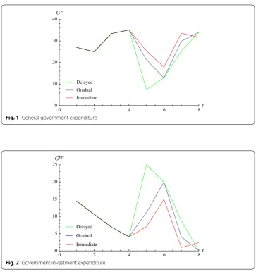
We assume that the government aims for a 1% per period increase in GDP levels and a corresponding decrease in the levels of debt. Figures 1 and 2 present the time paths of the control variables under all policy scenarios (a table with the results can be found in “Appendix 2”).
The results of the numerical simulations are summarized in the following theorem:
Theorem 1 The numerical simulations indicate that the faster the response of the government in the face of a downturn, the smaller the necessary changes in the compo-sition of government expenditure. On the contrary, if the response of the government is delayed, then large and abrupt changes are required rendering the policy plans politically infeasible.
v=1, s=0.2, τ =0.4, r=0.04
Y(t)−1.54Y(t−1)+0.94Y(t−2)=0GI(t)
+1GI(t−1)+2GI(t−2)+Gw(t)
B(t)−1.04B(t−1)+0.4Y(t)=GI(t)+Gw(t)
Table 1 Initial conditions
Time Y B GI Gw
1 120 135 14.45 27
2 112 142 10.63 25
3 105 145 6.9 33.42
As we can clearly see in the figures, the response time is critical regarding the compo-sition of total government expenditures, i.e., the allocation between investment-related expenditures (GI(t)) and general government expenditures (Gw(t)) as well as regarding the necessary changes in the size of the policy instruments. In particular, when the gov-ernment is able to immediately respond to a downturn (λ2 > λ0 case), then GI(t) needs to slightly increase in the first two periods of policy implementation, in order to provide a boost to the economy via the multiplier principle. At the same time, Gw(t) needs to be cumulatively decreased by 10%, to ensure that a surplus is generated so that a reduction in debt levels can be achieved. On the contrary, when the response time entails consid-erable lags λ0 > λ2 case, the size of the changes of the policy instruments is significantly larger. Government investment funds need to be immediately increased due to the fact that this change will only hit the economy after two periods, and they exhibit a cumula-tive increase of 48.8%. As a result of these increases, Gw(t) exhibits a sharp decline over the entire period (almost a 34% reduction), in order to achieve the debt reduction target. Such abrupt and large changes in the composition of total government expenditures are most likely politically infeasible. In the gradual response case, the necessary changes are
0 2 4 6 8t
0 10 20 30 40
Gw
Delayed Gradual Immediate
Fig. 1 General government expenditure
0 2 4 6 8t
0 5 10 15 20 25
GInv
Delayed Gradual Immediate
smaller and both instruments exhibit smooth transition paths. The results highlight the need for fast action by the policymaker, combined with frequent interventions (which is made possible when the feedback framework for policy design is adopted).
5 Conclusions
In this paper, we presented an application of algorithmic linear feedback control for the design of short-term fiscal policy. In particular, in the context of a linear deterministic variant of the multiplier–accelerator model, using an algebraic control theory technique known as exact model matching, we designed a class of linear feedback laws such that the system will immediately track a predetermined, desired trajectory for both policy targets, without any deviations. Moreover, in order to examine the effects of time lags, we run some simulations under different policy response rates. An important implica-tion of the policy experiments is that immediate response allows the government to achieve the policy targets with relatively small policy interventions, compared to cases where there are larger delays in the disbursement of funds.
Authors’ contributions
The authors wish to declare that the article was written in collaboration—each author contributed to 50% of the article. Both authors read and approved the final manuscript.
Competing interests
The authors declare that they have no competing interests.
Appendix 1: Mathematical formulation of the model matching problem
In this appendix, we provide the basic mathematical formulation of the model matching technique, elaborated in Sect. 3.
First, we have to rewrite input–output model (8) in a more compact form. This is done via using the notion of the q-operator, a lag operator defined as qif(t) = f(t − i), for any sequence f(t) (see Astrom and Wittenmark 1996). Then, system (8) can be written in the so-called algebraic form:
where �x(t)=(Y(t),B(t))T,u�(t)=(GI(t),Gw(t))T and
This is also known as the open-loop system, i.e., the system before the policy interven-tion. The desired system, that is the system having the property that its output is exactly equal to the desired sequence �x∗
(t), is of the form:
where Ad,Kd are 2 × 2 polynomial matrices constructed using an appropriate symbolic
algorithm.
Then, we want to calculate feedback policy rules which, once applied to open-loop sys-tem (8), will modify its dynamics in such a way that it will be identical, i.e., matched, to desired system (11). Feedback rules (9) can be written, using the q-operator, as:
A(q)�x(t)=K(q)u�(t)
(10) A=
1−a1q−a2q2 0 τ 1−(1+r)q
, K =
0+1q+2q2 1
1 1
(11) Ad(q)x�∗(t)=Kd(q)−→uc(t)
where R(q), S(q) and T(q) are unknown polynomial matrices in q to be designed. It turns out that if the following set of equations holds:
then policy rules (12) can ensure that open-loop system (10) will be matched to the desired one.
These equations are solved using appropriate symbolic algorithms developed in Math-ematica (see Kotsios and Kostarakos 2016).
Appendix 2: Table of results
The following table presents the time paths of the policy instruments under all the time-response cases (Table 2).
Received: 31 October 2016 Accepted: 24 February 2017
References
Amman H, Kendrick D (2003) Mitigation of the Lucas critique with stochastic control methods. J Econ Dyn Control 27:2035–2057
Astrom K, Wittenmark B (1996) Computer-controlled systems: theory and design, 3rd edn. Prentice Hall, Prentice Athanasiou G, Kotsios S (2008) An algorithmic approach to exchange rate stabilisation. Econ Model 25:1246–1260 Athanasiou G, Karafyllis I, Kotsios S (2008) Price stabilization using buffer stocks. J Econ Dyn Control 32:1212–1235 Christodoulakis N, Levine P (1987) The trade-off between simplicity and optimality in macroeconomic policy design. J
Econ Dyn Control 11:173–178
Christodoulakis N, Van Der Ploeg F (1987) Macrodynamic formulation with connecting views of the economy: a synthesis of optimal control and feedback design. Int J Syst Sci 18:449–479
Dalla E, Varelas E (2016) Second-order accelerator of investment: the case of discrete time. Intern Rev Econ Educ 21:48–60 Dalla E, Karpetis C, Varelas E (2016) Modeling investment cycles: a theoretical analysis. Mod Econ 7:336–344
Dassios I, Devine M (2016) A macroeconomic mathematical model for the national income of a union of countries with interaction and trade. J Econ Struct 5:1–15
Dassios I, Zimbidis A (2014) The classical Samuelson’s model in a multi-country context under a delayed framework with interaction. Dyn Contin Discrete Impuls Syst Ser B Appl Algorithms 21:261–274
Dassios I, Zimbidis A, Kontzalis C (2014) The delay effect in a stochastic multiplier–accelerator model. J Econ Struct 3:7 Hommes C (1995) A reconsideration of hicks’ nonlinear trade cycle model. Struct Change Econ Dyn 6:4
Kendrick D (1988) Feedback: a new framework for macroeconomic policy, 1st edn. Springer, Netherlands Kendrick D, Amman H (2014) Quarterly fiscal policy. Econ Voice 11:7–12
Kendrick D, Shoukry G (2014) Quarterly fiscal policy experiments with a multiplier–accelerator model. Comput Econ 44:269–293
R(q)A(q)+K(q)S(q)=Ad(q)
K(q)T(q)=Kd(q)
R(q)K(q)=K(q)R(q)
Table 2 GI, Gw values for r = 4%
Time Immediate Gradual Delayed
GI Gw GI Gw GI Gw
5 7.023 25.37 11.138 21.26 24.998 7.4
6 14.954 17.91 19.991 12.88 19.981 12.89
7 0.388 33.57 4.065 29.89 8.689 25.27
8 2.39 31.72 0.121 33.99 0.047 34.06
Kostarakos I, Kotsios S (2017) Fiscal policy design in Greece in the aftermath of the crisis: an algorithmic approach. Com-put Econ. doi:10.1007/s10614-017-9650-3
Kotsios S, Kostarakos I (2016) Controlling national income and public debt via _fiscal policy. a model matching algorith-mic approach. Vestnik of Saint-Petersburg University. Series 10. Applied Mathematics. Computer Science. Control Processes (forthcoming)
Kotsios S, Leventidis J (2004) A feedback policy for a modified Samuelson–Hicks model. Int J Syst Sci 35:331–341 Leventides J, Kollias I (2014) Optimal control indicators for the assessment of the influence of government policy to
busi-ness cycle shocks. J Dyn Games 1:79–104
Phillips A (1954) Stabilisation policy in a closed economy. Econ J 64:290–323
Puu T (2007) The Hicksian trade cycle with floor and ceiling dependent on capital stock. J Econ Dyn Control 31:575–592 Samuelson P (1939) Interactions between the multiplier analysis and the principle of acceleration. Rev Econ Stat
21:75–78