A survey on Image Data Augmentation for Deep Learning

Introduction

Deep Learning models have made incredible progress in discriminative tasks. This has been fueled by the advancement of deep network architectures, powerful computation, and access to big data. Deep neural networks have been successfully applied to Com-puter Vision tasks such as image classification, object detection, and image segmenta-tion thanks to the development of convolusegmenta-tional neural networks (CNNs). These neural networks utilize parameterized, sparsely connected kernels which preserve the spatial characteristics of images. Convolutional layers sequentially downsample the spatial resolution of images while expanding the depth of their feature maps. This series of convolutional transformations can create much lower-dimensional and more useful rep-resentations of images than what could possibly be hand-crafted. The success of CNNs has spiked interest and optimism in applying Deep Learning to Computer Vision tasks.

Abstract

Deep convolutional neural networks have performed remarkably well on many Computer Vision tasks. However, these networks are heavily reliant on big data to avoid overfitting. Overfitting refers to the phenomenon when a network learns a function with very high variance such as to perfectly model the training data. Unfor-tunately, many application domains do not have access to big data, such as medical image analysis. This survey focuses on Data Augmentation, a data-space solution to the problem of limited data. Data Augmentation encompasses a suite of techniques that enhance the size and quality of training datasets such that better Deep Learning models can be built using them. The image augmentation algorithms discussed in this survey include geometric transformations, color space augmentations, kernel filters, mixing images, random erasing, feature space augmentation, adversarial training, generative adversarial networks, neural style transfer, and meta-learning. The applica-tion of augmentaapplica-tion methods based on GANs are heavily covered in this survey. In addition to augmentation techniques, this paper will briefly discuss other character-istics of Data Augmentation such as test-time augmentation, resolution impact, final dataset size, and curriculum learning. This survey will present existing methods for Data Augmentation, promising developments, and meta-level decisions for implementing Data Augmentation. Readers will understand how Data Augmentation can improve the performance of their models and expand limited datasets to take advantage of the capabilities of big data.

Keywords: Data Augmentation, Big data, Image data, Deep Learning, GANs

© The Author(s) 2019. This article is distributed under the terms of the Creative Commons Attribution 4.0 International License (http://creat iveco mmons .org/licen ses/by/4.0/), which permits unrestricted use, distribution, and reproduction in any medium, provided you give appropriate credit to the original author(s) and the source, provide a link to the Creative Commons license, and indicate if changes were made.

There are many branches of study that hope to improve current benchmarks by apply-ing deep convolutional networks to Computer Vision tasks. Improvapply-ing the generaliza-tion ability of these models is one of the most difficult challenges. Generalizability refers to the performance difference of a model when evaluated on previously seen data (train-ing data) versus data it has never seen before (test(train-ing data). Models with poor general-izability have overfitted the training data. One way to discover overfitting is to plot the training and validation accuracy at each epoch during training. The graph below depicts what overfitting might look like when visualizing these accuracies over training epochs (Fig. 1).

To build useful Deep Learning models, the validation error must continue to decrease with the training error. Data Augmentation is a very powerful method of achieving this. The augmented data will represent a more comprehensive set of possible data points, thus minimizing the distance between the training and validation set, as well as any future testing sets.

Data Augmentation, the focus of this survey, is not the only technique that has been developed to reduce overfitting. The following few paragraphs will introduce other solu-tions available to avoid overfitting in Deep Learning models. This listing is intended to give readers a broader understanding of the context of Data Augmentation.

Many other strategies for increasing generalization performance focus on the model’s architecture itself. This has led to a sequence of progressively more complex architec-tures from AlexNet [1] to VGG-16 [2], ResNet [3], Inception-V3 [4], and DenseNet [5]. Functional solutions such as dropout regularization, batch normalization, transfer learn-ing, and pretraining have been developed to try to extend Deep Learning for application on smaller datasets. A brief description of these overfitting solutions is provided below. A complete survey of regularization methods in Deep Learning has been compiled by Kukacka et al. [6]. Knowledge of these overfitting solutions will inform readers about other existing tools, thus framing the high-level context of Data Augmentation and Deep Learning.

Transfer Learning works by training a network on a big dataset such as ImageNet [12] and then using those weights as the initial weights in a new classification task. Typically, just the weights in convolutional layers are copied, rather than the entire network including fully-connected layers. This is very effective since many image datasets share low-level spatial characteristics that are better learned with big data. Understanding the relationship between transferred data domains is an ongoing research task [13]. Yosinski et al. [14] find that transferability is negatively affected primarily by the specialization of higher layer neurons and difficulties with splitting co-adapted neurons.

• Pretraining [15] is conceptually very similar to transfer learning. In Pretraining, the network architecture is defined and then trained on a big dataset such as ImageNet [12]. This differs from Transfer Learning because in Transfer Learning, the network architecture such as VGG-16 [2] or ResNet [3] must be transferred as well as the weights. Pretraining enables the initialization of weights using big datasets, while still enabling flexibility in network architecture design.

• One-shot and Zero-shot learning [16, 17] algorithms represent another paradigm for building models with extremely limited data. One-shot learning is commonly used in facial recognition applications [18]. An approach to one-shot learning is the use of siamese networks [19] that learn a distance function such that image classification is possible even if the network has only been trained on one or a few instances. Another very popular approach to one-shot learning is the use of memory-augmented net-works [20]. Zero-shot learning is a more extreme paradigm in which a network uses input and output vector embeddings such as Word2Vec [21] or GloVe [22] to classify images based on descriptive attributes.

test-time augmentation, curriculum learning, and the impact of resolution are covered in this survey under the “Design considerations for image Data Augmentation” section. Descriptions of individual augmentation techniques will be enumerated in the “Image Data Augmentation techniques” section. A quick taxonomy of the Data Augmentations is depicted below in Fig. 2.

Before discussing image augmentation techniques, it is useful to frame the context of the problem and consider what makes image recognition such a difficult task in the first place. In classic discriminative examples such as cat versus dog, the image recognition software must overcome issues of viewpoint, lighting, occlusion, background, scale, and more. The task of Data Augmentation is to bake these translational invariances into the dataset such that the resulting models will perform well despite these challenges.

It is a generally accepted notion that bigger datasets result in better Deep Learning models [23, 24]. However, assembling enormous datasets can be a very daunting task due to the manual effort of collecting and labeling data. Limited datasets is an especially prevalent challenge in medical image analysis. Given big data, deep convolutional net-works have been shown to be very powerful for medical image analysis tasks such as skin lesion classification as demonstrated by Esteva et al. [25]. This has inspired the use of CNNs on medical image analysis tasks [26] such as liver lesion classification, brain scan analysis, continued research in skin lesion classification, and more. Many of the images studied are derived from computerized tomography (CT) and magnetic resonance imag-ing (MRI) scans, both of which are expensive and labor-intensive to collect. It is espe-cially difficult to build big medical image datasets due to the rarity of diseases, patient

ford Cars. The datasets most frequently discussed are CIFAR-10, CIFAR-100, and Ima-geNet. The expansion of open-source datasets has given researchers a wide variety of cases to compare performance results of Data Augmentation techniques. Most of these datasets such as ImageNet would be classified as big data. Many experiments constrain themselves to a subset of the dataset to simulate limited data problems.

In addition to our focus on limited datasets, we will also consider the problem of class imbalance and how Data Augmentation can be a useful oversampling solution. Class imbalance describes a dataset with a skewed ratio of majority to minority samples. Leevy et al. [27] describe many of the existing solutions to high-class imbalance across data types. Our survey will show how class-balancing oversampling in image data can be done with Data Augmentation.

Many aspects of Deep Learning and neural network models draw comparisons with human intelligence. For example, a human intelligence anecdote of transfer learning is illustrated in learning music. If two people are trying to learn how to play the guitar, and one already knows how to play the piano, it seems likely that the piano-player will learn to play the guitar faster. Analogous to learning music, a model that can classify Ima-geNet images will likely perform better on CIFAR-10 images than a model with random weights.

Data Augmentation is similar to imagination or dreaming. Humans imagine differ-ent scenarios based on experience. Imagination helps us gain a better understanding of our world. Data Augmentation methods such as GANs and Neural Style Transfer can ‘imagine’ alterations to images such that they have a better understanding of them. The remainder of the paper is organized as follows: A brief “Background” is provided to give readers a historical context of Data Augmentation and Deep Learning. “Image Data Augmentation techniques” discusses each image augmentation technique in detail along with experimental results. “Design considerations for image Data Augmentation” discusses additional characteristics of augmentation such as test-time augmentation and the impact of image resolution. The paper concludes with a “Discussion” of the pre-sented material, areas of “Future work”, and “Conclusion”.

Background

magnitude of 2048. This is done by randomly cropping 224 × 224 patches from the original images, flipping them horizontally, and changing the intensity of the RGB channels using PCA color augmentation. This Data Augmentation helped reduce overfitting when training a deep neural network. The authors claim that their aug-mentations reduced the error rate of the model by over 1%.

Since then, GANs were introduced in 2014 [31], Neural Style Transfer [32] in 2015, and Neural Architecture Search (NAS) [33] in 2017. Various works on GAN exten-sions such as DCGANs, CycleGANs and Progressively-Growing GANs [34] were pub-lished in 2015, 2017, and 2017, respectively. Neural Style Transfer was sped up with the development of Perceptual Losses by Johnson et al. [35] in 2016. Applying meta-learning concepts from NAS to Data Augmentation has become increasingly popular with works such as Neural Augmentation [36], Smart Augmentation [37], and Auto-Augment [38] published in 2017, 2017, and 2018, respectively.

Applying Deep Learning to medical imaging has been a popular application for CNNs since they became so popular in 2012. Deep Learning and medical imaging became increasingly popular with the demonstration of dermatologist-level skin can-cer detection by Esteva et al. [25] in 2017.

The use of GANs in medical imaging is well documented in a survey by Yi et  al. [39]. This survey covers the use of GANs in reconstruction such as CT denoising [40], accelerated magnetic resonance imaging [41], PET denoising [42], and the applica-tion of super-resoluapplica-tion GANs in retinal vasculature segmentaapplica-tion [43]. Additionally, Yi et al. [39] cover the use of GAN image synthesis in medical imaging applications such as brain MRI synthesis [44, 45], lung cancer diagnosis [46], high-resolution skin lesion synthesis [47], and chest x-ray abnormality classification [48]. GAN-based image synthesis Data Augmentation was used by Frid-Adar et al. [49] in 2018 for liver lesion classification. This improved classification performance from 78.6% sensitiv-ity and 88.4% specificsensitiv-ity using classic augmentations to 85.7% sensitivsensitiv-ity and 92.4% specificity using GAN-based Data Augmentation.

Most of the augmentations covered focus on improving Image Recognition mod-els. Image Recognition is when a model predicts an output label such as ‘dog’ or ‘cat’ given an input image.

how each augmentation algorithm works, report experimental results, and discuss dis-advantages of the augmentation technique.

Data Augmentations based on basic image manipulations Geometric transformations

This section describes different augmentations based on geometric transformations and many other image processing functions. The class of augmentations discussed below could be characterized by their ease of implementation. Understanding these trans-formations will provide a useful base for further investigation into Data Augmentation techniques.

We will also describe the different geometric augmentations in the context of their ‘safety’ of application. The safety of a Data Augmentation method refers to its likelihood of preserving the label post-transformation. For example, rotations and flips are gener-ally safe on ImageNet challenges such as cat versus dog, but not safe for digit recogni-tion tasks such as 6 versus 9. A non-label preserving transformarecogni-tion could potentially strengthen the model’s ability to output a response indicating that it is not confident about its prediction. However, achieving this would require refined labels [56] post-aug-mentation. If the label of the image after a non-label preserving transformation is some-thing like [0.5 0.5], the model could learn more robust confidence predictions. However, constructing refined labels for every non-safe Data Augmentation is a computationally expensive process.

Due to the challenge of constructing refined labels for post-augmented data, it is important to consider the ‘safety’ of an augmentation. This is somewhat domain depend-ent, providing a challenge for developing generalizable augmentation policies, (see Auto-Augment [38] for further exploration into finding generalizable augmentations). There is no image processing function that cannot result in a label changing transformation at some distortion magnitude. This demonstrates the data-specific design of augmen-tations and the challenge of developing generalizable augmentation policies. This is an important consideration with respect to the geometric augmentations listed below.

Flipping

image. Changing the intensity values in these histograms results in lighting alterations such as what is used in photo editing applications.

Cropping

Cropping images can be used as a practical processing step for image data with mixed height and width dimensions by cropping a central patch of each image. Additionally, random cropping can also be used to provide an effect very similar to translations. The contrast between random cropping and translations is that cropping will reduce the size of the input such as (256,256) → (224, 224), whereas translations preserve the spatial dimensions of the image. Depending on the reduction threshold chosen for cropping, this might not be a label-preserving transformation.

Rotation

Rotation augmentations are done by rotating the image right or left on an axis between 1° and 359°. The safety of rotation augmentations is heavily determined by the rotation degree parameter. Slight rotations such as between 1 and 20 or − 1 to − 20 could be useful on digit recognition tasks such as MNIST, but as the rotation degree increases, the label of the data is no longer preserved post-transformation.

Translation

Shifting images left, right, up, or down can be a very useful transformation to avoid positional bias in the data. For example, if all the images in a dataset are centered, which is common in face recognition datasets, this would require the model to be tested on perfectly centered images as well. As the original image is translated in a direction, the remaining space can be filled with either a constant value such as 0 s or 255 s, or it can be filled with random or Gaussian noise. This padding preserves the spatial dimensions of the image post-augmentation.

Noise injection

Noise injection consists of injecting a matrix of random values usually drawn from a Gaussian distribution. Noise injection is tested by Moreno-Barea et al. [57] on nine datasets from the UCI repository [58]. Adding noise to images can help CNNs learn more robust features.

distribution of the training data from the testing data. If positional biases are pre-sent, such as in a facial recognition dataset where every face is perfectly centered in the frame, geometric transformations are a great solution. In addition to their pow-erful ability to overcome positional biases, geometric transformations are also use-ful because they are easily implemented. There are many imaging processing libraries that make operations such as horizontal flipping and rotation painless to get started with. Some of the disadvantages of geometric transformations include additional memory, transformation compute costs, and additional training time. Some geo-metric transformations such as translation or random cropping must be manually observed to make sure they have not altered the label of the image. Finally, in many of the application domains covered such as medical image analysis, the biases distancing the training data from the testing data are more complex than positional and transla-tional variances. Therefore, the scope of where and when geometric transformations can be applied is relatively limited.

Color space transformations

Image data is encoded into 3 stacked matrices, each of size height × width. These matri-ces represent pixel values for an individual RGB color value. Lighting biases are amongst the most frequently occurring challenges to image recognition problems. Therefore, the effectiveness of color space transformations, also known as photometric transforma-tions, is fairly intuitive to conceptualize. A quick fix to overly bright or dark images is to loop through the images and decrease or increase the pixel values by a constant value. Another quick color space manipulation is to splice out individual RGB color matrices. Another transformation consists of restricting pixel values to a certain min or max value. The intrinsic representation of color in digital images lends itself to many strategies of augmentation.

Color space transformations can also be derived from image-editing apps. An image’s pixel values in each RGB color channel is aggregated to form a color histogram. This his-togram can be manipulated to apply filters that change the color space characteristics of an image.

There is a lot of freedom for creativity with color space augmentations. Altering the color distribution of images can be a great solution to lighting challenges faced by testing data (Figs. 3, 4).

resulting in faster computation. However, this has been shown to reduce per-formance accuracy. Chatifled et  al. [59] found a ~ 3% classification accuracy drop between grayscale and RGB images with their experiments on ImageNet [12] and the PASCAL [60] VOC dataset. In addition to RGB versus grayscale images, there are many other ways of representing digital color such as HSV (Hue, Saturation, and Value). Jurio et al. [61] explore the performance of Image Segmentation on many dif-ferent color space representations from RGB to YUV, CMY, and HSV.

Similar to geometric transformations, a disadvantage of color space transforma-tions is increased memory, transformation costs, and training time. Additionally, color transformations may discard important color information and thus are not always a label-preserving transformation. For example, when decreasing the pixel values of an image to simulate a darker environment, it may become impossible to see the objects in the image. Another indirect example of non-label preserving color transformations is in Image Sentiment Analysis [62]. In this application, CNNs try to visually predict the sentiment score of an image such as: highly negative, nega-tive, neutral, posinega-tive, or highly positive. One indicator of a negative/highly negative image is the presence of blood. The dark red color of blood is a key component to distinguish blood from water or paint. If color space transforms repeatedly change the color space such that the model cannot recognize red blood from green paint, the model will perform poorly on Image Sentiment Analysis. In effect, color space transformations will eliminate color biases present in the dataset in favor of spa-tial characteristics. However, for some tasks, color is a very important distinctive feature.

Geometric versus photometric transformations

Taylor and Nitschke [63] provide a comparative study on the effectiveness of geometric and photometric (color space) transformations. The geometric transformations stud-ied were flipping, − 30° to 30° rotations, and cropping. The color space transformations studied were color jittering, (random color manipulation), edge enhancement, and PCA. They tested these augmentations with 4-fold cross-validation on the Caltech101 dataset filtered to 8421 images of size 256 × 256 (Table 1).

Kernel filters

Kernel filters are a very popular technique in image processing to sharpen and blur images. These filters work by sliding an n × n matrix across an image with either a Gauss-ian blur filter, which will result in a blurrier image, or a high contrast vertical or hori-zontal edge filter which will result in a sharper image along edges. Intuitively, blurring images for Data Augmentation could lead to higher resistance to motion blur during testing. Additionally, sharpening images for Data Augmentation could result in encapsu-lating more details about objects of interest.

Sharpening and blurring are some of the classical ways of applying kernel filters to images. Kang et  al. [64] experiment with a unique kernel filter that randomly swaps the pixel values in an n × n sliding window. They call this augmentation technique PatchShuffle Regularization. Experimenting across different filter sizes and probabilities of shuffling the pixels at each step, they demonstrate the effectiveness of this by achiev-ing a 5.66% error rate on CIFAR-10 compared to an error rate of 6.33% achieved with-out the use of PatchShuffle Regularization. The hyperparameter settings that achieved this consisted of 2 × 2 filters and a 0.05 probability of swapping. These experiments were done using the ResNet [3] CNN architecture (Figs. 5, 6).

Kernel filters are a relatively unexplored area for Data Augmentation. A disadvantage of this technique is that it is very similar to the internal mechanisms of CNNs. CNNs have parametric kernels that learn the optimal way to represent images layer-by-layer. For example, something like PatchShuffle Regularization could be implemented with a convolution layer. This could be achieved by modifying the standard convolution layer parameters such that the padding parameters preserve spatial resolution and the sub-sequent activation layer keeps pixel values between 0 and 255, in contrast to something like a sigmoid activation which maps pixels to values between 0 and 1. Therefore kernel

Their results find that the cropping geometric transformation results in the most accurate classifier The italic value denote high performance according to the comparative metrics

filters can be better implemented as a layer of the network rather than as an addition to the dataset through Data Augmentation.

Mixing images

Mixing images together by averaging their pixel values is a very counterintuitive approach to Data Augmentation. The images produced by doing this will not look like a useful transformation to a human observer. However, Ionue [65] demonstrated how the pairing of samples could be developed into an effective augmentation strategy. In this experiment, two images are randomly cropped from 256 × 256 to 224 × 224 and ran-domly flipped horizontally. These images are then mixed by averaging the pixel values for each of the RGB channels. This results in a mixed image which is used to train a clas-sification model. The label assigned to the new image is the same as the first randomly selected image (Fig. 7).

On the CIFAR-10 dataset, Ionue reported a reduction in error rate from 8.22 to 6.93% when using the SamplePairing Data Augmentation technique. The researcher found even better results when testing a reduced size dataset, reducing CIFAR-10 to 1000 total samples with 100 in each class. With the reduced size dataset, SamplePairing resulted in an error rate reduction from 43.1 to 31.0%. The reduced CIFAR-10 results demonstrate the usefulness of the SamplePairing technique in limited data applications (Fig. 8).

Another detail found in the study is that better results were obtained when mixing images from the entire training set rather than from instances exclusively belonging to the same class. Starting from a training set of size N, SamplePairing produces a dataset of size N2 _{+ N. In addition, Sample Pairing can be stacked on top of other} augmentation techniques. For example, if using the augmentations demonstrated in

Fig. 5 Examples of applying the PatchShuffle regularization technique [64]

the AlexNet paper by Krizhevsky et al. [1], the 2048 × dataset increase can be further expanded to (2048 × N)2_.

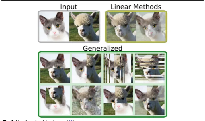
The concept of mixing images in an unintuitive way was further investigated by Summers and Dinneen [66]. They looked at using non-linear methods to combine images into new training instances. All of the methods they used resulted in better performance compared to the baseline models (Fig. 9).

Amongst these non-linear augmentations tested, the best technique resulted in a reduction from 5.4 to 3.8% error on CIFAR-10 and 23.6% to 19.7% on CIFAR-100. In like manner, Liang et  al. [67] used GANs to produce mixed images. They found that the inclusion of mixed images in the training data reduced training time and increased the diversity of GAN-samples. Takahashi and Matsubara [68] experiment

Fig. 7 SamplePairing augmentation strategy [65]

with another approach to mixing images that randomly crops images and concate-nates the croppings together to form new images as depicted below. The results of their technique, as well as SamplePairing and mixup augmentation, demonstrate the sometimes unreasonable effectiveness of big data with Deep Learning models (Fig. 10).

An obvious disadvantage of this technique is that it makes little sense from a human perspective. The performance boost found from mixing images is very difficult to understand or explain. One possible explanation for this is that the increased dataset size results in more robust representations of low-level characteristics such as lines and edges. Testing the performance of this in comparisons to transfer learning and pretrain-ing methods is an interestpretrain-ing area for future work. Transfer learnpretrain-ing and pretrainpretrain-ing are other techniques that learn low-level characteristics in CNNs. Additionally, it will be

Fig. 9 Non-linearly mixing images [66]

interesting to see how the performance changes if we partition the training data such that the first 100 epochs are trained with original and mixed images and the last 50 with original images only. These kinds of strategies are discussed further in Design Consid-erations of Data Augmentation with respect to curriculum learning [69]. Additionally, the paper will cover a meta-learning technique developed by Lemley et al. [37] that uses a neural network to learn an optimal mixing of images.

Random erasing

Random erasing [70] is another interesting Data Augmentation technique developed by Zhong et al. Inspired by the mechanisms of dropout regularization, random erasing can be seen as analogous to dropout except in the input data space rather than embed-ded into the network architecture. This technique was specifically designed to combat image recognition challenges due to occlusion. Occlusion refers to when some parts of the object are unclear. Random erasing will stop this by forcing the model to learn more descriptive features about an image, preventing it from overfitting to a certain visual fea-ture in the image. Aside from the visual challenge of occlusion, in particular, random erasing is a promising technique to guarantee a network pays attention to the entire image, rather than just a subset of it.

Random erasing works by randomly selecting an n × m patch of an image and masking it with either 0 s, 255 s, mean pixel values, or random values. On the CIFAR-10 dataset this resulted in an error rate reduction from 5.17 to 4.31%. The best patch fill method was found to be random values. The fill method and size of the masks are the only parameters that need to be hand-designed during implementation (Figs. 11, 12).

Random erasing is a Data Augmentation method that seeks to directly prevent overfit-ting by altering the input space. By removing certain input patches, the model is forced to find other descriptive characteristics. This augmentation method can also be stacked on top of other augmentation techniques such as horizontal flipping or color filters. Ran-dom erasing produced one of the highest accuracies on the CIFAR-10 dataset. DeVries and Taylor [71] conducted a similar study called Cutout Regularization. Like the random erasing study, they experimented with randomly masking regions of the image (Table 2).

Mikolajcyzk and Grochowski [72] presented an interesting idea to combine random erasing with GANs designed for image inpainting. Image inpainting describes the task of

filling in a missing piece of an image. Using a diverse collection of GAN inpainters, the random erasing augmentation could seed very interesting extrapolations. It will be inter-esting to see if better results can be achieved by erasing different shaped patches such as circles rather than n × m rectangles. An extension of this will be to parameterize the geometries of random erased patches and learn an optimal erasing configuration.

A disadvantage to random erasing is that it will not always be a label-preserving trans-formation. In handwritten digit recognition, if the top part of an ‘8’ is randomly cropped out, it is not any different from a ‘6’. In many fine-grained tasks such as the Stanford Cars dataset [73], randomly erasing sections of the image (logo, etc.) may make the car brand unrecognizable. Therefore, some manual intervention may be necessary depending on the dataset and task.

A note on combining augmentations

Of the augmentations discussed, geometric transformations, color space tions, kernel filters, mixing images, and random erasing, nearly all of these transforma-tions come with an associated distortion magnitude parameter as well. This parameter encodes the distortional difference between a 45° rotation and a 30° rotation. With a large list of potential augmentations and a mostly continuous space of magnitudes, it is easy to conceptualize the enormous size of the augmentation search space. Combining augmentations such as cropping, flipping, color shifts, and random erasing can result in

Fig. 12 Example of random erasing on object detection tasks [70]

Table 2 Results of  Cutout Regularization [104], plus  denotes using traditional augmentation methods, horizontal flipping and cropping

A 2.56% error rate is obtained on CIFAR-10 using cutout and traditional augmentation methods The italic value denote high performance according to the comparative metrics

Method C10 C10+ C100 C100+ SVHN

massively inflated dataset sizes. However, this is not guaranteed to be advantageous. In domains with very limited data, this could result in further overfitting. Therefore, it is important to consider search algorithms for deriving an optimal subset of augmented data to train Deep Learning models with. More on this topic will be discussed in Design Considerations of Data Augmentation.

Data Augmentations based on Deep Learning Feature space augmentation

All of the augmentation methods discussed above are applied to images in the input space. Neural networks are incredibly powerful at mapping high-dimensional inputs into lower-dimensional representations. These networks can map images to binary classes or to n× 1 vectors in flattened layers. The sequential processing of neural networks can be manipulated such that the intermediate representations can be separated from the network as a whole. The lower-dimensional representations of image data in fully-con-nected layers can be extracted and isolated. Konno and Iwazume [74] find a performance boost on CIFAR-100 from 66 to 73% accuracy by manipulating the modularity of neural networks to isolate and refine individual layers after training. Lower-dimensional repre-sentations found in high-level layers of a CNN are known as the feature space. DeVries and Taylor [75] presented an interesting paper discussing augmentation in this feature space. This opens up opportunities for many vector operations for Data Augmentation.

SMOTE is a popular augmentation used to alleviate problems with class imbalance. This technique is applied to the feature space by joining the k nearest neighbors to form new instances. DeVries and Taylor discuss adding noise, interpolating, and extrapolating as common forms of feature space augmentation (Figs. 13, 14).

Fig. 13 Architecture diagram of the feature space augmentation framework presented by DeVries and Taylor [75]

The use of auto-encoders is especially useful for performing feature space augmen-tations on data. Autoencoders work by having one half of the network, the encoder, map images into low-dimensional vector representations such that the other half of the network, the decoder, can reconstruct these vectors back into the original image. This encoded representation is used for feature space augmentation.

DeVries and Taylor [75] tested their feature space augmentation technique by extrapo-lating between the 3 nearest neighbors per sample to generate new data and compared their results against extrapolating in the input space and using affine transformations in the input space (Table 3).

Feature space augmentations can be implemented with auto-encoders if it is necessary to reconstruct the new instances back into input space. It is also possible to do feature space augmentation solely by isolating vector representations from a CNN. This is done by cutting off the output layer of the network, such that the output is a low-dimensional vector rather than a class label. Vector representations are then found by training a CNN and then passing the training set through the truncated CNN. These vector representa-tions can be used to train any machine learning model from Naive Bayes, Support Vec-tor Machine, or back to a fully-connected multilayer network. The effectiveness of this technique is a subject for future work.

A disadvantage of feature space augmentation is that it is very difficult to interpret the vector data. It is possible to recover the new vectors into images using an auto-encoder network; however, this requires copying the entire encoding part of the CNN being trained. For deep CNNs, this results in massive auto-encoders which are very difficult and time-consuming to train. Finally, Wong et al. [76] find that when it is possible to transform images in the data-space, data-space augmentation will outperform feature space augmentation.

Adversarial training

attacks demonstrate that representations of images are much less robust than what might have been expected. This is well demonstrated by Moosavi-Dezfooli et al. [77] using DeepFool, a network that finds the minimum possible noise injection needed to cause a misclassification with high confidence. Su et al. [78] show that 70.97% of images can be misclassified by changing just one pixel. Zajac et  al. [79] cause mis-classifications with adversarial attacks limited to the border of images. The success of adversarial attacks is especially exaggerated as the resolution of images increases.

Adversarial attacking can be targeted or untargeted, referring to the deliberation in which the adversarial network is trying to cause misclassifications. Adversarial attacks can help to illustrate weak decision boundaries better than standard classifica-tion metrics can.

In addition to serving as an evaluation metric, defense to adversarial attacks, adver-sarial training can be an effective method for searching for augmentations.

By constraining the set of augmentations and distortions available to an adversarial network, it can learn to produce augmentations that result in misclassifications, thus forming an effective search algorithm. These augmentations are valuable for strength-ening weak spots in the classification model. Therefore, adversarial training can be an effective search technique for Data Augmentation. This is in heavy contrast to the traditional augmentation techniques described previously. Adversarial augmentations may not represent examples likely to occur in the test set, but they can improve weak spots in the learned decision boundary.

Engstrom et  al. [80] showed that simple transformations such as rotations and translations can easily cause misclassifications by deep CNN models. The worst out of the random transformations reduced the accuracy of MNIST by 26%, CIFAR10 by 72% and ImageNet (Top 1) by 28%. Goodfellow et al. [81] generate adversarial exam-ples to improve performance on the MNIST classification task. Using a technique for generating adversarial examples known as the “fast gradient sign method”, a maxout network [82] misclassified 89.4% of adversarial examples with an average confidence of 97.6%. This test is done on the MNIST dataset. With adversarial training, the error rate of adversarial examples fell from 89.4% to 17.9% (Fig. 15).

Li et al. [83] experiment with a novel adversarial training approach and compare the performance on original testing data and adversarial examples. The results displayed

below show how anticipation of adversarial attacks in the training process can dramati-cally reduce the success of attacks.

As shown in Table 4, the adversarial training in their experiment did not improve the test accuracy. However, it does significantly improve the test accuracy of adversarial examples. Adversarial defense is a very interesting subject for evaluating security and robustness of Deep Learning models. Improving on the Fast Gradient Sign Method, DeepFool, developed by Moosavi-Dezfooli et al. [77], uses a neural network to find the smallest possible noise perturbation that causes misclassifications.

Another interesting framework that could be used in an adversarial training context is to have an adversary change the labels of training data. Xie et al. [84] presented Distur-bLabel, a regularization technique that randomly replaces labels at each iteration. This is a rare example of adding noise to the loss layer, whereas most of the other augmenta-tion methods discussed add noise into the input or hidden representaaugmenta-tion layers. On the MNIST dataset with LeNet [28] CNN architecture, DisturbLabel produced a 0.32% error rate compared to a baseline error rate of 0.39%. DisturbLabel combined with Dropout Regularization produced a 0.28% error rate compared to the 0.39% baseline. To translate this to the context of adversarial training, one network takes in the classifier’s training data as input and learns which labels to flip to maximize the error rate of the classifica-tion network.

The effectiveness of adversarial training in the form of noise or augmentation search is still a relatively new concept that has not been widely tested and understood. Adversarial search to add noise has been shown to improve performance on adversarial examples, but it is unclear if this is useful for the objective of reducing overfitting. Future work seeks to expand on the relationship between resistance to adversarial attacks and actual performance on test datasets.

GAN‑based Data Augmentation

modeling technique that exists; however they are dramatically leading the way in com-putation speed and quality of results.

Another useful strategy for generative modeling worth mentioning is variational auto-encoders. The GAN framework can be extended to improve the quality of samples produced with variational auto-encoders [86]. Variational auto-encoders learn a low-dimensional representation of data points. In the image domain, this translates an image tensor of size height × width × color channels down into a vector of size n × 1, identi-cal to what was discussed with respect to feature space augmentation. Low-dimensional constraints in vector representations will result in a poorer representation, although these constraints are better for visualization using methods such as t-SNE [87]. Imag-ine a vector representation of size 5 × 1 created by an autoencoder. These autoencoders can take in a distribution of labeled data and map them into this space. These classes could include ‘head turned left’, ‘centered head’, and ‘head turned right’. The auto-encoder learns a low-dimensional representation of these data points such that vector operations such as adding and subtracting can be used to simulate a front view-3D rotation of a new instance. Variational auto-encoder outputs can be further improved by inputting them into GANs [31]. Additionally, a similar vector manipulation process can be done on the noise vector inputs to GANs through the use of Bidirectional GANs [88].

The impressive performance of GANs has resulted in increased attention on how they can be applied to the task of Data Augmentation. These networks have the ability to gen-erate new training data that results in better performing classification models. The GAN architecture first proposed by Ian Goodfellow [31] is a framework for generative mode-ling through adversarial training. The best anecdote for understanding GANs is the anal-ogy of a cop and a counterfeiter. The counterfeiter (generator network) takes in some form of input. This could be a random vector, another image, text, and many more. The counterfeiter learns to produce money such that the cop (discriminator network) cannot tell if the money is real or fake. The real or fake dichotomy is analogous to whether or not the generated instance is from the training set or if it was created by the generator network (Fig. 16).

geNet or CIFAR-10. For immediate reference, an ImageNet image is of resolution 256 × 256 × 3, totaling 196,608 pixels, a 250× increase in pixel count compared with MNIST.

Many research papers have been published that modify the GAN framework through different network architectures, loss functions, evolutionary methods, and many more. This research has significantly improved the quality of samples created by GANs. There have been many new architectures proposed for expanding on the con-cept of GANs and producing higher resolution output images, many of which are out of the scope of this paper. Amongst these new architectures, DCGANs, Progressively Growing GANs, CycleGANs, and Conditional GANs seem to have the most applica-tion potential in Data Augmentaapplica-tion.

The DCGAN [91] architecture was proposed to expand on the internal complex-ity of the generator and discriminator networks. This architecture uses CNNs for the generator and discriminator networks rather than multilayer perceptrons. The DCGAN was tested to generate results on the LSUN interior bedroom image data-set, each image being 64 × 64 × 3, for a total of 12,288 pixels, (compared to 784 in MNIST). The idea behind DCGAN is to increase the complexity of the generator network to project the input into a high dimensional tensor and then add volutional layers to go from the projected tensor to an output image. These decon-volutional layers will expand on the spatial dimensions, for example, going from 14 × 14 × 6 to 28 × 28 × 1, whereas a convolutional layer will decrease the spatial dimensions such as going from 14 × 14 × 32 to 7 × 7 × 64. The DCGAN architecture presents a strategy for using convolutional layers in the GAN framework to produce higher resolution images (Figs. 17, 18).

Frid-Adar et  al. [49] tested the effectiveness of using DCGANs to generate liver lesion medical images. They use the architecture pictured above to generate 64 × 64 × 1 size images of liver lesion CT scans. Their original dataset contains 182 CT scans, (53 Cysts, 64 Metastases, and 65 Hemangiomas). After using classical augmentations to achieve 78.6% sensitivity and 88.4% specificity, they observed an increase to 85.7% sen-sitivity and 92.4% specificity once they added the DCGAN-generated samples.

Another architecture of interest is known as Progressively Growing GANs [34]. This architecture trains a series of networks with progressive resolution complexity. These resolutions range from 4 × 4 to 8 × 8 and so on until outputs of size 1024 × 1024 are achieved. This is built on the concept that GANs can accept images as input as well as random vectors. Therefore, the series of GANs work by passing samples from a lower resolution GAN up to higher-resolution GANs. This has produced very amaz-ing results on facial images.

In addition to improving the resolution size of GANs, another interesting architecture that increases the quality of outputs is the CycleGAN [92] proposed by Zhu et al. Cycle-GAN introduces an additional Cycle-Consistency loss function to help stabilize Cycle-GAN training. This is applied to image-to-image translation. Neural Style Transfer [32], dis-cussed further in the section below, learns a single image to single image translation. However, CycleGAN learns to translate from a domain of images to another domain, such as horses to zebras. This is implemented via forward and backward consistency loss functions. A generator takes in images of horses and learns to map them to zebras such that the discriminator cannot tell if they were originally a part of the zebra set or not, as discussed above. After this, the generated zebras from horse images are passed through a network which translates them back into horses. A second discriminator determines if this re-translated image belongs to the horse set or not. Both of these discriminator losses are aggregated to form the cycle-consistency loss.

The use of CycleGANs was tested by Zhu et al. [93] in the task of Emotion Clas-sification. Using the emotion recognition dataset, FER2013 [94], Facial Expression Recognition Database, they build a CNN classifier to recognize 7 different emotions: angry, disgust, fear, happy, sad, surprise, and neutral. These classes are imbalanced and the CycleGAN is used as a method of intelligent oversampling.

CycleGANs learned an unpaired image-to-image translation between domains. An example of the domains in this problem is neutral to disgust. The CycleGAN learns to translate an image representing a neutral image into an image representing the dis-gust emotion (Figs. 19, 20).

Using CycleGANs to translate images from the other 7 classes into the minority classes was very effective in improving the performance of the CNN model on emo-tion recogniemo-tion. Employing these techniquess, accuracy improved 5–10%. To further understand the effectiveness of adding GAN-generated instances, a t-SNE visualiza-tion is used. t-SNE [87] is a visualization technique that learns to map between high-dimensional vectors into a low-high-dimensional space to facilitate the visualization of decision boundaries (Fig. 21).

Another interesting GAN architecture for use in Data Augmentation is Conditional GANs [95]. Conditional GANs add a conditional vector to both the generator and the discriminator in order to alleviate problems with mode collapse. In addition to inputting a random vector z to the generator, Conditional GANs also input a y vector which could be something like a one-hot encoded class label, e.g. [0 0 0 1 0]. This class label targets a specific class for the generator and the discriminator (Fig. 22).

Fig. 19 Some examples of synthetic data created with CycleGANs for emotion classification

Lucic et al. [96] sought out to compare newly developed GAN loss functions. They conducted a series of tests that determined most loss functions can reach similar scores with enough hyperparameter optimization and random restarts. This suggests that increased computational power is a more promising area of focus than algorithmic changes in the generator versus discriminator loss function.

Most of the research done in applying GANs to Data Augmentation and reporting the resulting classification performance has been done in biomedical image analysis

Fig. 21 t-SNE visualization demonstrating the improved decision boundaries when using

CycleGAN-generated samples. a original CNN model, b adding GAN-generated disgust images, c adding GAN-generated sad images, d adding both GAN-generated disgust and sad images [93]

Table 5 Results of ‘Visual Turing Test’ on DCGAN-generated liver lesion images presented by Frid-Adar et al. [139]

Classification accuracy Is ROI real?

Real (%) Synthetic (%) Total score Total score

Expert 1 78 77.5 235\302 = 77.8% 189\302 = 62.5% Expert 2 69.2 69.2 209\302 = 69.2% 177\302 = 58.6%

Table 6 Results of ‘Visual Turing Test’ on  different DCGAN- and WGAN [104]—generated brain tumor MR images presented by Han et al. [140]

Accuracy (%) Real selected as real

Real as synt Synt as real Synt as synt

T1 (DCGAN, 128 × 128) 70 26 24 6 44

Tlc (DCGAN, 128 × 128) 71 24 26 3 47

T2 (DCGAN, 128 × 128) 64 22 28 8 42

FLAIR (DCGAN, 128 × 128) 54 12 38 8 42

Concat (DCGAN, 128 × 128) 77 34 16 7 43

Concat (DCGAN, 64 × 64) 54 13 37 9 41

T1 (WGAN, 128 × 128) 64 20 30 6 44

Tlc (WGAN, 128 × 128) 55 13 37 8 42

T2 (WGAN, 128 × 128) 58 19 31 11 39

FLAIR (WGAN, 128 × 128) 62 16 34 4 46

Concat (WGAN, 128 × 128) 66 31 19 15 35

Concat (WGAN, 64 × 64) 53 18 32 15 35

small probability, GANs are able to reduce the false positive rate of anomaly detection. They do this using the Adversarial Autoencoder framework proposed by Makhzani et al. [98] (Fig. 24).

As exciting as the potential of GANs is, it is very difficult to get high-resolution out-puts from the current cutting-edge architectures. Increasing the output size of the images produced by the generator will likely cause training instability and non-conver-gence. Another drawback of GANs is that they require a substantial amount of data to train. Thus, depending on how limited the initial dataset is, GANs may not be a practical solution. Salimans et al. [99] provide a more complete description of the problems with training GANs.

Neural Style Transfer

Neural Style Transfer [32] is one of the flashiest demonstrations of Deep Learning capabilities. The general idea is to manipulate the representations of images created in CNNs. Neural Style Transfer is probably best known for its artistic applications, but it also serves as a great tool for Data Augmentation. The algorithm works by manipulat-ing the sequential representations across a CNN such that the style of one image can be transferred to another while preserving its original content. A more detailed explanation of the gram matrix operation powering Neural Style Transfer can be found by Li et al. [100] (Fig. 25).

It is important to also recognize an advancement of the original algorithm from Gatys et al. known as Fast Style Transfer [35]. This algorithm extends the loss function from a per-pixel loss to a perceptual loss and uses a feed-forward network to stylize images. This perceptual loss is reasoned about through the use of another pre-trained net. The use of perceptual loss over per-pixel loss has also shown great promise in the applica-tion of super-resoluapplica-tion [101] as well as style transfer. This loss function enhancement enables style transfer to run much faster, increasing interest in practical applications. Additionally, Ulyanov et al. [102] find that replacing batch normalization with instance normalization results in a significant improvement for fast stylization (Fig. 26).

For the purpose of Data Augmentation, this is somewhat analogous to color space lighting transformations. Neural Style Transfer extends lighting variations and enables the encoding of different texture and artistic styles as well. This leaves practitioners of Data Augmentation with the decision of which styles to sample from when deriving new images via Neural Style Transfer.

data into a night-to-day scale, winter-to-summer, or rainy-to-sunny scale. However, in other application domains, the set of styles to transfer into is not so obvious. For ease of implementation, data augmentation via Neural Style Transfer could be done by selecting a set of k styles and applying them to all images in the training set. The work of Style Augmentation [103], avoids introducing a new form of style bias into the dataset by deriving styles at random from a distribution of 79,433 artistic images. Transferring style in training data has been tested on the transition from simulated environments to the real-world. This is very useful for robotic manipulation tasks using Reinforcement Learning because of potential damages to hardware when train-ing in the real-world. Many constraints such as low-fidelity cameras cause these models to generalize poorly when trained in physics simulations and deployed in the real-world.

Tobin et al. [104] explore the effectiveness of using different styles in training simula-tion and achieve within 1.5 cm accuracy in the real-world on the task of object localiza-tion. Their experiments randomize the position and texture of the objects to be detected

Fig. 25 Illustration of style and content reconstructions in Neural Style Transfer [32]

on the table in the simulation, as well as the texture, lighting, number of lights, and ran-dom noise in the background. They found that with enough variability in the training data style, the real-world simply appears as another variation to the model. Interestingly, they found that diversity in styles was more effective than simulating in as realistic of an environment as possible. This is in contrast to the work of Shrivastava et al. [105] who used GANs to make their simulated data as realistic as possible (Fig. 27).

Using simulated data to build Computer Vision models has been heavily investigated. One example of this is from Richter et al. [106]. They use computer graphics from mod-ern open-world games such as Grand Theft Auto to produce semantic segmentation datasets. The authors highlight anecdotes of the manual annotation costs required to build these pixel-level datasets. They mention the CamVid dataset [107] requires 60 min per image to manually annotate, and the Cityscapes dataset [108] requires 90 min per image. This high labor and time cost motivates the use and development of synthetic datasets. Neural Style Transfer is a very interesting strategy to improve the generaliza-tion ability of simulated datasets.

A disadvantage of Neural Style Transfer Data Augmentation is the effort required to select styles to transfer images into. If the style set is too small, further biases could be introduced into the dataset. Trying to replicate the experiments of Tobin et al. [104] will require a massive amount of additional memory and compute to transform and store 79,433 new images from each image. The original algorithm proposed by Gatys et al. [32] has a very slow running time and is therefore not practical for Data Augmentation. The algorithm developed by Johnson et al. [35] is much faster, but limits transfer to a pre-trained set of styles.

Meta learning Data Augmentations

The concept of meta-learning in Deep Learning research generally refers to the concept of optimizing neural networks with neural networks. This approach has become very popular since the publication of NAS [33] from Zoph and Le. Real et al. [109, 110] also

show the effectiveness of evolutionary algorithms for architecture search. Salimans et al. [111] directly compare evolutionary strategies with Reinforcement Learning. Another interesting alternative to Reinforcement Learning is simple random search [112]. Uti-lizing evolutionary and random search algorithms is an interesting area of future work, but the meta-learning schemes reviewed in this survey are all neural-network, gradient-based.

The history of Deep Learning advancement from feature engineering such as SIFT [113] and HOG [114] to architecture design such as AlexNet [1], VGGNet [2], and Inception-V3 [4], suggest that meta-architecture design is the next paradigm shift. NAS takes a novel approach to meta-learning architectures by using a recurrent net-work trained with Reinforcement Learning to design architectures that result in the best accuracy. On the CIFAR-10 dataset, this achieved an error rate of 3.65 (Fig. 28).

This section will introduce three experiments using meta-learning for Data Aug-mentation. These methods use a prepended neural network to learn Data Augmenta-tions via mixing images, Neural Style Transfer, and geometric transformaAugmenta-tions.

Neural augmentation The Neural Style Transfer algorithm requires two parameters for the weights of the style and content loss. Perez and Wang [36] presented an algo-rithm to meta-learn a Neural Style Transfer strategy called Neural Augmentation. The Neural Augmentation approach takes in two random images from the same class. The prepended augmentation net maps them into a new image through a CNN with 5 layers, each with 16 channels, 3 × 3 filters, and ReLU activation functions. The image outputted from the augmentation is then transformed with another random image via Neural Style Transfer. This style transfer is carried out via the CycleGAN [92] exten-sion of the GAN [31] framework. These images are then fed into a classification model and the error from the classification model is backpropagated to update the Neural Augmentation net. The Neural Augmentation network uses this error to learn the opti-mal weighting for content and style images between different images as well as the mapping between images in the CNN (Fig. 29).

Perez and Wang tested their algorithm on the MNIST and Tiny-imagenet-200 data-sets on binary classification tasks such as cat versus dog. The Tiny-imagenet-200 dataset is used to simulate limited data. The Tiny-imagenet-200 dataset contains only 500 images in each of the classes, with 100 set aside for validation. This problem

limits this dataset to 2 classes. Thus there are only 800 images for training. Each of the Tiny-imagenet-200 images is 64 × 64 × 3, and the MNIST images are 28 × 28 × 1. The experiment compares their proposed Neural Augmentation [36] approach with traditional augmentation techniques such as cropping and rotation, as well as with a style transfer approach with a predetermined set of styles such as Night/Day and Winter/Summer.

The traditional baseline study transformed images by choosing an augmentation from a set (shifted, zoomed in/out, rotated, flipped, distorted, or shaded with a hue). This was repeated to increase the dataset size from N to 2 N. The GAN style transfer baseline uses 6 different styles to transform images (Cezanne, Enhance, Monet, Uki-yoe, Van Gogh and Winter). The Neural Augmentation techniques tested consist of three levels based on the design of the loss function for the augmentation net (Con-tent loss, Style loss via gram matrix, and no loss computer at this layer). All experi-ments are tested with a convolutional network consisting of 3 convolutional layers each followed by max pooling and batch normalization, followed by 2 fully-connected layers. Each experiment runs for 40 epochs at a learning rate of 0.0001 with the Adam optimization technique (Table 7).

The results of the experiment are very promising. The Neural Augmentation tech-nique performs significantly better on the Dogs versus Goldfish study and only slightly worse on Dogs versus Cats. The technique does not have any impact on the MNIST problem. The paper suggests that the likely best strategy would be to combine the traditional augmentations and the Neural Augmentations.

Smart Augmentation The Smart Augmentation [37] approach utilizes a similar con-cept as the Neural Augmentation technique presented above. However, the combina-tion of images is derived exclusively from the learned parameters of a prepended CNN, rather than using the Neural Style Transfer algorithm.

Smart Augmentation is another approach to meta-learning augmentations. This is done by having two networks, Network-A and Network-B. Network-A is an augmen-tation network that takes in two or more input images and maps them into a new image or images to train Network-B. The change in the error rate in Network-B is then

backpropagated to update Network-A. Additionally another loss function is incorpo-rated into Network-A to ensure that its outputs are similar to others within the class. Network-A uses a series of convolutional layers to produce the augmented image. The conceptual framework of Network-A can be expanded to use several Networks trained in parallel. Multiple Network-As could be very useful for learning class-specific aug-mentations via meta-learning (Fig. 30).

Smart Augmentation is similar to SamplePairing [65] or mixed-examples in the sense that a combination of existing examples produces new ones. However, the mechanism of Smart Augmentation is much more sophisticated, using an adaptive CNN to derive new images rather than averaging pixels or hand-engineered image combinations.

The Smart Augmentation technique was tested on the task of gender recognition. On the Feret dataset, accuracy improved from 83.52 to 88.46%. The audience dataset responded with an improvement of 70.02% to 76.06%. Most interestingly, results from another face dataset increased from 88.15 to 95.66%. This was compared with traditional augmentation techniques which increased the accuracy from 88.15 to 89.08%. Addition-ally, this experiment derived the same accuracy when using two Network-As in the aug-mentation framework as was found with one Network-A. This experiment demonstrates

Neural + style 0.890

Control 0.840

Quantitative results on dogs vs cats Dogs vs cat

Augmentation Val. acc.

None 0.705

Traditional 0.775

GANs 0.720

Neural + no loss 0.765

Neural + content loss 0.770

Neural + style 0.740

Control 0.710

MNIST 0′s and 8′s

Augmentation Val. acc.

None 0.972

Neural + no loss 0.975

Fig

. 30

I

llustration of the Smar

t A

ug

mentation ar

chit

ec

tur

e [

37

the significant performance increase with the Smart Augmentation meta-learning strat-egy (Fig. 31).

AutoAugment AutoAugment [38], developed by Cubuk et  al., is a much different approach to meta-learning than Neural Augmentation or Smart Augmentation. Auto-Augment is a Reinforcement Learning algorithm [115] that searches for an optimal augmentation policy amongst a constrained set of geometric transformations with mis-cellaneous levels of distortions. For example, ‘translateX 20 pixels’ could be one of the transformations in the search space (Table 8).

In Reinforcement Learning algorithms, a policy is analogous to the strategy of the learning algorithm. This policy determines what actions to take at given states to achieve some goal. The AutoAugment approach learns a policy which consists of many sub-policies, each sub-policy consisting of an image transformation and a magnitude of transformation. Reinforcement Learning is thus used as a discrete search algorithm of augmentations. The authors also suggest that evolutionary algorithms or random search would be effective search algorithms as well.

AutoAugment found policies which achieved a 1.48% error rate on CIFAR-10. Auto-Augment also achieved an 83.54% Top-1 accuracy on the ImageNet dataset. Very inter-estingly as well, the policies learned on the ImageNet dataset were successful when transferred to the Stanford Cars and FGVC Aircraft image recognition tasks. In this case, the ImageNet policy applied to these other datasets reduced error rates by 1.16% and 1.76% respectively.

Geng et al. [116] expanded on AutoAugment by replacing the Reinforcement Learning search algorithm with Augmented Random Search (ARS) [112]. The authors point out that the sub-policies learned from AutoAugment are inherently flawed because of the discrete search space. They convert the probability and magnitude of augmentations into a continuous space and search for sub-policies with ARS. With this, they achieve lower error rates on CIFAR-10, CIFAR-100, and ImageNet (Table 9).

trained with Reinforcement Learning augmentation search performs much better. On the CIFAR-10 dataset this results in 50.99% versus 70.06% accuracy when the models are evaluated on augmented test data.

A disadvantage to meta-learning is that it is a relatively new concept and has not been heavily tested. Additionally, meta-learning schemes can be difficult and time-consuming to implement. Practitioners of meta-learning will have to solve problems primarily with vanishing gradients [118], amongst others, to train these networks.

Sub-policy 7 (Sharpness,0.3,9) (Brightness,0.7,9) Sub-policy 8 (Equalize,0.6,5) (Equalize,0.5,1) Sub-policy 9 (Contrast,0.6,7) (Sharpness,0.6,5) Sub-policy 10 (Color,0.7,7) (TranslateX,0.5,8) Sub-policy 11 (Equalize,0.3,7) (AutoContrast,0.4,8) Sub-policy 12 (TranslateY,0.4,3) (Sharpness,0.2,6) Sub-policy 13 (Brightness,0.9,6) (Color,0.2,8) Sub-policy 14 (Solarize,0.5,2) (Invert,0.0,3) Sub-policy 15 (Equalize,0.2,0) (AutoContrast,0.6,0) Sub-policy 16 (Equalize,0.2,8) (Equalize,0.6,4)

Sub-policy 17 (Color,0.9,9) (Equalize,0.6,6)

Sub-policy 18 (AutoContrast,0.8,4) (Solarize,0.2,8) Sub-policy 19 (Brightness,0.1,3) (Color,0.7,0) Sub-policy 20 (Solarize,0.4,5) (AutoContrast,0.9,3) Sub-policy 21 (TranslateY,0.9,9) (TranslateY,0.7,9) Sub-policy 22 (AutoContrast,0.9,2) (Solarize,0.8,3) Sub-policy 23 (Equalize,0.8,8) (Invert,0.1,3) Sub-policy 24 (TranslateY,0.7,9) (AutoContrast,0.9,1)

Table 9 The performance of ARS on continuous space vs. AutoAugment on discrete space [116]

Model AutoAugment ARS-Aug

Wide-ResNet-28-10 2.68 2.33

Shake-Shake (26 2 × 32 days) 2.47 2.14

Shake-Shake (26 2 × 96 days) 1.99 1.68

Shake-Shake (26 2 × 112 days) 1.89 1.59

AmoebaNet-B (6,128) 1.75 1.49

ing of 50 k samples with 5 k in each class. They also tested with 3 levels of augmentation, no augmentation, original plus same size of generated samples, and original plus double size of generated samples. They found that cropping, flipping, WGAN, and rotation gen-erally performed better than others. The combinations of flipping + cropping and flip-ping + WGAN were the best overall, improving classification performance on CIFAR-10 by + 3% and + 3.5%, respectively.

Design considerations for image Data Augmentation

This section will briefly describe some additional design decisions with respect to Data Augmentation techniques on image data.

Test-time augmentation

In addition to augmenting training data, many research reports have shown the effec-tiveness of augmenting data at test-time as well. This can be seen as analogous to ensem-ble learning techniques in the data space. By taking a test image and augmenting it in the same way as the training images, a more robust prediction can be derived. This comes at a computational cost depending on the augmentations performed, and it can restrict the speed of the model. This could be a very costly bottleneck in models that require real-time prediction. However, test-time augmentation is a promising practice for appli-cations such as medical image diagnosis. Radosavovic et al. [120] denote test-time aug-mentation as data distillation to describe the use of ensembled predictions to get a better representation of the image.

Wang et al. [121] sought out to develop a mathematical framework to formulate test-time augmentation. Testing their test-test-time augmentation scheme on medical image segmentation, they found that it outperformed the single-prediction baseline and drop-out-based multiple predictions. They also found better uncertainty estimation when using test-time augmentation, reducing highly confident but incorrect predictions. Their test-time augmentation method uses a Monte Carlo simulation in order to obtain parameters for different augmentations such as flipping, scaling, rotation, and transla-tions, as well as noise injections.

Perez et al. [122] present a study on the effectiveness of test-time augmentation with many augmentation techniques. These augmentations tested include color augmen-tation, roaugmen-tation, shearing, scaling, flipping, random cropping, random erasing, elastic, mixing, and combinations between the techniques. Table 9 shows the higher perfor-mance achieved when augmenting test images as well as training images. Matsunaga et al. [123] also demonstrate the effectiveness of test-time augmentation on skin lesion classification, using geometric transformations such as rotation, translation, scaling, and flipping.

The impact of test-time augmentation on classification accuracy is another mechanism for measuring the robustness of a classifier. A robust classifier is thus defined as having a low variance in predictions across augmentations. For example, a prediction of an image should not be much different when that same image is rotated 20°. In their experiments searching for augmentations with Reinforcement Learning, Minh et al. [117] measure robustness by distorting test images with a 50% probability and contrasting the accu-racy on un-augmented data with the augmented data. In this study, the performance of the baseline model decreases from 74.61 to 66.87% when evaluated on augmented test images.

Some classification models lie on the fence in terms of their necessity for speed. This suggests promise in developing methods that incrementally upgrade the confidence of prediction. This could be done by first outputting a prediction with little or no test-time augmentation and then incrementally adding test-test-time augmentations to increase the confidence of the prediction. Different Computer Vision tasks require certain con-straints on the test-time augmentations that can be used. For example, image recogni-tion can easily aggregate predicrecogni-tions across warped images. However, it is difficult to aggregate predictions on geometrically transformed images in object detection and semantic segmentation.

Curriculum learning

Aside from the study of Data Augmentation, many researchers have been interested in trying to find a strategy for selecting training data that beats random selection. In the context of Data Augmentation, research has been published investigating the rela-tionship between original and augmented data across training epochs. Some research

In the SamplePairing [65] study, one epoch on ImageNet and 100 epochs on other datasets are completed without SamplePairing before mixed image data is added to the training. Once the SamplePairing images are added to the training set, they run in cycles between 8:2 epochs, 8 with SamplePairing images, 2 without. Jaderberg et al. [124] train exclusively with synthetic data for natural scene text recognition. The synthetic data produced the training data by enumerating through different fonts and augmentation