United Kingdom Vol. IV, Issue 3, March 2016
Licensed under Creative Common Page 234
http://ijecm.co.uk/
ISSN 2348 0386
MONETARY POLICY AND ECONOMIC GROWTH
A CASE STUDY OF IRAN
Seyed Mohammad Alavinasab
Assistant professor of Economics/Faculty of Management & Accounting
College of Farabi, University of Tehran, Iran
Abstract
This study empirically examines the impact of monetary policy on economic growth in Iran over
the period 1971-2011. The time series data for this period are methodologically compatible, so
the variables that are used in the regression are the most appropriate, which allows drawing
valid conclusions. The findings of regression analysis show that in the long run, economic
growth has found to be significantly influenced by money supply, exchange rate and inflation
rate. In short run, the results of estimated Error-correction model indicate that money supply and
exchange rate significantly impact on economic growth.
Keywords: Monetary Policy, Economic Growth, Error Correction Model, Iran
INTRODUCTION
There has been a great resurgence of interest among macroeconomic researchers about the
role of monetary policy. For a long period, it was perceived that monetary policy had no impact
on real economic activity but in late 1980s empirical research in macroeconomics showed that
monetary policy significantly affects the short term course of the real economy (Sims, 1980).
There seems to be a general consensus that changes in aggregate economic activity depend
on how monetary policy is conducted. In other words, macroeconomic aggregates such as
output, employment and prices are affected by the stance of monetary through the monetary
tools, and monetary policy analysts are confronted with the issue of choosing appropriate
measures of the monetary policy stance. This explains why countries establish specialized
institutions, such as the central bank, to formulate and execute appropriate monetary policies for
Licensed under Creative Common Page 235 crucial role in monetary policy in country, particularly, an oil-based economy. Since such an
economy generally suffers from less central bank independence, a monetary expansion
emerges after an increase in oil price. Central bank independence has emerged as one of the
key issues in monetary policy, and during the last two decades, many of the world’s central
banks have been granted more independence. When an economy has central bank
independence and the monetary authority does not follow political orders, policy stability which
is important for a successful monetary policy is guaranteed over time.
Given the crucial role played by monetary policy in pursuit of a sustainable economic
growth, this study intends to investigate the impact of monetary policy on economic growth with
reference to the Iranian economy for the period 1971-2011. The organization of the study is as
follows: Section II contains literature review; methodology is elaborated in section III, section IV
presents empirical results and conclusion are given in section V.
LITERATURE REVIEW
Review of Theoretical Literature
Theoretical literature regarding the ability of monetary policy affecting economic growth can be
argued in two extreme cases:
The Keynesians suggest that change in money supply may affect the level of output
indirectly via interest rate and investment. The monetarists on the other hand believe that
money can affect real variables in the short run but only nominal magnitudes in the long run.
The Keynesian transmission mechanism consisting of three stages is called the cost of
capital channel and is summarized thus: Money → Interest Rate → Investment → Income;
where with the increase in the money supply, interest rate falls and investment and income rise.
The rise in price level raises nominal income that leads to an increase in the transactions and
precautionary demand for money, there by bringing a “feedback effect” on the economy. The
monetarists using the equation of exchange proposed by Irvin Fisher (1911) which is given by
the expression:
MV = PY (1)
Where M is the total quantity of money, P is the price level, V is the velocity of money, and Y is
aggregate income for the economy. Monetarists assume that velocity is constant, and when V is
constant, equation (1) indicates a one-to-one relationship between changes in the money supply
and changes in the value of national income. As a result, equation (1) can be transformed and
shown below:
Licensed under Creative Common Page 236 In this expression, k represents a constant. According to equation (2) changes in output can
only be brought through changes in money supply. Therefore the direct link between the
monetary sector and the real sector of the economy comes from the argument of a constant
velocity. This explains the basis for the monetarist’s argument that changes in monetary policy will impact economic growth. The monetarists who hold that “only money matters”, emphasize
the role of money in explaining short- term changes in national income. They argue that the role
of money has been neglected by Keynesians, if not by Keynes himself. Friedman (1968, 1970
and 1982) has shown that changes in the money supply cause changes in national income.
Suppose the central bank purchased securities in the open market. It raises the price of
securities and lowers the rate of interest. People will therefore start selling securities and hold
more money. People spend their excess money balances on financial assets and durable
consumer goods. Others attracted by low interest rates borrow from banks for expenditure on
houses, durable consumer goods, plants and equipments, etc. These forces tend to increase
aggregate expenditure and income. Monetarists believe that all recessions and depressions are
caused by severe contraction of money and credit, and booms and inflations by excessive
increases in the money supply. The Keynesians who believe that “money does not matter”, reject the monetarist’s view that changes in national income are caused solely by changes in
the money supply. Rather they hold that changes in national income cause changes in the
supply of money. To illustrate, consider an expansionary monetary policy. Suppose the central
bank increases the money supply by open market purchases of Government bonds. It lowers
the interest rate which, in turn, increases investment and expenditure, thereby raising the
national income. The moderate Keynesians still believe like monetarists that hyper-inflations are
caused by excessive money supply. On the other hand, the extreme Keynesians hold that
non-monetary factors like investment cause depressions and booms.
Typically the Keynesians have held that fiscal policy is much more effective policy tool,
and this view was particularly strong in the early years of Keynesianism. At its most extreme the
demand for money was depicted as perfectly interest elastic, a condition known as the liquidity
trap which gives rise to a horizontal LM schedule.
In the IS-LM diagram a horizontal segment of the LM curve happens at a certain
minimum interest rate. Consequently, according to the Keynesians, monetary policy will be
ineffective in influencing on economic growth and changes in the level of output can only be
effected by changes in the IS curve. On the contrary, among the critics of the Keynesians are
the Monetarists who argue that the LM curve is downward sloping as opposed to the horizontal
Licensed under Creative Common Page 237 the LM curve. This makes the monetary policy effective in bringing about changes in economic
growth.
Review of Empirical Literature
Starr (2005) examined the real effects of monetary policy in four core CIS countries namely,
Russia, Ukraine, Belarus, and Kazakhstan using time-series methods and quarterly data from
1995 to 2003. Results show that little evidence of real effects of monetary policy in the four core
CIS countries with the notable exception that interest rates have a significant impact on output
in Russia.
Berument and Dincer (2008) investigated the effects of monetary policy for Turkey using
structural VAR technique, covering the period 1986-2000. The results show that a tight
monetary policy has a temporary effect on output, causing output to decline for three months in
a statistically significant fashion.
Bhuiyan (2008) applied structural VAR model for Canada in order to estimate the effects
of monetary policy shock. The study used the overnight target rate as the policy instrument and
monthly data for the period of 1994-2007. Findings of the study indicate that the transmission of
the monetary policy shock to real output operates through both the interest rate and the
exchange rate.
Nouri & Jafari Samimi (2011) examined the relationship between money supply and
economic growth in Iran adopting Ordinary Least Squares technique and also using data
obtained from the central bank of Iran during 1974 to 2008. To do so, using Levine and Renelt
growth model, and results show that there is a positive and significance relationship between
money supply and economic growth in Iran.
Khosravi & Karimi (2010) investigated the impact of monetary and fiscal policies on
economic growth in Iran using autoregressive distributed approach to co-integration between
1960 and 2006. The empirical results indicated existence of long-run relationship between
economic growth, monetary policy and fiscal policy. The results further showed exchange rate
and inflation as proxies for monetary policy have inverse impact on economic growth.
Lashkary & Hassannezhad Kashani (2011), based on monetarists’ approach examined
neutrality or non-neutrality of the money during the period1959 to 2008 in Iran. Findings show
that there is no significant relationship between the money volume and real economic variables,
production and employment and monetary policies are neutral in Iran. The gross domestic
product in Iran does not fluctuate intensively except in recent years and it has a normal
Licensed under Creative Common Page 238 Moslehi (2006) investigated the effects of monetary and fiscal policies on real and nominal
variables in Iran’s economy based on the analysis during the period 1959 to 2004 applying the
Seemingly Unrelated Regression (SUR). Results confirmed that implementing monetary and
fiscal policies in Iran’s economy cannot influence the real variables. So, their main effects are on
nominal sector of economy or the price levels. Since monetary and fiscal policies are not able to
considerably influence the production changes, it is better to use these policies in relation to
anti-inflationary objectives.
Noferesti (2005) examined the impact of monetary and exchange policies on economy of
Iran, during 1959- 1998. Results indicate that implemented expansionary monetary policies
could affect on real sector of economy and increased level of output and employment. Naeini &
Shiva (1993) tested the Barrow’s theory about money neutrality in Iran’s economy. They found
that the increase in money volume and liquidity does not help production growth and causes
inflationary pressures. Mehrara (1998) found that production in Iran’s economy was an
exogenous variable and money volume played no role in production fluctuations.
RESEARCH METHODOLOGY
To capture the impact of monetary policy on economic growth the empirical equation is based
on the assumption of Keynesian IS – LM function. Therefore, the functional form of the specified
model is suggested as follows:
GDP = f (M2, EXR, IR, INF) (3)
Explicitly, equation 3 can be written as:
GDP = λ0+ λ1 M2 + λ2 EXR + λ3IR + λ4 INF + µ (4)
The log and operational form of the equation 4 is stated thus:
Log GDP = λ0 + λ1LogM2 + λ2LogEX R + λ3LogI R + λ4LogINF + µ (5)
Where: GDP= real gross domestic product, IR = interest rate, M2= broad money supply,
EXR=exchange rate, INF = inflation rate and µ = error term.
The priori expectation: λ1>0; λ2, λ3,λ4<0
The model estimated using annual time series data covering 1971 – 2011, that is forty-one (41)
years and the data were sourced from Time Series Database of Central Bank of Iran.
ESTIMATION AND RESULTS
Unit Root Test
To examine the existence of the long run relationship among variables, stationary analysis by
Licensed under Creative Common Page 239 Table 1: Unit Root Test Result using ADF Procedure
Results Prob. ADF stats Variables First Difference Prob. Adf Stats Variables Level I(1) 0.0109 -4.193418 D(LGDP) 0.7731 -1.598614 LGDP I(1) 0.0293 -3.767269 D(LEXR) 0.9782 -0.523569 LEXR I(1) 0.0000 -6.391375 D(LIR) 0.5513 -2.059656 LIR I(1) 0.0000 -7.079570 D(LINF) 0.0024 -4.758857 LINF I(1) 0.0226 -3.283339 D(LM2) 0.8756 -0.523812 LM2
NOTE: * denotes significance at 5% I (1) Indicates Unit Root in level and Stationary after first difference.
The above table shows that all series are stationary at first difference. This entails that
combination of one or more series way reveal a long run relationship.
Regression Analysis
The long run estimation result shows the presence of autocorrelation in the estimated model.
This implies that the coefficients are no longer efficient. To remove auto correlation,
Autoregressive (AR) and Moving Average (MA) procedure has been used. The following
equation shows the estimated ordinary least square technique:
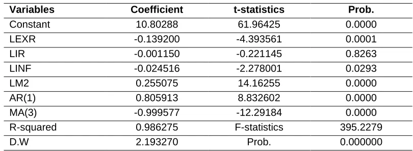
GDP = 10.802 + 0.255 M2 – 0.139 EX R – 0.001 I R – 0.024 INF + 0.805AR (1) – 0.999MA (3)
(6)
Table 2: Long-run Relationship among Variables
Prob. t-statistics Coefficient Variables 0.0000 61.96425 10.80288 Constant 0.0001 -4.393561 -0.139200 LEXR 0.8263 -0.221145 -0.001150 LIR 0.0293 -2.278001 -0.024516 LINF 0.0000 14.16255 0.255075 LM2 0.0000 8.832602 0.805913 AR(1) 0.0000 -12.29184 -0.999577 MA(3) 395.2279 F-statistics 0.986275 R-squared 0.000000 Prob. 2.193270 D.W
Table 2 shows that the effects of all explanatory variables are found with the expected sign.
Money supply (M2) has positive significant impact on economic growth and Variables of
exchange rate (EXR) and inflation rate (INF) have negative significant impact on economic
growth. The coefficient size of M2 is 0.25 percent. Therefore, in this case, one percent change
in money supply will change gross domestic product by 0.25percent. The coefficient size of
Licensed under Creative Common Page 240 percent change in inflation rate and exchange rate will change GDP by 0.024 and 0.139 percent
respectively. The results also indicate that interest rate (IR) has negative and statistically
insignificant relationship with gross domestic product.
Co-integration Test
Johanson co-integration procedure is applied to estimate the long run relation among the
variable in the model. They have two tests statistics for co-integration namely Trace statistics
and Maximum Eigen value statistics. The calculated Trace and Maximum Eigen value test
statistics and their parallel critical value are presented in table 3 and 4.
Table 3: Johansen Co-Integration Test Result (Trace)
Prob.** 5% Critical Value
Trace Statistic Eigen value
Hypothesized
No. of CE(s) 0.803053 105.6192 69.81889 0.0000
None*
0.0819 47.85613
45.50078 0.429926
At most 1
0.1722 29.79707
24.70717 0.329844
At most 2
0.2886 15.49471
9.898139 0.183051
At most 3
0.1200 3.841466
2.417527 0.063250
At most 4
Trace test indicates 1 co-integrating eqn(s) at the 0.05 level. * denotes rejection of the hypothesis at the 0.05 level.
** MacKinnon-Haug-Michelis (1999) p-values.
Table 4: Johansen Co-Integration Test Result (Maximum Eigenvalue)
Prob.** 5% Critical Value
Max-Eigen Statistic Eigen value
Hypothesized
No. of CE(s) 0.803053 6011844 33.87687 0.0000
None*
0.2889 27.58434
20.79361 0.429926
At most 1
0.3025 21.13162
14.80904 0.329844
At most 2
0.4340 14.26460
7.480612 0.183051
At most 3
0.1200 3.841466
2.417527 0.063250
At most 4
Max-eigenvalue test indicates 1 co-integrating eqn(s) at the 0.05 level. * denotes rejection of the hypothesis at the 0.05 level.
** MacKinnon-Haug-Michelis (1999) p-values.
According to probabilities given in Table 3 and 4, the analysis rejects the null hypothesis that
there is no co-integrated vector (None). Results show that both test statistics reject null
hypothesis at 5% level of significance in favor of their alternative that there is one co-integrating
vector. Thus, results from Trace and Maximum Eigen test statistics show that there exists only
Licensed under Creative Common Page 241
Error Correction Model
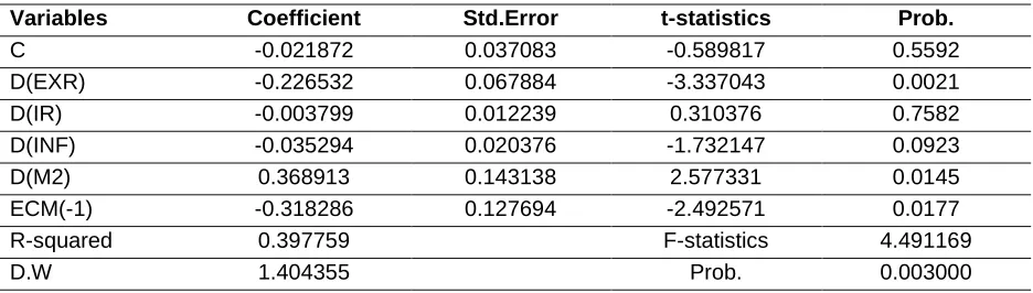
Error Correction Model has been used to test the short run relationship. The estimates in table 5
show that money supply and exchange rate both have significant effect on economic growth in
short run. The coefficient of error correction term has expected negative sign and significant.
The results also indicate that the calculated R2 is 0.397. This implies that about 40% of the total
variation in the GDP is caused by the variations in the explanatory variables while the remaining
60% are caused by factors outside the model, covered by the error term. Furthermore, the DW
statistic suggests that there is evidence of serial autocorrelation.
Table 5: Error Correction Model Estimates
Prob. t-statistics
Std.Error Coefficient
Variables
0.5592 -0.589817
0.037083 -0.021872
C
0.0021 -3.337043
0.067884 -0.226532
D(EXR)
0.7582 0.310376
0.012239 -0.003799
D(IR)
0.0923 -1.732147
0.020376 -0.035294
D(INF)
0.0145 2.577331
0.143138 0.368913
D(M2)
0.0177 -2.492571
0.127694 -0.318286
ECM(-1)
4.491169 F-statistics
0.397759 R-squared
0.003000 Prob.
1.404355 D.W
Stability Analysis
The stability of relationship is imperative for the effectiveness of monetary policies. CUSUM of
recursive residual have been used to check the stability of estimates in the long run.
Figure 1: Test of Stability Analysis
Figure 1 show that the long run estimates of monetary policies with economic growth are stable
Licensed under Creative Common Page 242
Diagnostic Tests
To evaluate the statistical properties of the model in the case of long run, a battery of tests was
performed.
Test for Autocorrelation
To test for autocorrelation in research model, the study makes use of the Breusch-Godfrey
Serial correlation LM test for autocorrelation. As shown in table 6, there is no problem of
autocorrelation in the model as the null of no serial correlation cannot be rejected.
Breusch-Godfrey Correlation LM test indicates that the residuals of the estimated model do not suffer
from autocorrelation.
Table 6: Breusch-Godfrey Serial Correlation LM Test
0.1071 Prob. F(2,31)
2.402521 F-statistic
0.0739 Prob. Chi-Square(2)
5.209508 Obs*R-squared
Heteroskedasticity
This test is basically on the variance of the error term. The test helps to ascertain whether the
variance of the error term is constant. Table 7 shows that the null of homoskedastic residuals
cannot be rejected, and implying that the residuals of the model are homoskedastic.
Table 7: Heteroskedasticity Test: Breusch-Pagan-Godfrey
0.0344 Prob. F(4,35)
2.929712 F-statistic
0.0399 0.0715 Prob. Chi-Square(4)
Prob. Chi-Square(4) 10.03351
8.613483 Obs*R-squared
Scaled explained SS
Normality Test
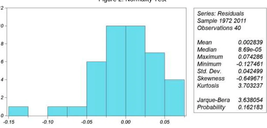
This test is carried out to check whether the error term follow a normal distribution. As shown in
figure 2 the normality test adopted the Jarque-Bera (JB) Test of Normality. Result shows the
residuals are also normally distributed as Jarque-Bera test of normality fails to reject the null of
normally distributed residuals. The same conclusion can be derived using Histogram-Normality
Licensed under Creative Common Page 243 Figure 2: Normality Test
CONCLUSION
The objective of this study is to investigate empirically the impact of monetary policy on
economic growth in Iran between 1971 and 2011. The result of the regression model shows that
in long run, the effects of all explanatory variables are found with the expected sign. Further,
money supply has positive significant impact on economic growth and variables of exchange
rate and inflation rate have negative significant impact on economic growth. While, the effect of
interest rate is negative and statistically is insignificant on gross domestic product. In short run,
the coefficient of ECM has expected negative sign and significant. The estimate of Error
Correction Model shows that money supply and exchange rate both have significant effect on
economic growth. Also, findings show that stability of estimates in the long run and diagnostic
tests indicate that no serial correlation, no heteroskedasticity, and the residuals are normality
distributed.
REFERENCES
Berument, H. and N. Dincer (2008), “Measuring the effects of monetary policy for turkey”, Journal of Economics Cooperation 29 (1), 83-110.
Bhuiyan, R. (2008) “The Effects of Monetary Policy Shocks in a Small Open Economy: A Structural VAR Approach” Queen’s University, Kingston, Ontario, Canada.
Fisher, I. (1911), “The Purchasing Power of Money”, New York: Macmillan, pp. 24-54.
Friedman, M. (1968), “The Role of Monetary Policy”, The American Economic Review 58(1), 1-17.
Licensed under Creative Common Page 244 Friedman. M (1982), “Monetary Policy: Theory and Practice”, Journal of Money, Credit and Banking, February 14, 98-118.
Khosravi A. and Karimi, M. S.(2010), “To Investigation the Relationship between Monetary, Fiscal Policy and Economic Growth in Iran: Autoregressive Distributed Lag Approach to Co-integration”, American Journal of Applied Sciences 7 (3), 415-419.
Lashkary M. and Hassannezhad Kashani B.(2011), “The Impact of Monetary Variables on Economic Growth in Iran: A Monetarists’ Approach”, World Applied Sciences Journal 15 (3), 449-456.
Mehrara, M. (1998), “Interaction between Monetary and Real Sectors in Iran’s Economy”, Journal of Economic Researches in University of Tehran 56, 1-38.
Moslehi, F. (2006), “Effect of Monetary Policies on Iran’s Economy (1959-2004)”, Iran Economic Researches Quarterly 27, 133-151.
Naeini, M.J. and Shiva, R. (1993), “Monetary Policies, Rational Expectations of Production and Inflation”, the Third Seminar in Monetary Policies and exchange Currency.
Noferesti, M. (2005), “Impact of Monetary and Exchange Policy on Economy of Iran in the Framework of a Dynamic Econometric Model”, Journal of Economic Researches, No. 70.
Nouri M. and Jafari Samimi, A. (2011), “The Impact of Monetary Policy on Economic Growth in Iran”, Middle-East Journal of Scientific Research 9 (6), 740-743.
Sims C. A. (1980), “Macroeconomics and Reality”, Economica 48(1), 1- 48.
Starr, M. A. (2005), “Does money matter in the CIS? Effects of monetary policy on output and prices”,
Journal of Comparative Economics 33, 441–461.