Finding The Efficient Set Using The Critical Line Technique And EXCEL

Finding The Efficient Set Using

The Critical Line Technique And EXCEL

John F. Manley, (Email: [email protected]), Iona College

ABSTRACT

This paper extends the discussion of the critical line approach using three risky stocks as described in Haugen’s Modern Investment Theory, 4th edition. A dynamic presentation of the concepts involved in finding the efficient set, using two EXCEL spreadsheets and an HP-12C hand-held calculator, is provided. This dynamic presentation will enable students to understand the composition of the efficient set in a much clearer and effective manner.

INTRODUCTION

t is a challenge to provide a creative way in which to explain the process of determining the efficient set of portfolios to a class of MBA students or advanced undergraduates. This paper begins with a review and then extends the technique for finding the efficient set of portfolios presented by Robert A. Haugen in his popular text, Modern Investment Theory. The extensions discussed in this paper are (1) determining the equation of the critical line by finding and using the weights of two minimum variance portfolios (MVP’s) and (2) using standard optimization techniques to find the global minimum variance portfolio (GMVP). Indeed, GMVP will be one of the two MVP’s used to determine the critical line equation.

\

To accomplish this, a program for the HP-12C calculator is discussed that allows students to determine the variance of any three-stock portfolio. This program will illustrate the portfolio risk to portfolio composition relationship by allowing portfolio weights to change, and how EXCEL may be used successfully in the classroom to take the mystery out of efficient set determination. Spreadsheets may be used to dynamically update many of the parameters of the model – including the covariance matrix, and to show their effect on the location of MVP’s, the critical line, and the efficient frontier.1

Herein, a portfolio is defined as a set of three stocks with weights {W1, W2, W3} as the proportions of

investment funds allocated to each of the three stocks where the weights sum to one. A specific portfolio is identified by the weights assigned the three stocks. Thus, {0.3, 0.4, 0.3} represents one portfolio with 30% invested in stock one, 40% in stock two, and 30% in stock three, while {1.0, 0.6, –0.6} represents another portfolio that involves short selling the third stock so that the combined investment in stocks one and two can exceed available investment funds.

THE MINIMUM VARIANCE AND EFFICIENT SETS

The minimum variance set of portfolios is defined as the collection of portfolios that have the lowest variance, σPP

2

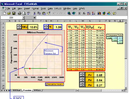
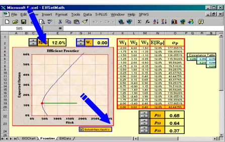
, (or standard deviation, σ) achievable at each given level of expected portfolio return, E[R ], with the available population of stocks. Figure 1 provides a view of the first of two EXCEL spreadsheets used to enhance the presentation of these concepts and shows this minimum variance set as a hyperbolic shaped curve plotted in a Risk-Return relationship using mean-standard deviation (E[R ]-σ) space. The horizontal axis is labeled “Risk” since the standard deviation of the portfolio, σ , is the standard proxy for risk in this context, while the vertical axis is mean

P P

P P P

1

Return. Using Figure 1 as a snapshot of the EXCEL screen on display in the classroom for students to see during the presentation, the horizontal line represents a vast collection of portfolios all of which have an expected portfolio return, E[R ], equal to 10%. However, only one of these many portfolios, represented by the leftmost point on this horizontal line, is a member of the minimum variance set.

P

The top half of the minimum variance set of portfolios is called the efficient set of portfolios. These points are the points on the hyperbolic shaped curve in Figure 1 above the point labeled GMVP where its slope changes from negative to positive. The efficient set of portfolios is defined as the collection of portfolios which have the highest attainable expected portfolio rate of return, E[RP], at each given level of risk or standard deviation, σP.

ISOEXPECTED RETURN LINES

Haugen discusses an isoexpected return line in Chapter 5 of Modern Investment Theory. In this paper, the three expected returns are kept constant throughout the discussion at E[R1] = 5%, E[R2] = 10%, and E[R3] = 15%. All

other data may be dynamically updated using EXCEL in a classroom presentation. In Figure 1, the horizontal line represents all portfolios that have the same expected return, namely 10% in this figure. The students should note the diamond shaped point superimposed on this horizontal line. This point represents one of the many portfolios with E[RP] = 10%. In particular, this is the Portfolio {1.0, –1.0, 1.0}. A table is also displayed containing a selection of

other portfolios each of which has an E[RP] = 10% as shown in column four. One of these, in row 13, is the Portfolio

{1.0, –1.0, 1.0.} represented by the diamond shaped point. Haugen’s discussion includes how the weights of every

portfolio with E[RP] = 10% are determined. For a three-stock portfolio, the equation for expected portfolio return is

given by

E[RP] = W1 E[R1] + W2 E[R2] + W3 E[R3]. (1)

Since W3 = 1 – W1 – W2, we can rewrite this equation as

E[RP] = W1 E[R1] + W2 E[R2] + (1 – W1 – W2) E[R3]. (1’)

We can now solve this equation for W2 as a function of W1, which is given as follows:

W2 = ((E[R3] – E[R1])/(E[R2] – E[R3])) W1 + ((E[RP] – E[R3])/(E[R2] – E[R3])). (1’’)

Since we have assumed that the expected returns for the three stocks are given as: E[R1] = 5%, E[R2] = 10%, and

E[R3] = 15%, then this equation becomes

W2 = –2.0 W1 + (E[RP] – 0.15)/( –0.05). (2)

This is the equation of a straight line called an isoexpected return line in W1-W2 space. Each point on the

line, with coordinates (W1, W2), represents a portfolio {W1, W2, W3 = 1 – W1 – W2} with the same expected portfolio

return, E[RP]. For a given E[RP], we obtain a relation that must hold between W1 and W2 if the portfolio is to have

that given value of E[RP]. For example, given E[RP] = 10%, then W2 = –2.0 W1 + 1.0. Therefore, to find the

weights of any portfolio with E[RP] = 10%, begin by choosing a value for W1, while setting W2 = –2.0 W1 + 1.0, and

W3 = 1 – W1 – W2. For example, choosing W1 = 1.0, requires that W2 = –1.0, and that W3 = 1.0. Thus, the Portfolio

{1.0, –1.0, 1.0} will have an expected return equal to 10%.

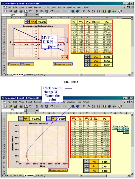
This isoexpected return line is plotted in W1-W2 space in Figure 2, the second of EXCEL spreadsheets.

Notice that the same table shown in Figure 1 is displayed in Figure 2. Students may identify in a clearer fashion how the entries in the first four columns of this table are derived using the process explained above after assuming a value for the weight invested in stock one, W1. Except for the last row, selected values for W1 are chosen (from –2.0 to 2.0

in this example) and placed in column one. The values for W2 shown in column two are computed from W2 = –2.0

reported in column four, are computed from equation (1), E[RP] = W1 (0.05) + W2 (0.10) + W3 (0.15). These are each

equal to E[RP] = 10% as expected.

PORTFOLIO STANDARD DEVIATION

The last column in the table contains the standard deviation of each of these several portfolios. For a three-stock portfolio, the equation for variance is given by

σPP

2

= W12σ12 + W22σ22 + W32σ32 + 2 W W1 2σ12 + 2 W W1 3σ13 + 2 W W2 3σ23 (3)

where σi2 = VAR(Ri) and σij = COV[Ri, Rj]. The standard deviation of a portfolio, σP, is the square root of the

portfolio variance, σPP

2

, calculated in (3). Initially, using the values contained in the covariance table of Figure 1, namely σ12 = 0.25, σ22 = 0.21, σ32 = 0.28, σ = 0.15, σ = 0.17, and σ = 0.09, as inputs into equation (3), we find

that the standard deviation of the Portfolio {1.0, –1.0, 1.0} is σ = 77.4597%. This is the portfolio in Figure 1 represented by the diamond shaped point superimposed on the horizontal line at the level E[R ] = 10%. Note that, although each of the portfolios in this table has the same expected return, E[R ] = 10%, they all have different standard deviations as shown in column five. At the top and bottom of the table, the standard deviations in column five are large. In the middle of the table they are smaller. Only one of the portfolios with an E[R ] = 10% is a member of the minimum variance set. In Figure 1, this is the portfolio at the leftmost point along the horizontal line at the level E[R ] = 10%. In Figure 2, this portfolio is the portfolio on the isoexpected return line designated by the circular point. Since it is a member of the minimum variance set, we call it a minimum variance portfolio (MVP). It is the only portfolio at E[R ] = 10% that is a member of the minimum variance set.

12 13 23 P P P P P P

At this point, students may be asked to select several portfolios whose expected returns are equal to 10% to calculate the standard deviation of these portfolios using the method described above. To aid students to accomplish this task efficiently, the instructor may distribute a program that runs on the HP-12C hand-held calculator to the students. This program should calculate the standard deviation of any three-stock portfolio.

Since the value of W1 determines the values of W2 and W3, the EXCEL spreadsheet shown in Figure 1 has a

feature built into it, just above the plot, that allows W1 to vary over the range –2.0 to 2.0 in steps of 0.10. As this

value is varied as input by the instructor, students may watch the location of the portfolio represented by the diamond shaped point move along the horizontal line positioned at the 10% level of portfolio expected return. As W1 is

decremented from 2.0, the point moves first to the left, touches the minimum variance set line when W1 is between

0.20 and 0.30 (as shown in Figure 3) and then moves back to the right as W1 continues down to –2.0. A quick glance at the table confirms that the MVP at the 10% expected return level has a value of W1 that is in the neighborhood of

0.25. It should be emphasized that these portfolios, on the horizontal line in Figure 1, are the same portfolios that lie on the isoexpected return line shown for E[RP] = 10% in Figure 2. Also, in Figure 2, the MVP, designated by the

circular point on the isoexpected return line, has a W1 coordinate that is approximately 0.25.

After this exercise, students may be asked to calculate the exact weights of the MVP at the 10% expected return level. There is an alternative to the method of Lagrangian Multipliers Haugen uses in his Appendix 3. Students may be instructed to substitute the two required constraints, namely, W2 = –2.0 W1 + 1.0, (required for the portfolio to

have an expected return equal to 10%), and W3 = 1 – W1 – W2, (such that the portfolio weights sum to 1.0), into

equation (3). This will obtain the following variance equation, which is a function of W1 only:

σPP

2

= (σ12 + 4.0 σ22 + σ32 – 4.0 σ12 + 2.0 σ13 – 4.0 σ23) W12 + (2.0σ12 + 2.0σ23 – 4.0 σ22) W + 1 σ22. (3’)

Setting the first derivative of equation (3’), dσPP

2

/dW , equal to zero, students may be shown how to solve for the MVP weight for the first stock, W *, as well as the remaining MVP weights, W * = –2.0 W * + 1.0 and W * = 1 – W * – W *. For the default values contained in the covariance table shown in Figure 1, we obtain the results W * = 0.24, W * = 0.52, and W * = 0.24 for E[R ] = 10%. At the very bottom of the table in Figures 1 and 2, in the last row of the table, these weights for the MVP at E[R ] = 10% are displayed. This MVP, {0.24, 0.52, 0.24}, has a standard deviation, σ , equal to 40.8412%. By definition, no other portfolio with E[R ] = 10% has a lower standard deviation.

1

1 2 1 3

1 2 1

2 3 P

P

This entire exercise – finding the MVP at a given level of E[RP] – is an important step for students in the

process of understanding the identification the efficient set. Students should be encouraged to repeat this process for other values of E[RP], such as E[RP] = 15%, till they are comfortable with the concepts and the calculations. In this

regard, another key feature of these two EXCEL spreadsheets is that E[RP] can be dynamically changed via the

control labeled E[RP] at the top of both spreadsheets. This changes the value of E[RP] in steps of 0.5% and updates

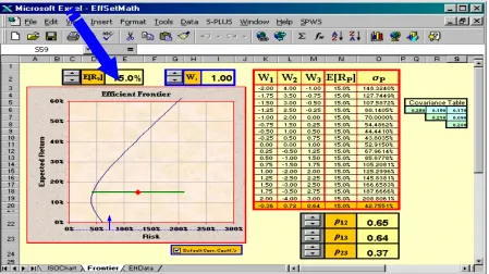
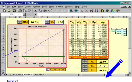
everything in both spreadsheets that depend on E[RP]. Note that, when E[RP] is changed to 15%, the horizontal line

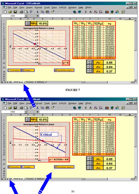
from Figure 1 moves up to E[RP] = 15% as shown in Figure 4. Also, the isoexpected return line from Figure 2 shifts

to the left, parallel to its original position, as shown in Figure 5. Students should be encouraged to recognize that the shift is parallel because, for a given set of three expected returns, E[R1], E[R2], and E[R3], isoexpected return lines all

have the same slope. Equation (2) shows that, for the data being used in this paper, the slope is equal to –2.0 and that only the W2–intercept changes as E[RP] is changed. Also, except for W1 in column one, all the entries in the table

change to reflect the fact that the equation of the isoexpected return line has changed to W2 = – 2.0 W1 for E[RP] =

15% and that the MVP at E[RP] = 15% is now {–0.36, 0.72, 0.64}. The circular point on the isoexpected return line in

Figure 5 also shifts to a new position to reflect the fact that the MVP at E[RP] = 15% has (W1, W2) coordinates (–0.36,

0.72) in W1-W2 space. Students can observe all of these changes, either before or after attempting to find the MVP at

E[RP] = 15%, in order to reinforce their understanding of the process. The instructor may note, at the bottom left hand

corner of Figure 5, that the option of showing an entire family of isoexpected return lines is available by checking the box labeled “Families.” When checked, the display shown in Figure 6 appears on the screen and students can now more readily appreciate the fact that these isoexpected return lines are a set of parallel lines in W1-W2 space whose

position is determined by the value of E[RP].

THE CRITICAL LINE

At this point it should be clear that, given any level of E[RP], the exact weights of the MVP at that level can

be found. However, there are an infinite number of such levels of E[RP] and, therefore, infinite such MVP’s. The

instructor may describe and demonstrate the method discussed by Haugen for finding all of them; that is, how the minimum variance set is found. The circular point on Figures 2 and 5, which is superimposed on the isoexpected return line, represents the (W1, W2) coordinates of the MVP at whatever level of E[RP] is selected. This point shifts in

position as E[RP] is changed from 10% to 15%. As it shifts, a careful observer may notice that it traces out a straight

line in W1-W2 space! This straight line is what Haugen calls the critical line. It shows the portfolio weights of every

portfolio in the minimum variance set. 2

Students may visualize a straight line being traced out by the circular point as E[RP] is slowly changed from

10% to 15%. (See Figure 5) However, to allow the actual clear observation of this fact, the instructor can now check the box labeled “Critical Line” in the lower left-hand corner of Figures 2 and 5. This displays the critical line on the screen, as shown in Figure 7. Now, if the process of incrementing E[RP] over the range 10% to 15% is repeated,

students will explicitly observe that the circular point follows the path of the critical line. Of course, the “Families” box may or may not be checked at the same time at the discretion of the presenter.

Now that we have observed that the (W1, W2) coordinates of every MVP lie on a straight line in W1-W2

space, it would seem that a logical progression would be to determine the equation of this critical line. Although he clearly states that finding the minimum variance set is equivalent to finding the location of the critical line, Haugen’s presentation does not extend to this point. How better to find the location of a line than to determine its equation! This is what we will do now to extend the discussion of finding the efficient set. To determine the equation of a straight line, we need only find two points on the line. But we have already done this. For the data we have been using thus far, we have found that the (W1, W2) coordinates of two different MVP’s on the critical line are (0.24, 0.52)

and (–0.36, 0.72). Students may now find the equation of the critical line in W1-W2 space. Both of these points,

which can be used to determine the equation of the critical line, are interesting points because they represent the (W1,

W2) coordinates of two different MVP’s. However, there is an even more interesting point that can be used in place of

2

either one of these two and that is the point representing the (W1, W2) coordinates of the global minimum variance

portfolio (GMVP). Therefore, we will first determine the (W1, W2) coordinates of the GMVP and then use them to

find the equation of the critical line.

To find the weights of the GMVP, we need to again minimize portfolio variance, σPP

2

, but this time without placing any constraint on E[R ]. Thus, we substitute just one constraint, namely, W = 1 – W – W , such that the portfolio weights sum to 1.0, into equation (3) to obtain the following variance equation:

P 3 1 2

σPP

2

= (σ12 + σ32 – 2.0 σ13)W12 + (σ22 + σ32 – 2.0 σ23)W22 + (2.0 σ32 + 2.0 σ – 2.0 σ – 2.0 σ )W W + (2.0 σ – 2.0

σ32)W + (2.0 1 σ23 – 2.0 σ32)W + 2 σ32. (4) 12 13 23 1 2 13

Since this is a function of both W1 and W2, we next set the two first partial derivatives, δσPP

2

/δW and

δσ 2 1

PP/δW2 equal to zero to solve simultaneously for W1** and W2**, the GMVP weights for the first and second stock. Then, W3** = 1 – W1** – W2**. For the default values contained in the covariance table shown in Figure 1,

we obtain the results W1** = 0.06, W2** = 0.58, and W3** = 0.36. Using these weights, we find that E[RP]** =

11.5% and that σP** = 40.3980%. If, on the first EXCEL spreadsheet, we now use the spinner to set E[RP] = 11.5%

(as shown in Figure 8), then the weights and standard deviation of the GMVP will be displayed in the last row of the table. And the extreme left-hand point of the horizontal line positioned at the level E[RP] = 11.5% in the plot will

represent the GMVP. This GMVP, {0.06, 0.58, 0.36}, has the lowest possible standard deviation of any portfolio that can be constructed with the three stocks we have been using in this paper for illustrative purposes. We can now use the (W1, W2) coordinates of the GMVP {0.06, 0.58, 0.36} and of the MVP at E[RP] = 10% {0.24, 0.52, 0.24} to

determine the equation of the critical line, which is W2 = 0.60 – (1/3) W1. (Critical Line Equation) (5)

Note that when the critical line is displayed on the EXCEL spreadsheet, as it is in Figure 7, its equation is displayed in the lower right-hand corner of the plot. Also note that the (W1, W2) coordinates of the MVP at E[RP] = 15%, {– 0.36,

0.72, 0.64}, satisfy this equation.

THE EFFICIENT SET

One of the primary benefits of having determined the equation of the critical line is that we can now specify exactly the weights of every member of the efficient set. The efficient set is the set of all portfolios defined by {{W1,

W2, W3}| W1≤ 0.06, W2 = 0.60 –(1/3) W1, W3 = 1 – W2 – W3}. W1 ≤ 0.06 guarantees that the portfolios will be

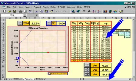
members of the top half of the minimum variance set, which we defined earlier as the efficient set, since those portfolios with W1≤ 0.06 have E[RP] ≥ 11.5%. For example, the portfolio {0.0, 0.60, 0.40} with E[RP] = 12% is a

member of the efficient set. Using the spinner to set E[RP] = 12% makes this clear, as is shown in Figure 9, where the

portfolio in the last row of the table, which contains the MVP weights at the level E[RP] = 12%, is the portfolio {0.0,

0.60, 0.40}.

An additional benefit from having the equation of the critical line is that examples that are used to illustrate important properties of the minimum variance set can now be constructed with numbers that correctly correspond to the data for the three stocks being used to form the portfolios. Haugen states Property I as: By combining two or more portfolios in the minimum variance set, we get another portfolio in the minimum variance set. He then constructs an example using two portfolios, namely portfolio 1: {–1.50, 1.20, 1.30} and portfolio 3: {0.00, 0.70, 0.30}, neither of which is a member of the minimum variance set. Investing $1,000 in each of these two portfolios results in portfolio 2: {-0.75, 0.95, 0.80}, a portfolio which is also not a member of the minimum variance set.

By using the critical line equation, we know that given W1 = –1.50, portfolio 1 should be {–1.50, 1.10, 1.40}.

Given W1 = 0.00, portfolio 3 should be {0.00, 0.60, 0.40}. Investing $1,000 in each of these two portfolios results in

DYNAMICALLY UPDATING THE COVARIANCE MATRIX

We illustrate how changing the values of the three covariances in the covariance table changes the shape of the minimum variance set and the location of the critical line (plotted in the two different EXCEL spreadsheets that we have been using). To change the values in the covariance table, we change the correlation coefficients ρ12, ρ13, and

ρ23. These correlation coefficients are displayed with their individual controls in the lower right-hand corner of both

spreadsheets. For students, this is quite a valuable demonstration of how the location of the efficient set critically depends on how the various stocks in the portfolio are correlated.

Recall that we keep the values of E[R1], E[R2], and E[R3] constant at 5.0%, 10.0%, and 15.0% respectively;

also note that there is a box labeled “Default Corr. Coeff’s”. When checked, the values of the correlation coefficients are set such that the three covariances assume the default values of σ12 = 0.15, σ13 = 0.17, and σ23 = 0.09, namely, the

values that we have been using in the paper up to this point. By removing the check mark, the correlation coefficients are free to be varied by the presenter. We will illustrate three such variations to make three different points.

First, in Figures 10 and 11, the correlation coefficients have been changed to ρ12 = –0.07, ρ13 = 0.14, and ρ23

= –0.62. With the first and third stocks negatively correlated with the second stock, the minimum variance set, in the vicinity of the GMVP, bulges more toward the left in the direction of lower portfolio standard deviation and, hence, lower risk. In this case, the weights of the GMVP become W1** = 0.1369, W2** = 0.4790, and W3** = 0.3841. With

these weights, RP** = 11.24% and σP** = 20.19%. The point being demonstrated is that introducing negative

correlation between stocks in a portfolio allows one to create portfolios with previously unattainable lower risk. Notice also that the equation of the critical line, displayed in Figure 11, changes such that its slope is less negative. This indicates that, as we move along the minimum variance set, the proportion of funds invested in the second stock does not vary nearly as much as it does for stocks one and three.

Next, in Figures 12 and 13, the correlation coefficients have been changed to ρ12 = 0.98, ρ13 = 0.85, and ρ23 =

0.90. Now, with all three stocks highly positively correlated, the minimum variance set is quite steep to the point of being almost vertical. In this case, the weights of the GMVP become W1** = –1.6188, W2** = 3.0111, and W3** = –

0.3923. With these weights, RP** = 16.13% and σP** = 42.37%. With these correlation coefficients, another

important point can now be demonstrated by examining the critical line in Figure 13. Define a triangle in this space with vertices at (0.0, 0.0), (0.0, 1.0), and (1.0, 0.0). Such a triangle is superimposed on the plot in Figure 13. Notice that, in the case being discussed here, the critical line does not pass through this triangle, as illustrated in Figure 13. This indicates that every portfolio in the minimum variance set requires short selling at least one stock in the portfolio. As a result, the minimum variance sets, with and without shortselling permitted, nowhere coincide and is discussed thoroughly in Haugen’s text. Our pedagogical point is that these EXCEL spreadsheets allow the demonstration of many important points discussed in this paper and in Haugen’s text.

Finally, in Figures 14 and 15, the correlation coefficients have again been changed, this time to ρ12 = 0.27,

ρ13 = 0.66, and ρ23 = –0.71. The point here is to demonstrate that there are certain sets of correlation coefficients,

which give rise to portfolios that cannot exist in reality in that their variances would be negative. A case in point, in this instance, is the portfolio {–1.50, 1.50, 1.00}. Using equation (3) to calculate portfolio variance gives the result

σPP

2

= –0.0037. In both figures 14 and 15, this results in having the EXCEL notation #NUM! placed in the cell where the portfolio standard deviation would have appeared.

CONCLUSION

Students often have difficulty visualizing how the relationships among individual stocks determine the location of the efficient set in σP-RP space. Robert Haugen’s presentation of this topic in a three-stock-world context

We have also used a program for the HP-12C hand-held calculator, which calculates the variance of any three-stock portfolio. This program gives students the ability to get involved in the presentation by permitting them to quickly calculate portfolio standard deviations, which they can use to check their knowledge of the concepts being covered.

In the future, this presentation will be further developed to include dynamic changing of the stocks’ expected returns. It will also include a display of the three two-stock combination lines and of the efficient frontier as it would look if short selling were not permitted. This added display will also automatically update as the input data changes, much the way the current display updates now in response to input changes.

REFERENCES

1. Haugen, Robert A. (1997). Modern Investment Theory, 4th ed., Upper Saddle River, N J, Prentice Hall.

FIGURE 1

Minimum Variance Set

FIGURE 2

MVP for

E[RP] =

10%

FIGURE 3

Click here to change W1 –

FIGURE 4

FIGURE 6

FIGURE 7

FIGURE 8

GMV

FIGURE 10

FIGURE 11

FIGURE 12

FIGURE 13

FIGURE 14

?