Learning Text Pair Similarity with Context-sensitive Autoencoders
Hadi Amiri1, Philip Resnik1, Jordan Boyd-Graber2, Hal Daum´e III1 1Institute for Advanced Computer Studies
University of Maryland, College Park, MD 2Department of Computer Science University of Colorado, Boulder, CO
{hadi,resnik,hal}@umd.edu,jordan.boyd.graber@colorado.edu
Abstract
We present a pairwise context-sensitive Autoencoderfor computing text pair sim-ilarity. Our model encodes input text into context-sensitive representations and uses them to compute similarity between text pairs. Our model outperforms the state-of-the-art models in two semantic re-trieval tasks and a contextual word simi-larity task. For retrieval, our unsupervised approach that merely ranks inputs with re-spect to the cosine similarity between their hidden representations shows comparable performance with the state-of-the-art su-pervised models and in some cases outper-forms them.
1 Introduction
Representation learning algorithms learn repre-sentations that reveal intrinsic low-dimensional structure in data (Bengio et al., 2013). Such rep-resentations can be used to induce similarity tween textual contents by computing similarity be-tween their respective vectors (Huang et al., 2012; Silberer and Lapata, 2014).
Recent research has made substantial progress on semantic similarity using neural networks (Rothe and Sch¨utze, 2015; Dos Santos et al., 2015; Severyn and Moschitti, 2015). In this work, we focus our attention on deep autoencoders and extend these models to integrate sentential or documentcontext information about their inputs. We represent context information as low dimensional vectors that will be injected to deep autoencoders. To the best of our knowledge, this is the first work that enables integrating context into autoencoders.
In representation learning, context may appear in various forms. For example, the context of
a current sentence in a document could be ei-ther its neighboring sentences (Lin et al., 2015; Wang and Cho, 2015), topics associated with the sentence (Mikolov and Zweig, 2012; Le and Mikolov, 2014), the document that contains the sentence (Huang et al., 2012), as well as their com-binations (Ji et al., 2016). It is important to inte-grate context into neural networks because these models are often trained with only local informa-tion about their individual inputs. For example, recurrent and recursive neural networks only use local information about previously seen words in a sentence to predict the next word or composition.1 On the other hand, context information (such as topical information) often capture global informa-tion that can guide neural networks to generate more accurate representations.
We investigate the utility of context informa-tion in three semantic similarity tasks: contextual word sense similarityin which we aim to predict semantic similarity between given word pairs in their sentential context (Huang et al., 2012; Rothe and Sch¨utze, 2015),question rankingin which we aim to retrieve semantically equivalent questions with respect to a given test question (Dos Santos et al., 2015), andanswer rankingin which we aim to rank single-sentence answers with respect to a given question (Severyn and Moschitti, 2015).
The contributions of this paper are as follows: (1) integrating context information into deep au-toencoders and (2) showing that such integra-tion improves the representaintegra-tion performance of deep autoencoders across several different seman-tic similarity tasks.
Our model outperforms the state-of-the-art
su-1For example, RNNs can predict the word “sky” given the sentence “clouds are in the ,” but they are less accurate when longer history or global context is required, e.g. pre-dicting the word “french” given the paragraph “I grew up in France. . . . I speak fluent .”
pervised baselines in three semantic similarity tasks. Furthermore, the unsupervised version of our autoencoder show comparable performance with the supervised baseline models and in some cases outperforms them.
2 Context-sensitive Autoencoders
2.1 Basic Autoencoders
We first provide a brief description of basic au-toencoders and extend them to context-sensitive ones in the next Section. Autoencoders are trained using a local unsupervised criterion (Vincent et al., 2010; Hinton and Salakhutdinov, 2006; Vincent et al., 2008). Specifically, the basic autoencoder in Figure 1(a) locally optimizes the hidden represen-tationh of its inputxsuch thathcan be used to accurately reconstructx,
h=g(Wx+bh) (1)
ˆ
x=g(W0h+b ˆ
x), (2)
wherexˆis the reconstruction ofx, the learning pa-rametersW ∈Rd0×d
andW0 ∈Rd×d0
are weight matrices,bh ∈Rd0 andbxˆ ∈Rdare bias vectors for the hidden and output layers respectively, and
gis a nonlinear function such astanh(.).2 Equa-tion (1)encodesthe input into an intermediate rep-resentation and Equation (2)decodesthe resulting representation.
Training a single-layer autoencoder corre-sponds to optimizing the learning parameters to minimize the overall loss between inputs and their reconstructions. For real-valued x, squared loss is often used, l(x) = ||x−xˆ||2, (Vincent et al., 2010):
min
Θ
n X
i=1
l(x(i))
Θ={W,W0,b
h,bxˆ}.
(3)
This can be achieved using mini-batch stochastic gradient descent (Zeiler, 2012).
2.2 Integrating Context into Autoencoders
We extend the above basic autoencoder to inte-grate context information about inputs. We as-sume that—for each training examplex ∈ Rd—
we have a context vector cx ∈ Rk that contains
contextual information about the input.3 The na-2If the squared loss is used for optimization, as in Equa-tion (3), nonlinearity is often not used in EquaEqua-tion (2) (Vin-cent et al., 2010).
3We slightly abuse the notation throughout this paper by referring tocxorhias vectors, not elements of vectors.
𝒉
𝒙 𝑾 𝒙
𝑾′
^
(a) Basic Autoencoder
𝒉
𝒙 𝑾 𝑾′
𝒙^
𝑽
𝒉𝒄
^ 𝒉𝒄
𝑽′
[image:2.595.323.514.61.165.2](b) Context Autoencoder
Figure 1: Schematic representation of basic and context-sensitive autoencoders: (a) Basic autoen-coder maps its input x into the representation h
such that it can reconstructxwith minimum loss, and (b) Context-sensitive autoencoder maps its in-putsxandhcinto a context-sensitive
representa-tionh (hcis the representation of the context
in-formation associated tox).
ture of this context vector depends on the input and target task. For example, neighboring words can be considered as the context of a target word in contextual word similarity task.
We first learn the hidden representation hc ∈
Rd0
for the given context vector cx. For this, we
use the same process as discussed above for the basic autoencoder where we use cx as the input
in Equations (1) and (2) to obtainhc. We then use
hcto develop our context-sensitive autoencoder as
depicted in Figure 1(b). This autoencoder maps its inputsxandhcinto acontext-sensitive
represen-tationhas follows:
h=g(Wx+Vhc+bh) (4)
ˆ
x=g(W0h+bxˆ) (5)
ˆ
hc=g(V0h+bˆhc). (6)
Our intuition is that ifhleads to a good recon-struction of its inputs, it has retained information available in the input. Therefore, it is a context-sensitive representation.
The loss function must then compute the loss between the input pair (x,hc) and its
reconstruc-tion (xˆ, hˆc). For optimization, we can still use
squared loss with a different set of parameters to minimize the overall loss on the training examples:
l(x,hc) =||x−xˆ||2+λ||hc−hˆc||2
min
Θ
n X
i=1
l(x(i),h(i)
c )
𝒄𝑥 𝑽0
h1
hc 𝒙 𝑾1 𝑽1
hi-1
hi 𝑾𝑖
hc 𝑽𝑖
DAE-i
DAE-1
hc
DAE-0
(a) Network initialization
h1
hn
hc
𝒙 𝒄𝑥
𝑽0 𝑾1
𝑾𝑛 𝑽𝑛
𝑽1
𝑓𝜃(𝒙)
(b) Stacking Denoising Autoencoders
hc
𝒙 𝒄𝑥
hc
𝑽0
Encode
r
Deco
der
𝑾1 𝑾𝑛 𝑽1
𝑽𝑛
𝑾𝑛𝑇 𝑾1𝑇
𝑽𝑛𝑇 𝑽1𝑇 𝑽0𝑇
𝒙 ^ 𝒄𝑥
^
^
[image:3.595.80.525.60.224.2](c) Unrolling and Fine-tuning
Figure 2: Proposed framework for integrating context into deep autoencoders. Context layer (cxandhc)
and context-sensitive representation of input (hn) are shown in light red and gray respectively. (a)
Pre-training properly initializes a stack of sensitive denoising autoencoders (DAE), (b) A context-sensitive deep autoencoder is created from properly initialized DAEs, (c) The network in (b) is unrolled and its parameters are fine-tuned for optimal reconstruction.
whereλ ∈ [0,1]is a weight parameter that con-trols the effect of context information in the re-construction process.
2.2.1 Denoising
Denoising autoencoders (DAEs) reconstruct an in-put from acorruptedversion of it for more effec-tive learning (Vincent et al., 2010). The corrupted input is then mapped to a hidden representation from which we obtain the reconstruction. How-ever, the reconstruction loss is still computed with respect to theuncorruptedversion of the input as before. Denoising autoencoders effectively learn representations by reversing the effect of the cor-ruption process. We usemasking noiseto corrupt the inputs where a fraction η of input units are randomly selected and set to zero (Vincent et al., 2008).
2.2.2 Deep Context-Sensitive Autoencoders
Autoencoders can be stacked to create deep net-works. A deep autoencoder is composed of mul-tiple hidden layers that are stacked together. The initial weights in such networks need to be prop-erly initialized through a greedy layer-wise train-ing approach. Random initialization does not work because deep autoencoders converge to poor local minima with large initial weights and result in tiny gradients in the early layers with small ini-tial weights (Hinton and Salakhutdinov, 2006).
Our deep context-sensitive autoencoder is com-posed of a stacked set of DAEs. As discussed above, we first need to properly initialize the
learn-ing parameters (weights and biases) associated to each DAE. As shown in Figure 2(a), we first train DAE-0, which initializes parameters associated to the context layer. The training procedure is exactly the same as training a basic autoencoder (Sec-tion 2.1 and Figure 1(a)).4 We then treath
candx
as “inputs” for DAE-1 and use the same approach as in training a context-sensitive autoencoder to initialize the parameters of DAE-1 (Section 2.2 and Figure 1(b)). Similarly, the ith DAE is built on the output of the (i−1)th DAE and so on until the desired number of layers (e.g.nlayers) are ini-tialized. For denoising, the corruption is only ap-plied on “inputs” of individual autoencoders. For example, when we are training DAE-i, hi−1 and
hcare first obtained from the original inputs of the
network (xandcx) through a single forward pass
and then their corrupted versions are computed to train DAE-i.
Figure 2(b) shows that the n properly initial-ized DAEs can be stacked to form a deep context-sensitive autoencoder. We unrollthis network to fully optimize its weights through gradient descent and backpropagation (Vincent et al., 2010; Hinton and Salakhutdinov, 2006) .
2.2.3 Unrolling and Fine-tuning
We optimize the learning parameters of our ini-tialized context-sensitive deep autoencoder by un-folding itsnlayers and making a2n−1layer
work whose lower layers form an “encoder” net-work and whose upper layers form a “decoder” network (Figure 2(c)). A global fine-tuning stage backpropagates through the entire network to fine-tune the weights for optimal reconstruction. In this stage, we update the network parameters again by training the network to minimize the loss be-tween original inputs and their actual reconstruc-tion. We backpropagate the error derivatives first through the decoder network and then through the encoder network. Each decoder layer tries to re-cover the input of its corresponding encoder layer. As such, the weights are initially symmetric and the decoder weights do need to be learned.
After the training is complete, the hidden layer
hn contains a context-sensitive representation of
the inputsxandcx.
2.3 Context Information
Context is task and data dependent. For example, a sentence or document that contains a target word forms the word’s context.
When context information is not readily avail-able, we use topic models to determine such con-text for individual inputs (Blei et al., 2003; Stevens et al., 2012). In particular, we use Non-Negative Matrix Factorization (NMF) (Lin, 2007): Given a training set with n instances, i.e., X ∈ Rv×n,
wherev is the size of a global vocabulary and the scalarkis the number of topics in the dataset, we learn the topic matrixD∈Rv×kand context
ma-trixC ∈Rk×nusing the following sparse coding
algorithm:
min
D,C kX−DCk
2
F +µkCk1, (8)
s.t. D≥0, C≥0,
where each column in C is a sparse representa-tion of an input over all topics and will be used as global context information in our model. We obtain context vectors for test instances by trans-forming them according to the fitted NMF model on training data. We also note that advanced topic modeling approaches, such as syntactic topic models (Boyd-Graber and Blei, 2009), can be more effective here as they generate linguistically rich context information.
3 Text Pair Similarity
We present unsupervised and supervised ap-proaches for predicting semantic similarity scores
𝐡𝟏𝟏
𝐡𝒏𝟏
𝒙𝟏
𝒄𝒙𝟏
𝑽0 𝑾1
𝑾𝑛
𝑽𝑛
𝑽1 𝐡𝟏
𝟐
𝐡𝒏𝟐
𝒙𝟐
𝑾1
𝑾𝑛
𝒄𝒙𝟐
𝑽0
𝑽𝑛
𝑽1
Additional features SoftMax
[image:4.595.311.519.63.149.2]𝑴1 𝑴0 𝑴2
Figure 3: Pairwise context-sensitive autoencoder for computing text pair similarity.
for input texts (e.g., a pair of words) each with its corresponding context information. These scores will then be used to rank “documents” against “queries” (in retrieval tasks) or evaluate how pre-dictions of a model correlate with human judg-ments (in contextual word sense similarity task).
In unsupervised settings, given a pair of in-put texts with their corresponding context vectors, (x1,c
x1) and (x2,cx2), we determine their
seman-tic similarity score by computing the cosine simi-larity between their hidden representationsh1
nand
h2
nrespectively.
In supervised settings, we use a copy of our context-sensitive autoencoder to make a pairwise architecture as depicted in Figure 3. Given (x1,c
x1), (x2,cx2), and their binary relevance
score, we useh1
nandh2nas well as additional
fea-tures (see below) to train our pairwise network (i.e. further fine-tune the weights) to predict a similar-ity score for the input pair as follows:
rel(x1,x2) =softmax(M0a+M1h1n+M2h2n+b)
(9) whereacarries additional features,Ms are weight matrices, andbis the bias. We use the difference and similarity between the context-sensitive rep-resentations of inputs, h1
n and h2n, as additional
features:
hsub=|h1n−h2n|
hdot=h1nh2n, (10)
wherehsubandhdotcapture the element-wise
dif-ference and similarity (in terms of the sign of ele-ments in each dimension) betweenh1
nandh2n,
re-spectively. We expect elements inhsubto be small
for semantically similar and relevant inputs and large otherwise. Similarly, we expect elements in
hdotto be positive for relevant inputs and negative
otherwise.
minimal edit sequences between parse trees of the input pairs (Heilman and Smith, 2010; Yao et al., 2013), lexical semantic features extracted from re-sources such as WordNet (Yih et al., 2013), or other features such as word overlap features (Sev-eryn and Moschitti, 2015; Sev(Sev-eryn and Moschitti, 2013). We can also use additional features (Equa-tion 10), computed for BOW representa(Equa-tions of the inputsx1andx2. Such additional features im-prove the performance of our and baseline models.
4 Experiments
In this Section, we use t-test for significant test-ing and asterisk mark (*) to indicate significance atα= 0.05.
4.1 Data and Context Information
We use three datasets: “SCWS” a word ity dataset with ground-truth labels on similar-ity of pairs of target words in sentential context from Huang et al. (2012); “qAns” a TREC QA dataset with ground-truth labels for semantically relevant questions and (single-sentence) answers from Wang et al. (2007); and “qSim” a commu-nity QA dataset crawled from Stack Exchange with ground-truth labels for semantically equiva-lent questions from Dos Santos et al. (2015). Ta-ble 1 shows statistics of these datasets. To enaTa-ble direct comparison with previous work, we use the same training, development, and test data provided by Dos Santos et al. (2015) and Wang et al. (2007) for qSim and qAns respectively and the entire data of SCWS (in unsupervised setting).
We consider local and global context for tar-get words in SCWS. The local context of a tartar-get word is its ten neighboring words (five before and five after) (Huang et al., 2012), and its global con-text is a short paragraph that contains the target word (surrounding sentences). We compute aver-age word embeddings to create context vectors for target words.
Also, we consider question title and body and answer text as input in qSim and qAns and use NMF to create global context vectors for questions and answers (Section 2.3).
4.2 Parameter Setting
We use pre-trained word vectors from GloVe (Pen-nington et al., 2014). However, because qSim questions are about specific technical topics, we only use GloVe as initialization.
Data Split #Pairs %Rel
SCWS All data 2003 100.0%
qAns
Train-All 53K 12.00%
Train 4,718 7.400%
Dev 1,148 19.30%
Test 1,517 18.70%
qSim TrainDev 205K43M 0.048%0.001%
[image:5.595.312.520.61.159.2]Test 82M 0.001%
Table 1: Data statistics. (#Pairs: number of word-word pairs in SCWS, question-answer pairs in qAns, and question-question pairs in qSim; %Rel: percentage of positive pairs.)
For the unsupervised SCWS task, following Huang et al. (2012), we use100-dimensional word embeddings,d= 100, with hidden layers and con-text vectors of the same size,d0 = 100,k= 100. In this unsupervised setting, we set the weight pa-rameter λ = .5, masking noise η = 0, depth of our model n = 3. Tuning these parameters will further improve the performance of our model.
For qSim and qAns, we use 300-dimensional word embeddings, d = 300, with hidden layers of sized0 = 200. We set the size of context vec-torsk(number of topics) using the reconstruction error of NMF on training data for different values ofk. This leads tok= 200for qAns andk= 300
for qSim. We tune the other hyper-parameters (η,
n, andλ) using development data.
We set each input x (target words in SCWS, question titles and bodies in qSim, and question titles and single-sentence answers in qAns) to the average of word embeddings in the input. Input vectors could be initialized through more accurate approaches (Mikolov et al., 2013b; Li and Hovy, 2014); however, averaging leads to reasonable rep-resentations and is often used to initialize neural networks (Clinchant and Perronnin, 2013; Iyyer et al., 2015).
4.3 Contextual Word Similarity
We first consider the contextual word similarity task in which a model should predict the semantic similarity between words in their sentential con-text. For this evaluation, we compute Spearman’s
ρcorrelation (Kokoska and Zwillinger, 2000) be-tween the “relevance scores” predicted by differ-ent models and human judgmdiffer-ents (Section 3).
to compute embeddings for different senses of words. Given a pair of target words and their context (neighboring words and sentences), this model represents each target word as the average of its sense embeddings weighted by cosine simi-larity to the context. The cosine simisimi-larity between the representations of words in a pair is then used to determine their semantic similarity. Also, the Skip-gram model (Mikolov et al., 2013a) is ex-tended in (Neelakantan et al., 2014; Chen et al., 2014) to learn contextual word pair similarity in an unsupervised way.
Table 2 shows the performance of different models on the SCWS dataset. SAE, CSAE-LC, CSAE-LGC show the performance of our pairwise autoencoders without context, with local context, and with local and global context, respectively. In case of CSAE-LGC, we concatenate local and global context to create context vectors. CSAE-LGC performs significantly better than the base-lines, including the semi-supervised approach in Rothe and Sch¨utze (2015). It is also interesting that SAE (without any context information) out-performs the pre-trained word embeddings (Pre-trained embeds.).
Comparing the performance of CSAE-LC and CSAE-LGC indicates that global context is use-ful for accurate prediction of semantic similarity between word pairs. We further investigate these models to understand why global context is useful. Table 3 shows an example in which global con-text (words in neighboring sentences) effectively help to judge the semantic similarity between “Air-port” and “Airfield.” This is while local context (ten neighboring words) are less effective in help-ing the models to relate the two words.
Furthermore, we study the effect of global con-text in different POS tag categories. As Figure 4 shows global context has greater impact on A-A
and N-N categories. We expect high improve-ment in theN-Ncategory as noun senses are fairly self-contained and often refer to concrete things. Thus broader (not only local) context is needed to judge their semantic similarity. However, we don’t know the reason for improvement on theA-A cat-egory as, in context, adjective interpretation is of-ten affected by local context (e.g., the nouns that adjectives modify). One reason for improvement could be because adjectives are often interchange-able and this characteristic makes their meaning to be less sensitive to local context.
Model Context ρ×100
Huang et al. (2012) LGC 65.7
Chen et al. (2014) LGC 65.4
Neelakantan et al. (2014) LGC 69.3 Rothe and Sch¨utze (2015) LGC 69.8 Pre-trained embeds. (GloVe) - 60.2
SAE - 61.1
CSAE LC 66.4
[image:6.595.309.525.61.161.2]CSAE LGC 70.9*
Table 2: Spearman’sρcorrelation between model predictions and human judgments in contextual word similarity. (LC: local context only, LGC: lo-cal and global context.)
. . . No cases in Gibraltar were reported. Theairport
is built on the isthmus which the Spanish Government claim not to have been ceded in the Treaty of Utrecht. Thus the integration of Gibraltar Airport in the Single European Sky system has been blocked by Spain. The 1987 agreement for joint control of the airport with. . . . . . called “Tazi” by the German pilots. On 23 Dec 1942, the Soviet 24th Tank Corps reached nearby Skas-sirskaya and on 24 Dec, the tanks reached Tatsinskaya. Without any soldiers to defend theairfieldit was aban-doned under heavy fire. In a little under an hour, 108 Ju-52s and 16 Ju-86s took off for Novocherkassk – leav-ing 72 Ju-52s and many other aircraft burnleav-ing on the ground. A new base was established. . .
Table 3: The importance of global context (neigh-boring sentences) in predicting the semantically similar words (Airport, Airfield).
4.4 Answer Ranking Performance
We evaluate the performance of our model in the answer ranking task in which a model should re-trieve correct answers from a set of candidates for test questions. For this evaluation, we rank an-swers with respect to each test question accord-ing to the “relevance score” between question and each answer (Section 3).
N−N V−V A−A N−V 0.5
0.55 0.6 0.65 0.7 0.75
POS Tag Pairs
Performance (
ρ
)
[image:7.595.309.525.62.151.2]CSAE−LC CSAE−LGC
Figure 4: Effect of global context on contextual word similarity in different parts of speech (N: noun,V: verb,A: adjective). We only consider fre-quent categories.
syntax and semantic features (Heilman and Smith, 2010; Yao et al., 2013).
Tables 4 and 5 show the performance of dif-ferent models in terms of Mean Average Preci-sion (MAP) and Mean Reciprocal Rank (MRR) in supervised and unsupervised settings. PCNN-WO and PCNN show the baseline performance with and without word overlap features. SAE and CSAE show the performance of our pairwise au-toencoders without and with context information respectively. Their “X-DST” versions show their performance when additional features (Equation 10) are used. These features are computed for the hidden and BOW representations of question-answer pairs. We also include word overlap fea-tures as additional feafea-tures.
Table 4 shows that SAE and CSAE consistently outperform PCNN, and SAE-DST and CSAE-DST outperform PCNN-WO when the models are trained on the larger training dataset, “Train-All.” But PCNN shows slightly better performance than our model on “Train,” the smaller training dataset. We conjecture this is because PCNN’s convolu-tion filter is wider (n-grams,n >2) (Severyn and Moschitti, 2015).
Table 5 shows that the performance of unsuper-visedSAE and CSAE are comparable and in some cases better than the performance of the super-visedPCNN model. We attribute the high perfor-mance of our models to context information that leads to richer representations of inputs.
Furthermore, comparing the performance of CSAE and SAE in both supervised and unsuper-vised settings in Tables 4 and 5 shows that context information consistently improves the MAP and MRR performance at all settings except for MRR on “Train” (supervised setting) that leads to a
com-Model Train Train-All
MAP MRR MAP MRR
PCNN 62.58 65.91 67.09 72.80
SAE 65.69* 71.70* 69.54* 75.47*
CSAE 67.02* 70.99* 72.29* 77.29*
[image:7.595.95.253.66.171.2]PCNN-WO 73.29 79.62 74.59 80.78 SAE-DST 72.53 76.97 76.38* 82.11* CSAE-DST 71.26 76.88 76.75* 82.90*
Table 4: Answer ranking insupervisedsetting
Model Train Train-All
MAP MRR MAP MRR
SAE 63.81 69.30 66.37 71.71
[image:7.595.311.521.186.232.2]CSAE 64.86* 69.93* 66.76* 73.79*
Table 5: Answer ranking inunsupervisedsetting.
parable performance. Context-sensitive represen-tations significantly improve the performance of our model and often lead to higher MAP than the models that ignore context information.
4.5 Question Ranking Performance
In the question ranking task, given a test ques-tion, a model should retrieve top-Kquestions that are semantically equivalent to the test question for
K ={1,5,10}. We use qSim for this evaluation. We compare our autoencoders against PCNN and PBOW-PCNN models presented in Dos San-tos et al. (2015). PCNN is a pairwise convolu-tional neural network and PBOW-PCNN is a joint model that combines vector representations ob-tained from a pairwise bag-of-words (PBOW) net-work and a pairwise convolutional neural netnet-work (PCNN). Both models are supervised as they re-quire similarity scores to train the network.
Table 6 shows the performance of differ-ent models in terms of Precision at Rank K, P@K. CSAE is more precise than the baseline; CSAE and CSAE-DST models consistently out-perform the baselines on P@1, an important met-ric in search applications (CSAE also outperforms PCNN on P@5). Although context-sensitive mod-els are more precise than the baselines at higher ranks, the PCNN and PBOW-PCNN models re-main the best model for P@10.
5 10 15 20 25 30 35 40 45 3.8
4 4.2 4.4 4.6 4.8 5 5.2 5.4 5.6 5.8
#epoch
reconstruction error
errNMF = 10.79
sAE context−sAE
(a) qSim Dataset
5 10 15 20 25 30 35 40 45 3
3.5 4 4.5 5 5.5 6
#epoch
reconstruction error
errNMF = 9.52
sAE context−sAE
(b) qAns Dataset
2 2.5 3 3.5 4 4.5 x 10⁴ 0.06
0.07 0.08 0.09 0.1 0.11 0.12
topic density
reconstruction improvement
rec improvement linear trend
[image:8.595.86.506.65.216.2](c) qSim Dataset
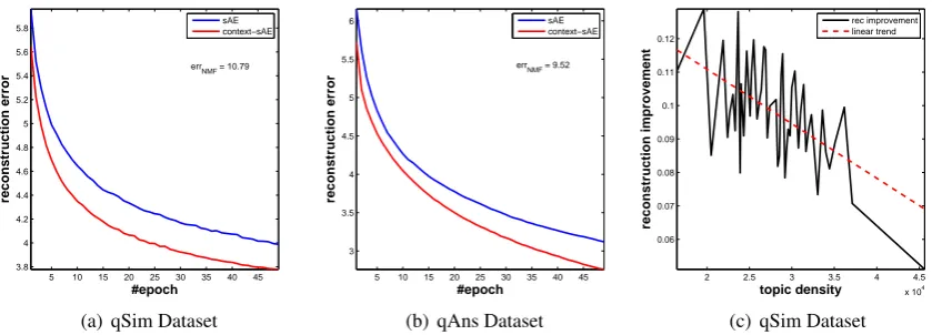
Figure 5: Reconstruction Error and Improvement: (a) and (b) reconstruction error on qSim and qAns respectively. errNMF shows the reconstruction error of NMF. Smaller error is better, (c) improvement
in reconstruction error vs. topic density: greater improvement is obtained in topics with lower density.
Model P@1 P@5 P@10
PCNN 20.0 33.8 40.4
SAE 16.8 29.4 32.8
CSAE 21.4 34.9 37.2
PBOW-PCNN 22.3 39.7 46.4
SAE-DST 22.2 35.9 42.0
[image:8.595.72.291.286.365.2]CSAE-DST 24.6 37.9 38.9
Table 6: Question ranking insupervisedsetting
Model P@1 P@5 P@10
SAE 17.3 32.4 32.8
CSAE 18.6 33.2 34.1
Table 7: Question ranking inunsupervisedsetting
5 Performance Analysis and Discussion We investigate the effect of context information in reconstructing inputs and try to understand rea-sons for improvement in reconstruction error. We compute the average reconstruction error of SAE and CSAE (Equations (3) and (7)). For these ex-periments, we setλ = 0 in Equation (7) so that we can directly compare the resulting loss of the two models. CSAE will still use context informa-tion withλ= 0but itdoes not backpropagate the reconstruction loss of context information.
Figures 5(a) and 5(b) show the average recon-struction error of SAE and CSAE on qSim and qAns datasets. Context information conistently improves reconstruction. The improvement is greater on qSim which contains smaller number of words per question as compared to qAns. Also, both models generate smaller reconstruction errors than NMF (Section 2.3). The lower performance of NMF is because it reconstructs inputs merely using global topics identified in datasets, while our
models utilize both local and global information to reconstruct inputs.
5.1 Analysis of Context information
The improvement in reconstruction error mainly stems from areas in data where “topic density” is lower. We define topic density for a topic as the number of documents that are assigned to the topic by our topic model. We compute the average im-provement in reconstruction error for each topicTj
using the loss functions for the basic and context-sensitive autoencoders:
∆j = |T1
j| X
x∈Tj
l(x)−l(x,hx)
where we setλ = 0. Figure 5(c) shows improve-ment of reconstruction error versus topic density on qSim. Lower topic densities have greater im-provement. This is because they have insufficient training data to train the networks. However, in-jecting context information improves the recon-struction power of our model by providing more information. The improvements in denser areas are smaller because neural networks can train ef-fectively in these areas.6
5.2 Effect of Depth
The intuition behind deep autoencoders (and, gen-erally, deep neural networks) is that each layer learns a more abstract representation of the in-put than the previous one (Hinton and Salakhut-dinov, 2006; Bengio et al., 2013). We investigate
1 2 3 4 5 6 7 60
62 64 66 68 70 72
#hidden layers
ρ
correlation
[image:9.595.112.251.71.188.2]Pe−trained CSAE−LC CSAE−LGC
Figure 6: Effect of depth in contextual word simi-larity. Three hidden layers is optimal for this task.
if adding depth to our context-sensitive autoen-coder will improve its performance in the contex-tual word similarity task.
Figure 6 shows that as we increase the depth of our autoencoders, their performances initially im-prove. The CSAE-LGC model that uses both lo-cal and global context benefits more from greater number of hidden layers than CSAE-LC that only uses local context. We attribute this to the use of global context in CSAE-LGC that leads to more accurate representations of words in their context. We also note that with just a single hidden layer, CSAE-LGC largely improves the performance as compared to CSAE-LC.
6 Related Work
Representation learning models have been ef-fective in many tasks such as language model-ing (Bengio et al., 2003; Mikolov et al., 2013b), topic modeling (Nguyen et al., 2015), paraphrase detection (Socher et al., 2011), and ranking tasks (Yih et al., 2013). We briefly review works that use context information for text representation.
Huang et al. (2012) presented an RNN model that uses document-level context information to construct more accurate word representations. In particular, given a sequence of words, the ap-proach uses other words in the document as exter-nal (global) knowledge to predict the next word in the sequence. Other approaches have also mod-eled context at the document level (Lin et al., 2015; Wang and Cho, 2015; Ji et al., 2016).
Ji et al. (2016) presented a context-sensitive RNN-based language model that integrates repre-sentations of previous sentences into the language model of the current sentence. They showed that this approach outperforms several RNN language models on a text coherence task.
Liu et al. (2015) proposed a context-sensitive RNN model that uses Latent Dirichlet Alloca-tion (Blei et al., 2003) to extract topic-specific word embeddings. Their best-performing model regards each topic that is associated to a word in a sentence as a pseudo word, learns topic and word embeddings, and then concatenates the embed-dings to obtain topic-specific word embedembed-dings.
Mikolov and Zweig (2012) extended a basic RNN language model (Mikolov et al., 2010) by an additional feature layer to integrate external in-formation (such as topic inin-formation) about inputs into the model. They showed that such informa-tion improves the perplexity of language models.
In contrast to previous research, we integrate context into deep autoencoders. To the best of our knowledge, this is the first work to do so. Also, in this paper, we depart from most previ-ous approaches by demonstrating the value of con-text information in sentence-level semantic simi-larity and ranking tasks such as QA ranking tasks. Our approach to the ranking problems, both for Answer Ranking and Question Ranking, is dif-ferent from previous approaches in the sense that we judge the relevance between inputs based on their context information. We showed that adding sentential or document context information about questions (or answers) leads to better rankings.
7 Conclusion and Future Work
We introduce an effective approach to integrate sentential or document context into deep autoen-coders and show that such integration is impor-tant in semantic similarity tasks. In the future, we aim to investigate other types of linguistic context (such as POS tag and word dependency informa-tion, word sense, and discourse relations) and de-velop a unified representation learning framework that integrates such linguistic context with repre-sentation learning models.
Acknowledgments
References
Yoshua Bengio, R´ejean Ducharme, Pascal Vincent, and Christian Janvin. 2003. A neural probabilistic
lan-guage model. J. Mach. Learn. Res., 3:1137–1155,
March.
Yoshua Bengio, Aaron Courville, and Pierre Vincent. 2013. Representation learning: A review and new
perspectives. Pattern Analysis and Machine
Intelli-gence, IEEE Transactions on, 35(8).
David M Blei, Andrew Y Ng, and Michael I Jordan.
2003. Latent dirichlet allocation. the Journal of
ma-chine Learning research, 3:993–1022.
Jordan L Boyd-Graber and David M Blei. 2009.
Syn-tactic topic models. InProceedings of NIPS.
Xinxiong Chen, Zhiyuan Liu, and Maosong Sun. 2014. A unified model for word sense representation and
disambiguation. InProceedings of EMNLP.
St´ephane Clinchant and Florent Perronnin. 2013. Ag-gregating continuous word embeddings for
informa-tion retrieval. the Workshop on Continuous Vector
Space Models and their Compositionality, ACL. Cicero Dos Santos, Luciano Barbosa, Dasha
Bog-danova, and Bianca Zadrozny. 2015. Learning hy-brid representations to retrieve semantically
equiva-lent questions. InProceedings of ACL-IJCNLP.
Michael Heilman and Noah A Smith. 2010. Tree edit models for recognizing textual entailments,
para-phrases, and answers to questions. InProceedings
of NAACL.
Geoffrey E Hinton and Ruslan R Salakhutdinov. 2006. Reducing the dimensionality of data with neural
net-works. Science, 313(5786):504–507.
Eric H Huang, Richard Socher, Christopher D Man-ning, and Andrew Y Ng. 2012. Improving word representations via global context and multiple word
prototypes. InProceedings of ACL.
Mohit Iyyer, Varun Manjunatha, Jordan Boyd-Graber, and Hal Daum´e III. 2015. Deep unordered compo-sition rivals syntactic methods for text classification. InProceedings of ACL-IJCNLP.
Yangfeng Ji, Trevor Cohn, Lingpeng Kong, Chris Dyer, and Jacob Eisenstein. 2016. Document context
lan-guage models. ICLR (Workshop track).
S. Kokoska and D. Zwillinger. 2000. CRC Standard
Probability and Statistics Tables and Formulae, Stu-dent Edition. Taylor & Francis.
Quoc V. Le and Tomas Mikolov. 2014. Distributed
representations of sentences and documents. In
Pro-ceedings of ICML.
Jiwei Li and Eduard Hovy. 2014. A model of coher-ence based on distributed sentcoher-ence representation. InProceedings of EMNLP.
Rui Lin, Shujie Liu, Muyun Yang, Mu Li, Ming Zhou, and Sheng Li. 2015. Hierarchical recurrent neural
network for document modeling. InProceedings of
EMNLP.
Chuan-bi Lin. 2007. Projected gradient methods for
nonnegative matrix factorization. Neural
computa-tion, 19(10):2756–2779.
Yang Liu, Zhiyuan Liu, Tat-Seng Chua, and Maosong
Sun. 2015. Topical word embeddings. In
Proceed-ings of AAAI.
Tomas Mikolov and Geoffrey Zweig. 2012. Context dependent recurrent neural network language model. InSpoken Language Technologies. IEEE.
Tomas Mikolov, Martin Karafiat, Lukas Burget, Jan Cernocky, and Sanjeev Khudanpur. 2010.
Recur-rent neural network based language model. In
Pro-ceedings of INTERSPEECH.
Tomas Mikolov, Kai Chen, Greg Corrado, and Jeffrey Dean. 2013a. Efficient estimation of word
represen-tations in vector space.arXiv:1301.3781.
Tomas Mikolov, Ilya Sutskever, Kai Chen, Greg S Cor-rado, and Jeff Dean. 2013b. Distributed representa-tions of words and phrases and their
compositional-ity. InProceedings of NIPS.
Arvind Neelakantan, Jeevan Shankar, Alexandre Pas-sos, and Andrew McCallum. 2014. Efficient non-parametric estimation of multiple embeddings per
word in vector space. InProceedings of the EMNLP.
Dat Quoc Nguyen, Richard Billingsley, Lan Du, and Mark Johnson. 2015. Improving topic models with
latent feature word representations. TACL, 3:299–
313.
Jeffrey Pennington, Richard Socher, and Christopher Manning. 2014. Glove: Global vectors for word
representation. InProceedings of EMNLP.
Sascha Rothe and Hinrich Sch¨utze. 2015. Autoex-tend: Extending word embeddings to embeddings
for synsets and lexemes. In Proceedings of
ACL-IJNLP.
Aliaksei Severyn and Alessandro Moschitti. 2013. Au-tomatic feature engineering for answer selection and
extraction. InProceedings of EMNLP.
Aliaksei Severyn and Alessandro Moschitti. 2015. Learning to rank short text pairs with convolutional
deep neural networks. InProceedings of SIGIR.
Carina Silberer and Mirella Lapata. 2014. Learn-ing grounded meanLearn-ing representations with
autoen-coders. InProceedings of ACL.
Richard Socher, Eric H. Huang, Jeffrey Pennington, Andrew Y. Ng, and Christopher D. Manning. 2011. Dynamic pooling and unfolding recursive
autoen-coders for paraphrase detection. InProceedings of
Keith Stevens, Philip Kegelmeyer, David Andrzejew-ski, and David Buttler. 2012. Exploring topic
co-herence over many models and many topics. In
Pro-ceedings of EMNLP-CNNL.
Pascal Vincent, Hugo Larochelle, Yoshua Bengio, and Pierre-Antoine Manzagol. 2008. Extracting and composing robust features with denoising
autoen-coders. InProceedings ICML.
Pascal Vincent, Hugo Larochelle, Isabelle Lajoie, Yoshua Bengio, and Pierre-Antoine Manzagol. 2010. Stacked denoising autoencoders: Learning useful representations in a deep network with a local
denoising criterion. The Journal of Machine
Learn-ing Research, 11:3371–3408.
Tian Wang and Kyunghyun Cho. 2015. Larger-context
language modelling. CoRR, abs/1511.03729.
Mengqiu Wang, Noah A. Smith, and Teruko Mita-mura. 2007. What is the Jeopardy model? a
quasi-synchronous grammar for QA. In Proceedings of
EMNLP-CoNLL.
Xuchen Yao, Benjamin Van Durme, Chris Callison-burch, and Peter Clark. 2013. Answer extraction
as sequence tagging with tree edit distance. In
Pro-ceedings of NAACL.
Wen-tau Yih, Ming-Wei Chang, Christopher Meek, and Andrzej Pastusiak. 2013. Question answering using
enhanced lexical semantic models. InProceedings
of ACL.
Lei Yu, Karl Moritz Hermann, Phil Blunsom, and Stephen Pulman. 2014. Deep learning for answer
sentence selection. InNIPS, Deep Learning
Work-shop.
Matthew D. Zeiler. 2012. ADADELTA: an adaptive