The Heterogeneity Among Commodity Rich Economies: Beyond the Prices of Commodities

Munich Personal RePEc Archive

The Heterogeneity Among

Commodity-Rich Economies: Beyond the

Prices of Commodities

Troug, Haytem

university of Exeter

14 February 2019

The Heterogeneity Among Commodity-Rich Economies:

Beyond the Prices of Commodities

Haytem Troug

March 8, 2019

Abstract

The existing literature has always assumed that commodity-rich countries are a

homoge-neous group, resulting in the generalisation of any findings obtained from a single

commodity-rich economy. This paper proposes a small open economy model for a commodity-commodity-rich country

and studies the triggers of business cycles for four different commodity-rich economies to

high-light the existence of heterogeneity among commodity-rich economies. The model introduces

government consumption in a non-separable form to the utility function. Commodities have a

central role in private consumption, production of final goods, and windfalls for the domestic

government. We feed the model with a variety of shocks that were previously proposed by the

previous literature. The estimations of the model show that oil-rich economies are more

vul-nerable to external shocks than their commodity-rich counterparts. This is mainly the result

of the size of commodity windfalls in the economy, as the share of oil revenues are significantly

higher than the revenues of other commodities, as a ratio of output. The results also show

that there exists a policy crowding out effect of fiscal policy to monetary policy in oil-rich

economies, all explaining the choice of an exchange rate peg regime in most oil-rich economies.

Keywords: New Keynesian models, Business Cycle, Open Economy Macroeconomics, Joint

Analysis of Fiscal and Monetary Policy, Commodity Prices.

JEL classification: E12, E32, E63, F41.

1

Introduction

There exists a long and growing literature that investigates the effect of commodities on

commodity-rich economies. The seminal paper by Sachs and Warner 1995 illustrated the adverse effect of the abundance of natural resources on economic growth. In addition,Ploeg and Poelhekke 2009

illustrate that the high volatility of commodity prices seems to be the quintessence of the resource

curse since it generates large real exchange rate fluctuations and less investment, especially in

countries where financial development is lagging (Aghion et al. 2009). Nevertheless, the above findings were challenged by numerous papers that have questioned the natural resource curse,

pointing to examples of commodity-exporting countries that have done well, such as Chile, Norway

and Botswana1_{. Moreover, Alexeev and Conrad 2009, Cotet and Tsui 2010and Havranek et al.} 2016find very little evidence in support of the natural resource curse, while Ploeg 2011 showed empirical evidence that either outcome is possible, leading the literature to deviate from consensus

on this issue. Another seminal paper byMehlum et al. 2006 showed that institutions are a vital factor for the effect of resources on economic performance2_.

One possible explanation for the above disparity is that the literature mentioned above usually

assumes that this group of countries is homogeneous. For instance, many studies that have been

conducted on a single rich economy assumed that their results apply on all

commodity-rich economies, labelling their case study as "prototypical" or "quintessential"3_{. In this paper, we}

try to contribute to the growing literature on natural resources and economic performance by

highlighting one possible source of heterogeneity among commodity-rich economies. We try to

capture this heterogeneity by imposing the same commodity-price shock on a number of

resource-rich economies. Doing so will allow us to show how the social capabilities of each economy and

the characteristics of the commodity affect the response of key macroeconomic variables to a

commodity-price shock. Two findings in the literature motivate our approach. The first isRodrik 1999’s findings that the magnitude of a country’s growth deceleration since the 1970’s is a function 1_{Larsen 2006exhibited Norway as an example of an oil-rich country that was able to escape the Resource Curse.}

Englebert 2000,Sarraf and Jiwanji 2001,Acemoglu et al. 2003andIimi 2006are among those noting Botswana’s conspicuous escape from the Resource Curse.

2_{These findings refute the findings ofSachs and Warner 1995of an insignificant role for institutions in overcoming} the resource curse, and they show that the quality of institutions has to increase as the size of resources increase in the economy.

of both the magnitude of the shocks and a country’s social capability for adapting to shocks. Also,

Fernández et al. 2018findings that there is strong comovement among the prices of commodities. Thus, this will enable us to isolate the two factors affecting the response of macroeconomic variables

in each economy, and solely concentrate on the social capabilities and the characteristics of the

commodity. To the extent of our knowledge, the existing literature has not yet addressed this

phenomenon.

This paper proposes a small open economy model for a commodity-rich country to

quanti-tatively study the triggers of business cycles in different commodity-rich economies. This paper

extends the model used in Troug 2019 by adding some features to the model to make it more relevant for a commodity-rich economy. The model contains four key features. First, the supply

of commodities is exogenous, and it is affected by political, geographical, and technical factors,

i.e., non-economic factors. Second, the government is the sole owner of commodities and it

col-lects the windfalls of selling them to the rest of the world4_{. Third, the small open economy is a}

price taker for all goods and services it produces and consumes. Also, the small open economy is

affected by the second second-round effect of an increase in the commodity prices in the form of

high foreign inflation and low world demand. Fourth, households and firms, both in the domestic

economy and the rest of the world economy, use commodities for consumption and as a factor

of production, respectively. In addition, the main behavioural parameters that the paper focuses

on are the elasticity of substitution between government consumption and private consumption

and the response of government consumption to fluctuations in the commodity prices. The former

parameter is an indicator of the efficiency of government consumption and its effect on private

consumption (crowding-in versus crowding-out), while the latter captures the behaviour and the

stance of fiscal policy during booms and busts of commodity prices, along with the size of the

commodity windfalls in the government’s revenue.

The analysis of this paper proceeds in four steps. First, we empirically estimate our behavioural

parameters. Second, we generate the impulse response of the data using a structural VAR model.

Third, we illustrate the full structure of our DSGE model. The model generates extra sources of

stochastic processes that were proposed by the existing literature. The calibration of the parameters

4_{Introducing the fiscal sector was neglected byFernández et al. 2018, leaving out the most significant transmission} channel for commodities-price shocks in commodity-rich economies, as highlighted byCespedes and Velasco 2014

for our DSGE model is made for all of our economies of interest based on the empirical findings

of this paper and the long-term averages found in the data. Fourth, we use Bayesian estimation

techniques to calculate the variance decomposition of our variables of interest. The empirical and

theoretical findings of this paper show that consumption is excessively volatile relative to output,

which is consistent with the findings of the previous literature5_{. However, our findings show that}

this might also be the case for developed countries which are rich with natural resources, as in

the case of Australia. The results also show that, once we control for the commodity prices, there

is heterogeneity in the forces driving the business cycle within commodity-rich economies. The

fiscal sectors in these economies drive these forces, along with institutional factors and the share

of commodity windfalls in the government’s total revenue.

Our results show the existence of a procyclical fiscal stance in developing, commodity-rich

countries. This is consistent with the findings ofKaminsky et al. 2005,Frankel 2011, andBastourre et al. 2012. Nevertheless, we find that adopting the fiscal rule, as in the case of Chile and Australia, reverses this behaviour, consistent with the findings ofCespedes and Velasco 2014. Our findings also support the findings ofRodrik 1999andIsham et al. 2005of how the abundance of commodities erodes institutions, and that, in return, will affect how economies react to commodity shocks. The

results of this paper, at least regarding commodity-rich economies, strongly support the findings

of Gali et al. 2007and Bouakez and Rebei 2007 who show that government consumption has a crowding in effect on private consumption.

The paper also shows significant heterogeneity in the contribution of terms of trade to business

cycles among commodity-rich economies and illustrate that oil-rich economies are more vulnerable

to these shocks. These results complement the work of Fernández et al. 2018, Shousha 2016,

Fernández Martin et al. 2017, andDrechsel and Tenreyro 2017, who show a significant role for the proxy of terms of trade (commodity prices) in driving business cycles in developing economies6_{. The}

results of the paper show that the effect of external shocks on commodity-rich economies is sensitive

to the degree of openness in these economies and the adopted fiscal regime in each economy. This

is attributed to the fact that the government is the main channel for the transmission of these

5_{See, for example,Neumeyer and Perri 2005,Aguiar and Gopinath 2007,Garcia-Cicco et al. 2010,Akinci 2014,} andDrechsel and Tenreyro 2017.

fluctuations in commodity-rich economies as illustrated by Arezki and Ismail 2013. Our results also show that oil-rich countries, in this case as well, are more affected by external shocks than

their commodity-rich counterparts.

The organisation of the remainder of this paper is as follows. In the second chapter, we illustrate

our stylized facts and empirical findings for our economies of interest. In the third chapter, we

build a DSGE model for a commodity-rich small open economy. We add some structural shocks

that were suggested by the previous literature and calibrate the model based on our empirical

findings and the long-term parameters found in the data. In the fourth chapter, we estimate the

model using Bayesian estimation techniques. Chapter five concludes.

2

Stylized Facts

2.1

Data

Figure 1: Real GDP Growth and Commodities Prices

(a) Real GDP per Capita Growth (b) Commodities Prices

This paper uses real government consumption, real private consumption, and inflation for a selected

number of commodity-rich economies7 8_{. In addition to this, we add the same variables for the}

U.S economy, as it will be used to calibrate the moments of the rest of the world, as shown below.

7_{The selected countries are Chile, a Copper-rich economy; Australia, a minerals-rich economy; Saudi Arabia, an} oil-rich economy; and South Africa a coal and minerals-rich economy.

The source of this data is World Bank’s World Development Indicators (WDI) database, and all

of the series are presented in annual per capita terms.

The commodity prices indices were retrieved from the World Bank commodity prices database

(the pink sheet). All commodity prices were deflated using the U.S. CPI index. The deflation is

done to reflect the real purchasing power of commodity windfalls. We also use mean deviation of

real commodity prices rather than de-trending the series in order to capture long persistence in

commodity prices (super cycles). The data for the supply of commodities was downloaded from

the IEA database.

The above graph shows significant heterogeneity in the growth rate of GDP per capita among

the selected commodity-rich economies. We also include the US growth rate for reference. The

above figure illustrates how the growth rates of commodity-rich economies deviate from the growth

rate of GDP per capita in the US by different magnitudes. One possible explanation for this

behaviour is the volatility of the prices of commodities in these economies9_{, as shown in panel (b)}

of the above figure.

The above graph also shows comovement in the prices of commodities, consistent with the

findings ofFernández et al. 2018. As noted, the fluctuation of commodities prices results in high volatility in commodity-rich economies. In this paper, we impose the same commodity price on all

of our selected economies to capture the heterogeneity among these economies beyond the different

price fluctuations of each commodity. The price index that we impose in this paper is an average

of both the energy and non-energy indices. The energy price index is a weighted average of crude

oil prices, natural gas prices, and coal prices. Agricultural products and metal, on the other hand,

represent almost 97 % of the non-energy price index.

2.2

What Affects Commodity Prices?

The framework of the theoretical model assumes that commodity prices are determined by

com-modity supply10_{, World output, World technology, and World government consumption. Therefore,}

the analysis of this section will not affect the structure nor the design of this model, as the

pa-rameters that govern the effect of our independent variables on real commodity prices are derived

9_{See, for example,Rodrik 1999.}

endogenously in the model and not estimated. Nevertheless, this exercise is useful as it will give

us an indication of how real commodity prices are affected by developments in the macro variables

of the world economy. The regression of this section is specified in the following from:

˜

P_O,t∗ =β0+β1Yt∗+β2G∗t+β3Ot∗s+ǫt (1)

Where ˜P∗

O,t =

PO,t−_PO¯ ¯

PO ∗100 is the mean deviation of real commodity prices. Y

∗

t , G∗t, Ot∗s are world output, world government consumption and the supply of commodities, respectively.

The results of the regression are shown in the below table and they highlight a significant effect

of the supply of commodities and world output on real commodity prices. World government

consumption, however, does not significantly affect commodity prices. The signs of the effect of

the supply of commodities and world output are in line with the derivations of the DSGE model

of this paper, as shown below.

Table 1: Regression Results for Commodity Prices

Commodity Prices

World Output 1.46**

(0.566) World Government Consumption -1.046

(1.434) Commodities Supply -7.787***

(2.753)

Constant -614.7

(800.355)

Observations 36

R-squared 0.38

Standard errors in parentheses *** p <0.01, ** p <0.05, * p <0.1

2.3

In this section, we empirically estimate the effect of government consumption on private

con-sumption in the four commodity-rich economies and the U.S. economy, which represents the world

economy in this model. For the U.S. economy, we estimate the effect of government consumption

on private consumption, controlling for the commodity price index, U.S. output, and U.S. inflation.

inflation, and domestic output. The regression of this section is specified in the following from:

ln(Ct) =β0+χln(Gt) +β1ln(Xt) +ǫt (2)

WhereCt is private consumption, Gt is government consumption, and Xt is a vector of control

variables including world output, domestic output, domestic inflation and the real price of

com-modities. All variables are expressed in log forms. The key parameter of interest in this regression

isχ, which denotes the effect of government consumption on private consumption. The results of

the regressions show a significant positive effect of government consumption on private

consump-tion for all five economies. As these results represent one of our behavioural parameters, we will

use the below results in the baseline calibration part of our DSGE model, and they will be included

as priors in the Bayesian estimation.

Table 2: Regression Results for the Effect ofGonC

Domestic Consumption USA KSA CHL SA AUS

World Output 1.151*** -0.701*** -0.378** -0.037 0.781***

(0.016) (0.162) (0.175) (0.027) (0.177) World Government Consumption 0.056

(0.038)

World Inflation -0.524***

(0.143)

Domestic Output -0.073 1.119*** 1.127*** -0.624***

(0.202) (0.114) (0.106) (0.176)

Domestic Government Consumption 0.736*** 0.221* 0.145** 0.712***

(0.170) (0.121) (0.062) (0.135)

Domestic Inflation 0.642 -0.01 -0.074 -0.34

(1.63) (0.205) (0.276) (0.369)

Commodity Prices 0.035*** 0.177 -0.053 -0.022 0.038*

(0.005) (12.45) (0.04) (0.027) (0.02)

Constant -250.58*** 1116.506*** -138.52 -283.99*** 172.256**

(23.47) (358.63) (125.65) (93.027) (68.047)

Observations 36 36 36 36 36

R-squared 0.99 0.82 0.99 0.97 0.92

Bootstrap standard errors with 10,000 replications are in parentheses. *** p <0.01, ** p <0.05, * p <0.1.

The below results also contribute to the divided literature on the effect of government

con-sumption on private concon-sumption11_{. Our results support the literature that shows government}

consumption as a complement to private consumption, at least in commodity-rich countries.

Nev-ertheless, some of causality tests for all the regressions in this section show conflicting signs of

11_{Coenen et al. 2013,Gali et al. 2007, and Fiorito and Kollintzas 2004find that government consumption has}

the directions imposed by the regression assumptions. Also, we acknowledge the possibility of the

presence of endogeneity in the estimations. However, using a DSGE model in the next section will

allow us to overcome these problems, because it takes into account the fact that these variables are

simultaneously determined. Moreover, We will also further investigate this issue in the Bayesian

estimation section and, as shown below, the Bayesian estimations show that the explanatory power

of the data overcomes the prior values that we extract from the regression results in this section.

2.4

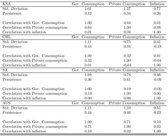
Business Cycle Moments

Table 3: Business Cycle Moments for Selected Economies

World GDP growth Gov. Growth Cons. Growth Inflation Mean 1.68 0.57 2.01 2.03 Std. Deviation 1.86 1.68 1.74 0.86 Persistence 0.32 0.59 0.50 0.33 Correlation with GDP growth 1.00 -0.04 0.94 -0.04 Correlation with Gov. Growth -0.04 1.00 0.06 -0.23 Correlation with Cons. Growth 0.94 0.06 1.00 -0.14 Correlation with inflation -0.04 -0.23 -0.14 1.00 KSA GDP growth Gov. Growth Cons. Growth Inflation Mean -1.51 2.40 1.47 1.35 Std. Deviation 8.75 10.02 9.21 2.33 Persistence 0.31 0.12 0.36 0.72 Correlation with GDP growth 1.00 -0.05 -0.14 0.28 Correlation with Cons. Growth -0.05 1.00 0.40 0.30 Correlation with Gov. Growth -0.14 0.40 1.00 0.45 Correlation with inflation 0.28 0.30 0.45 1.00 CHL GDP growth Gov. Growth Cons. Growth Inflation Mean 2.99 1.70 3.37 9.98 Std. Deviation 4.32 2.86 6.01 8.59 Persistence 0.25 0.44 -0.41 0.79 Correlation with GDP growth 1.00 0.35 0.92 -0.02 Correlation with Gov. Growth 0.35 1.00 0.25 -0.65 Correlation with Cons. Growth 0.92 0.25 1.00 -0.01 Correlation with inflation -0.02 -0.65 -0.01 1.00 SA GDP growth Gov. Growth Cons. Growth Inflation Mean 0.41 0.96 0.62 3.55 Std. Deviation 2.45 2.56 3.99 1.94 Persistence 0.43 0.35 0.03 0.77 Correlation with GDP growth 1.00 0.32 0.86 0.10 Correlation with Gov. Growth 0.32 1.00 0.26 0.14 Correlation with Cons. Growth 0.86 0.26 1.00 -0.03 Correlation with inflation 0.10 0.14 -0.03 1.00 AUS GDP growth Gov. Growth Cons. Growth Inflation Mean 1.75 0.38 0.38 2.42 Std. Deviation 1.66 1.22 1.85 1.04 Persistence 0.21 0.58 0.02 0.42 Correlation with GDP growth 1.00 -0.03 -0.40 -0.37 Correlation with Gov. Growth -0.03 1.00 0.19 -0.43 Correlation with Cons. Growth -0.40 0.19 1.00 0.15 Correlation with inflation -0.37 -0.43 0.15 1.00

The above table shows that private consumption in developing countries fluctuates more than

consumption fluctuates more than output, highlighting the possibility of commodities affecting the

business cycle of developed economies the same way they affect developing economies. The above

persistence measures were estimated by fitting an AR(1) model for each variable.

The above table also shows that the behaviour of the growth rates of per capita government

consumption demonstrates significant differences among the above economies. This variable shows

more volatility in Saudi Arabia (an oil-rich economy). The growth rates of the same variable for

South Africa and Chile, although three times less volatile than that of the Saudi economy, are still

higher than the volatility of government consumption in the U.S. economy. Conversely, the growth

of government consumption in Australia, which is a developed economy, showed less volatility than

all of the above countries, including the U.S. Furthermore, the volatility in government consumption

is positively correlated with the volatility of output per capita and the persistence of the growth

of government consumption is negatively correlated with its volatility across all economies. These

indicators demonstrate the different degrees of volatility among commodity-rich economies which

might result from different factors that we aim to study in this paper we remove the effect of

commodity prices.

2.5

The Reaction of Government Consumption to Changes in

Commod-ity Prices

In this section, we estimate the second and probably most important behavioural parameter in

the model. We empirically estimate the reaction of government consumption in our selected four

economies to changes in the average commodity index. The magnitude of the response of

govern-ment consumption to changes in commodity prices will be an indicator of two important factors.

The first is the fiscal disciplines of the domestic government while the second is the size of the

resource rent in the economy. We control for domestic output and domestic CPI inflation. The

regression of this section is specified in the following from:

ln(Gt) =β0+φgp˜∗O,t+β1ln(Xt) +ǫt (3)

variables are expressed in log forms. As noted above, the key parameter of interest in this

regres-sion isφg, which denotes the response of government consumption to changes in real commodity

prices.

Table 4: Regression Results for the reaction of G to changes in Commodity prices

Government Consumption KSA CHL SA AUS

Commodity Prices 0.78*** 0.25*** -0.04 -0.01

(0.14) (0.048) (0.08) (0.017)

Domestic Output -0.713 0.44*** 0.87*** 0.29***

(2.27) (0.10) (0.26) (0.025)

Domestic Inflation -0.212 0.11 2.24 -0.9*

(0.375) (0.314) (0.59) (0.48)

Constant 1161.3*** 637.95*** -33.16 475.7***

(418.13) (162.69) (278.30) (26.9)

Observations 36 36 36 36

R-squared 0.63 0.94 0.77 0.83

Bootstrap standard errors with 10,000 replications are in parentheses. *** p <0.01, ** p <0.05, * p <0.1.

The above results show that the reactions of the domestic governments display considerable

dif-ferences among commodity-rich economies. While government consumption does not significantly

react to changes in the prices of commodities in Australia and South Africa, it was significantly

positive in Chile and Saudi Arabia with responses of differing degrees. The response of government

consumption in Saudi Arabia is three times the response of government consumption in Chile. One

possible explanation for this behaviour is the size of the resource rents in the economy. During our

estimation period, resource rents as a percentage of GDP in Saudi Arabia, Chile, South Africa, and

Australia averaged 34 %, 10.9 %, 6.25 % and 4.8 %, respectively (as shown inAppendix C.3)12_.

The above estimations of this behavioural parameter will also be used below in the baseline

calibration of our model. These values will also be used as priors in the Bayesian estimation to be

undertaken later.

2.6

Structural VAR Model

In this section, we address the effect of a commodity shock on the domestic economy by providing

an empirical measure based on a Structural VAR model. Commodity shocks are easier to

cap-ture as they are observed, different from unobserved technology shocks. Thus, understanding the

12_{InAppendix C.3we report the resource rents averages for 88 countries. The stark finding in the data is the}

channels by which the effect of commodity prices affects economic activity is crucial from a policy

perspective.

The Structural VAR model for each domestic economy includes four variables, namely the real

commodity price index, the growth rate of real government consumption per capita, the growth

rate of real private consumption per capita, and domestic CPI inflation, using annual data over

the period 1980 to 2015 and defined as follows:

A0Yt=αt+A1Yt−1+...+ApYt−p+ut (4)

Yt is a vector containing the four variables of interest for each economy. The underlying

assumption that we make for this Structural VAR model is that real commodity prices are not

contemporaneously affected by developments in the domestic economies. This is consistent with

the small open economy framework that we adopt in this paper. Thus, having commodity prices

first in the order of our variables in a Cholesky decomposition is a plausible assumption. The

second variable in order is the growth rate of government consumption. This ordering is in line

withPieschacon 2012, Gali et al. 2007and Fatas and Mihov 2001. It is also consistent with the analysis of this paper in showing how commodity shocks are transmitted to the economy through

the fiscal sector. The results below are robust to different ordering between private consumption

and inflation. In addition, the optimal lag criteria suggests that a lag of order 1 is the optimal

choice for each of the four economies.

The economic principle behind the effect of a commodity price shock in our model is simple.

When positive, a commodity-price shock acts as an income shock that increases government

con-sumption. In return, The increase in government consumption will boost private consumption and

put inflationary pressure on domestic prices, if government consumption has a crowding in effect

Figure 2: Response to a Commodity Shock

The impulse responses illustrate how government consumption growth responds in a different

manner among commodity-rich economies. The response of government consumption in Saudi

Arabia, an oil-rich country, is the highest among its counterparts in this study. In addition, the

insignificant response of Australia and Chile reflect the adopted fiscal policy objective or rule in

these two economies. The reaction of the South African government consumption shows a positive

reaction to a commodity-price shock. This contradicts with the findings of the previous estimations

of this paper. Nevertheless, the Bayesian estimation section should confirm one of these findings.

The reaction of private consumption and domestic CPI inflation is determined by the crowding

in effect of government consumption and the implemented subsidies schemes that are adopted in

different commodity-rich economies. In this regard, the size of the consumption of commodities

in the aggregate consumption bundle should reflect the size of these subsidies in our DSGE model

below.

The next section builds a dynamic general equilibrium model guided by these stylized facts

into fluctuations in real economic activity, along with other exogenous shocks that have been

suggested by the previous literature.

3

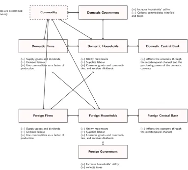
The Model

Domestic Households Domestic Government Commodity

Domestic Firms Domestic Central Bank

Foreign Households

Foreign Firms Foreign Central Bank

Foreign Government (+) Utility maximisers (+) Supplies labour

(+) Consume goods and commodi-ties, and receives dividends

(+) Utility maximisers (+) Supplies labour

(+) Consume goods and commodi-ties, and receives dividends (+) Supply goods and dividends

(+) Demand labour

(+) Use commodities as a factor of production

(+) Supply goods and dividends (+) Demand labour

(+) Use commodities as a factor of production

(+) Increase households’ utility (+) Collects commodities windfalls and taxes

(+) Increase households’ utility (+) collects taxes

(+) Affects the economy through the intertemporal channel and the purchasing power of the domestic currency

(+) Affects the economy through the intertemporal channel (+)Prices are determined

endogenously

Figure 3: Structure of the Model

In this section we construct a small open economy model for a commodity-rich economy by using

the framework of Galí and Monacelli 2005. Moreover, we extend the model used in Troug 2019

by adding some features that were missing in the model to make it relevant for a commodity-rich

economy. Our model allows for a quadruple role for commodities. First, the domestic government

collects the windfalls from selling commodities to the rest of the world. Second, commodities are

both in the domestic economy and the foreign economy use commodities as an input factor in their

production. Lastly, the domestic economy is affected by the second-round effect of an increase in

commodity prices in the form of high foreign inflation and low world demand or vice versa.

3.1

Domestic Economy

3.1.1 Household

The representative consumer in the domestic economy seeks to maximise the following discounted

lifetime utility function:

E0

∞

X

t=0

βtU( ¯Ct, Nt) (5)

The utility function is assumed to be continuous and twice differentiable. Nt is the number

of hours worked; β is the discount factor; ¯Ct is the aggregate consumption bundle. The

aggre-gate consumption bundle is a constant elasticity of substitution aggreaggre-gate that consists of private

consumptionCt and government consumptionGt:

¯

Ct=

h

δχCt1−χ+ (1−δ)χG

1−χ t

i1−1χ

(6)

Whereδis the equilibrium share of private consumption in the aggregate consumption bundle

andχ is the inverse elasticity of substitution between private consumption and government

con-sumption. From equations (5) and (6) we can notice that the utility function is non-decreasing in government consumption Gt. The above utility function is subject to the following budget

constraint:

Z 1

0

PH,t(j)CHt(j)dj+

Z 1

0

Z 1

0

Pi,t(j)Cit(j)djdi+EtQt,t+1Dt+1≤Dt+WtNt+Tt (7)

WhereDtis the nominal payoff for bonds, shares in firms and deposits held at the end of period

t and mature at period t+1. Qt,t+1 is a stochastic discount factor of nominal payoffs and it is

equal to _Rt1; Wt is wages;Tt is lump-sum transfers to the households net of lump-sum taxes. All

a composite of core consumption and consumption of commodities:

Ct=

h

(1−̟)1µ_C µ−1

µ Z,t +̟

1 µ_C

µ−1 µ O,t

iµµ−1

(8)

In the above equation,CO,t is consumption of commodities by the domestic economy’s households,

and̟ is the share of commodities consumption in the household’s consumption bundle. CZ,t is

the non-commodity consumption bundle (core consumption), and it has a size of (1−̟) in the

household’s consumption bundle. µis the elasticity of substitution between core consumption and

consumption of commodities. The core consumption bundleCZ,t is a CES composite of home and

foreign goods defined as follows:

CZ,t=

h

(1−α)1η_C η−1

η H,t + (α)

1 η_C

η−1 η F,t

iη−η1

(9)

The above equation is the same household’s consumption bundle used byGalí and Monacelli 2005, which is the workhorse for small open economies. αhere is the degree of openness in the economy which represents the share of imported goodsCF,tin the household’s consumption bundle.

The home bias parameter (1−α) produces the possibility of a different consumption bundle in

each economy. This is a consequence of having different consumption baskets in each country,

despite the law of one price holding for each individual good. η >0 is the elasticity of substitution

between domestically produced goods and imported goods in the household’s consumption bundle.

The above utility function assumes two separabilities. The first is the separation between

consumption and the amount of hours worked, and the second is time separability. The household’s

problem is analysed in two stages here. We first deal with the expenditure minimisation problem

faced by the representative household to derive the demand functions for commodity goods,

non-commodity goods, domestic goods and foreign goods. In the second stage, the households choose

the level ofCtandNt, given the optimally chosen combination of goods. The standard optimality

condition for households will be as follows:

Wt

Pt

=N_tϕC¯_tσC_¯t Ct

χ

The intertemporal optimality condition is:

βC¯t_¯+1 Ct

χ−σ P_t

Pt+1

C_t

Ct+1

χ

=Qt,t+1 (11)

Taking the conditional expectation of equation (11) and rearranging the terms we get:

βRtEt

hC¯_t+1

¯

Ct

χ−σ P_t

Pt+1

C_t

Ct+1

χi

= 1 (12)

3.2

Firms

3.2.1 Price Setting Behaviour

The firms in this model set their prices in a staggered manner following Calvo 198313_{. Under}

Calvo contracts, we have a random fraction 1−θ of firms that are able to reset their prices at

periodt, while prices of the remaining firms of sizeθare fixed at the previous period’s price levels.

Therefore, we can say thatθk _{is the probability that a price set at period t will still be valid at}

periodt+k. Also, the probability of the firm re-optimising its prices will be independent of the

time passed since it last re-optimised its prices, and the average duration for prices not to change

is ₁₋1_θ. Given the above information, the aggregate domestic price level will have the following form:

PH,t=

h

θ(PH,t−1)1−ǫ+ (1−θ)( ¯P_H,t1−ǫ)

i1−1ǫ

(13)

Where ¯PH,t is the new price set by the optimising firms. From the derivations shown in

Appendix C.2, we get the following form for inflation:

Π1−ǫ

H,t =θ+ (1−θ)

P¯_H,t

Pt−1

1−ǫ

(14)

The above equation shows that the domestic inflation rate at any given period will be solely

determined by the fraction of firms that reset their prices at that period. When a given firm in the

economy sets its prices, it seeks to maximise the expected discounted value of its stream of profits,

13_{The Calvo model makes aggregation easier because it gets rid of the heterogeneity in the economy. The}

conditional that the price it sets remains effective:

max_PH,t¯

∞

X

k=0

θkEtQt,t+k[cjt+k|t( ¯PH,t−Ψt+k)] (15)

The above equation is subject to a sequence of demand constraints: cjt+k =

_PH,t¯

PH,t+k

−ǫ

Ct.

Solving this problem (also shown inAppendix C.2) yields the following optimal decision rule:

∞

X

k=0 θkEt

n

Qt,t+kCt+k

h P¯_H,t

PH,t−1

− MM Ct+k|tΠHt−1,t+k

io

= 0 (16)

WhereMis the firm’s markup at the steady state andM Ctis real marginal cost. As we can see

from equation (16), in the sticky price scheme producers, given their forward-looking behaviour, adjust their prices at a random period to maximise the expected discounted value of their profits

at that period and in the future. Thus, firms in this model will set their prices equal to a markup

plus the present value of the future expected stream of their marginal costs. This is done because

firms know that the price they set at periodtwill remain effective for a random period of time in

the future. We also assume that all firms in the economy face the same marginal cost, given the

constant return to scale assumption imposed on the model and the subsidy that the government

pays to firms, as we will see in the following section. The firms also use the same discount factor

β as the one used by households, and this is attributed to the fact that the households are the

shareholders of these firms. Additionally, all the firms that optimise their prices in any given period

will choose the same price which is also a consequence of the firms facing the same marginal cost.

Equation (16) also shows that the inflation rate is proportional to the discounted sum of the future real marginal costs additional to a mark-up resulting from the monopolistic power of the firms.

3.2.2 Production

Firm (j) in the domestic economy produces a differentiated good following a linear production

function:

Yt(j) = [AtNt(j)]νOtd(j)

1−ν ₍₁₇₎

of technology in the production function. It evolves exogenously and is assumed to be common

across all firms in the economy.Nt(j) is the labour force employed by firm (j). O_tdis the commodity

used in the production process and (1−ν) is the size of commodities in the production function.

The log form of total factor productivity at = log(At) is assumed to follow an AR(1) process:

at=ρaat−1+ǫa,t. Whereρa is the autocorrelation of the shock and the innovation to technology

ǫa,tis assumed to have a zero mean and a finite varianceσa. The cost minimisation function for

firm (j) has the following form:

(1−τ)(1−ν)WtNt(j) =νPo,tOdt(j) (18)

We note that in the above equation we left Wt without any firm specification, as we have a

competitive labour market in this model. Also, τ is the subsidy that the government gives to

firms in order to eliminate the markup distortion created by the firms’ monopolistic power. The

marginal cost equation takes the following form:

M Ct(j) = (1−τ)Wt

νAν

tOtd(j)1−νNt(j)ν−1

(19)

Using the above cost minimising equation, the above marginal cost equation is utilised to:

M Ct(j) = (1−τ) ν_Wν

tPo,t1−ν

νν_(1−ν)(1−ν)_Aν t

(20)

Lastly, given that aggregate output and aggregate employment in the domestic economy are

defined by theDixit and Stiglitz 1977aggregator, the aggregate production function will take the following form:

Yt= [AtNt]νOd

(1−ν)

t (21)

3.3

Fiscal Policy

The government levies a lump sum tax on households and pays a subsidy to firms in order to

eliminate its monopolistic power. The government also collects windfalls from sales of its natural

defined as14_:

Gt+ (1 +Rt−1)Bt−1+τ =Bt+Tt+φgPt,oYt,o (22)

WhereBt is the quantity of a riskless one-period bond maturing in the current period, which

pays one unit. Rtdenotes the gross nominal return on bonds purchased in period t. The

govern-ment levies a non-distortionary lump-sum taxTt to finance its consumption and pay a subsidyτ

to firms. In addition, po

t is the price of commodities dominated in domestic currency and Yto is

the output of that commodity15_{. Given the above, G}

t is government consumption will take the

following form:

Gt

G =

nG_t−1

G

oρgnP_o,tY_o

PoYo

oφg

exp(ζG,t) (23)

Where 0 < ρg < 1 is the autocorrelation of government consumption, and it captures the

persistence of government consumption. φg captures the response of government consumption to

changes in the prices of commodities. ζG,t represents an i.i.d. government spending shock with

constant varianceσ2

g.

3.3.1 Monetary Policy

The monetary authorities in this model use a short-term interest rate as their policy tool. In

this case, we have a cashless economy where money supply is implicitly determined to achieve the

interest rate target. It is also assumed that the central bank will meet all the money demanded

under the policy rate it sets.

Rt

R =

nΠZ,t

ΠZ

oφπnY_t

Y

oφx

exp(ζR,t) (24)

The parameters of the above equations (φπ, φx) describe the strength of the response of the

policy rate to deviations in the variables on the right-hand side. These parameters are assumed

14_{The definition of government consumption includes all government recurrent spending items. We do this to}

establish consistency in the mapping between the model’s government consumption variable and the observed government consumption variable.

15_{Given the fact that the production of natural resources is capital intensive, we follow the existing literature}

to be non-negative. The inflation response parameterφπ in the above policy rule must be strictly

greater than one in order for the solution of the model to be unique, as shown byBullard and Mitra 2002. Lastly, ζR,t represents an i.i.d. monetary policy shock with constant varianceσR2.

3.4

International Linkages

We first start by the defining the terms of trade as the ratio of imported prices to domestic

prices. The bilateral terms of trade index between the domestic economy and any other small

economy (country i) is defined as: Si,t = _PH,tPi,t. The aggregate terms of trade index is defined

as: St=

R1

0 S 1−γ i,t di

1−1γ

. Defining PF,t =

R1

0 P 1−γ i,t di

1−1γ

allows as us to define the aggregate

effective terms of trade as:

St=

PF,t

PH,t

(25)

If we plug in the log-linearised representation of the imported prices index from the above

equation (pF,t=st+pH,t) in the log-linearised form of the CPI price index equation, we can derive

the CPI index as a function of the domestic prices index and the terms of trade:

pt=pH,t+αst (26)

The above function shows that the gap between the CPI index and the domestic price index

is filled by the terms of trade, representing imported inflation. This gap is parametrised by the

degree of openness of the domestic economy. Before progressing on further derivations, we first

define the bilateral exchange rateE_i,tas the value of country i’s currency in terms of the domestic

currency. Assuming that the law of one price holds, the price of any good in country (i) will be

equal to:

Pi,t(j) =Ei,tPi,ti (j) (27)

Integrating the above equation yields the price index for country (i). Solving this integral for

the imported prices index in the domestic economy yields:

The nominal effective exchange rate is equal to Et ≡ R

1

0 Ei,tdi, and the world price index

is defined as P_t∗ ≡ R1

0 Pi,tdi. Plugging the value of the imported prices index from the above

equation in the definition of the terms of trade yields:

St=

EtPt∗

PH,t

(29)

We now define the bilateral real exchange rate as the ratio of the price index in country (i)

to the CPI index in the domestic economy: REERi,t =

Ei,tPi t

Pt . Integrating the bilateral real

exchange rate equation yields the real effective exchange rate equation for the domestic economy:

REERt = EtP

∗

t

Pt . From the definitions of the terms of trade and the real effective exchange rate,

we can define the equation that links the two variables in a log-linearised form as follows:

qt= (1−α)st (30)

Under the assumption of complete international financial markets, the price of a one-period

riskless bond dominated in the domestic economy’s currency from country (i) is equal to: Ei,tQit=

E[E_i,t+1Qt,t+1]. If we add this equation to the domestic bond’s price equation (Qt=E[Qt,t+1]),

we get the uncovered interest parity condition:

Qi t

Qt =Et

E_i,t+1

E_i,t

(31)

The uncovered interest parity condition is crucial for the no-arbitrage condition to hold in the

international bonds market. Under the uncovered interest parity we assume that foreign bonds

are perfect substitutes to domestic bonds once both are expressed in the same currency. The

uncovered interest parity equation also implies that higher foreign interest rates or a depreciation

in the exchange rate will put upward pressure on domestic interest rates.

The last thing that we need do in this section is to derive the international risk condition. Under

the assumptions of complete international markets and the identical preferences assumption, the

βC¯ ∗ t+1 ¯ C∗ t

χ−σ P∗

t P∗ t+1 C∗ t C∗ t+1

χ E_t

Et+1

=Qt,t+1 (32)

We divide the domestic inter-temporal optimality condition (eq. 11) by the foreign economy’s inter-temporal optimality condition (eq. 32) to get:

1 =Et

_¯

Ct+1

¯

Ct

χ−σ

Pt Pt+1 Ct Ct+1 χ _C¯∗

t+1

¯

C∗

t

χ−σ _P∗

t P∗

t+1

Et

Et+1

_C∗ t C∗ t+1 χ ! (33)

Plugging the definition of the real effective exchange rate in the above equation yields:

Ct=VtCt∗(REERt) 1 χ

C¯_t

¯

C_t∗

χ−χσ

(34)

Where Vt = Ct+1

¯

C∗ χ−σ

χ t

C∗

t+1C¯ χ−σ

χ t+1 REER

1 χ t+1

is a constant and it depends on the initial relative wealth

position. We assume that we have a symmetric initial condition and set Vt = 1; meaning that

the net position of foreign assets is equal to zero. Thus, the international risk sharing condition

simplifies to:

Ct=Ct∗(REERt) 1 χ

C¯_t

¯

C∗

t

χ−χσ

(35)

Complete security markets ensure that risk-averse consumers are able to trade away the risks

and the shocks they encounter. Under this setting, consumers are able to purchase contingent

claims for realisations of all idiosyncratic shocks, and this will enable them to diversify all

idiosyn-cratic risk through the capital markets. The above international risk sharing condition also shows

how a depreciation in the real effective exchange rate boosts domestic consumption relative to the

foreign economy’s consumption. The log-linearised form of the above international risk sharing

condition is:

ct=c∗t+

(σ−σδ)

σδ

(g∗t −gt) + 1

σδ

qt. (36)

Where σδ = δσ+ (1−δ)χ is a weighted average of the intertemporal elasticity of

substitu-tion σ and the inverse elasticity of substitution between government consumption and private

3.4.1 Market clearing conditions

We start by identifying the market clearing condition for the domestically produced products in

the small open economy. Domestic output of good (j) is absorbed both by domestic demand and

foreign demand:

Yt(j) =CH,t(j) +

Z 1

0

C_H,ti (j)di (37)

In the above equation,CH,t(j) is domestic demand for good (j) andCi

H,tis country (i)’s demand

for good (j) in the domestic economy. We plug the domestic demand function for good (j). As for

foreign demand for domestic good (j), we use the assumption of symmetric preferences across all

the countries of the world economy to get:

C_H,ti (j) =PH,t(j)

PH,t

−ǫ P_H,t

Ei,tPF,ti

−γP_F,ti

Pi t

−η

(38)

Plugging in the respective demand bundles transforms the market clearing condition for

do-mestic production of good (j) to:

Yt(j) =PH,t(j)

PH,t

−ǫ

(1−α)PH,t

Pi t

−η

Ct+α

Z 1

0

P_H,t

E_i,tPi F,t

−γP_F,ti

Pi t

−η

C_ti(j)di (39)

Using the Dixit-Stiglitz aggregator of domestic output, we can write the above equation in

aggregate terms:

Yt=

P_H,t

Pi t

−η

(1−α)Ct+α

Z 1

0

E_i,tP_F,ti

PH,t

γ−η

Qη_i,tC_tidi (40)

In the above equation, we tookPH,t_Pi t

−η

as common factor. We have also used the definition

of the bilateral real exchange rate. If we divide and multiply the termEi,tP i F,t PH,t

γ−η

byPi,twe get:

_Pi,t

PH,t

Ei,tPi F,t Pi,t

γ−η

. The two terms that we get are basically the effective terms of trade for country

(i) and the bilateral terms of trade between the domestic economy and country (i), and equation

(40) simplifies to:

Yt=

P_H,t

Pi t

−η

(1−α)Ct+α

Z 1

0

S_tiSi, t

γ−η

Taking the first order log-linearisation of the above equation around a symmetric steady state

yields:

yt= (1−α)ct+αc∗t+α[γ+η(1−α)]st (42)

Adding the log-linearised form of the international risk sharing condition to the above equation

yields:

yt=y∗t +

(1−α)(σ−σδ)

σδ

(g_t∗−gt) +ωα

σδ

st (43)

whereω=σδγ+ (1−α)(ησδ−1) andωα= (1−α) +αω. The above equation links the actual

rate of output to foreign and domestic government consumption, the rest of the world economy’s

output, and the terms of trade.

3.4.2 The Supply Side of the Economy

The log-linearised version of the real marginal cost equation could be written in the following

format:

mct=νwt+ (1−ν)po,t−νat−pH,t (44)

Adding and subtracting (1−ν)ptyields:

mct=ν(wt−pt) + (1−ν)˜po,t+αst−νat (45)

Where ˜po,t is the real price of commodities and it is equal to: po,t−pt. Using the log-linearised

form of the labour supply equation, the international risk sharing condition, and replacing the

domestic real commodity prices with international real commodity prices (˜po,t= ˜p∗o,t+ (1−α)st), the above equation transforms to:

mct= νσδ

1 +ϕ(1−ν)y

∗

t+ νϕ

1 +ϕ(1−ν)yt+st−

ν(1 +ϕ) 1 +ϕ(1−ν)at+

(1−ν)(1 +ϕ) 1 +ϕ(1−ν) p˜

∗

o,t+

(ν(σ−σδ)

1 +ϕ(1−ν)g

∗

t (46)

Plugging in the value of the terms of trade from the international market clearing condition yields:

mct=

νσδωα−σδ−σδϕ(1−ν) ωα(1 +ϕ(1−ν))

yt∗+

νϕωα+σδ+σδϕ(1−ν) ωα(1 +ϕ(1−ν))

yt−

ν(1 +ϕ) 1 +ϕ(1−ν)at

+(1−ν)(1 +ϕ)p˜∗o,t+

(σ−σδ)(νωα−(1−α)−(1−α)ϕ(1−ν)) gt∗+

(1−α)(σ−σδ) gt

Settingmc=−µand solving the above equation for output yields the equation of the natural rate of

output:

¯ yt=−

νσδωα−σδ−σδϕ(1−ν) νϕωα+σδ+σδϕ(1−ν)

y∗t −

((σ−σδ)(νωα−(1−α)−(1−α)ϕ(1−ν)) νϕωα+σδ+σδϕ(1−ν)

gt∗

−(1−α)(σ−σδ)(1 +ϕ(1−ν)) νϕωα+σδ+σδϕ(1−ν)

gt+

ν(1 +ϕ)ωα νϕωα+σδ+σδϕ(1−ν)

at−

(1−ν)(1 +ϕ)ωα νϕωα+σδ+σδϕ(1−ν)

˜ p∗o,t

(48)

Subtracting the above two equations from each other yields the marginal cost variable as a function of

the output gap:

ˆ mct=

νϕωα+σδ+σδϕ(1−ν) ωα(1 +ϕ(1−ν))

xt (49)

Adding the above equation to the derived Phillips curve inAppendix C.2enables us to write domestic

inflation as a function of the output gap:

πH,t=βEt{πH,t+1}+κνϕωα+σδ+σδϕ(1−ν)

ωα(1 +ϕ(1−ν))

xt (50)

3.4.3 The Demand Side of the Economy

We start this section by adding the domestic economy’s market clearing condition (eq.42) to the log form

of the Euler equation (eq.11) to get:

yt=Et{yt+1} −

(1−α) σδ

(rt−Et{πt+1})−α[γ+η(1−α)]∆Et{st+1} −α∆Et{yt∗+1}

+(1−α)(σ−σδ) σδ

∆Et{gt+1}

=Et{yt+1} −

(1−α) σδ

(rt−Et{πH,t+1})−

αω σδ

∆Et{st+1} −α∆Et{y∗t+1}

+(1−α)(σ−σδ) σδ

∆Et{gt+1}

=Et{yt+1} −

ωα σδ

(rt−Et{πH,t+1})−α(ω−1)∆Et{yt∗+1}+

(1−α)(σ−σδ) σδ

∆Et{gt+1}

+α(σ−σδ) σδ

∆Et{g∗t+1}

(51)

In the above system of equations, we made use of the CPI index equation in the domestic economy

(eq.26) and replaced the value of the terms of trade in equation (43). It is shown above that the effects of

home-bias parameter (1−α), while the effects of the external variables are parametrised by the degree of

openness in the economyα. This is inherited from the market clearing condition of the domestic economy.

Solving the above IS curve for the output gap yields:

xt=Et{xt+1} −

ωα σδ

(rt−Et{πt+1} −rr¯t) (52)

Where:

¯ rrt= σδ

ωα

∆Et{y¯t+1} −

σδα(ω−1) ωα

∆Et{yt∗+1}+

(1−α)(σ−σδ) ωα

∆Et{gt+1}+

α(σ−σδ) ωα

∆Et{g∗t+1}

=− ν(1 +ϕ)σδ(1−ρa)) νϕωα+σδ+σδϕ(1−ν)

at+

(1−ν)(1 +ϕ)σδ νϕωα+σδ+σδϕ(1−ν)

∆Et{p˜∗o,t+1}

+ νϕ(1−α)(σ−σδ) νϕωα+σδ+σδϕ(1−ν)

∆Et{gt+1}+(σ−σδ)(νωα(αϕ−σα) +σδ(1 +ϕ−ϕν))

ωα(νϕωα+σδ+σδϕ(1−ν))

∆Et{gt∗+1}

+σδ((1 +α)σδ(1 +ϕ(1−ν))−ανϕωα(ω−1)−αωσδ(1 +ϕ(1−ν))−νωασδ) ωα(νϕωα+σδ+σδϕ(1−ν))

∆Et{yt∗+1}

(53)

One of the contributions that this paper makes is adding real commodity prices to the reaction of the

natural rate of interest function. The weight of commodities in the production function (ν) also affects

the reaction of the natural rate of interest to all the possible shocks.

Lastly, to calculate domestic demand for commodities, we replace employment in the cost minimisation

equation to get:

od t =

1 +ϕ 1 +ϕ(1−ν)yt+

νσδ

1 +ϕ(1−ν)y

∗

t −

ν(1 +ϕ) 1 +ϕ(1−ν)at+

ν(σ−σδ)

1 +ϕ(1−ν)g

∗

t − ν 1 +ϕ(1−ν)p˜

∗

o,t (54)

The equation shows that increases in domestic output and world output have a positive effect on domestic

demand for commodities. The effect of world government consumption, however, depends on whether

world government consumption is a complement or a substitute to world private consumption, as the

former’s effect on the domestic economy varies under the two assumptions16_{. As for domestic technology,}

given that it is also a factor of production, it has a negative effect on domestic demand for commodities.

Lastly, real international commodity prices have a negative effect on the demand of commodities in the

domestic economy.

3.5

Rest of the World economy

3.5.1 Households

The representative household of the foreign economy seeks to maximise a similar utility function to the

one shown above for the domestic economy:

E0 ∞

X

t=0

βtU( ¯Ct∗, Nt∗) (55)

The utility function is assumed to be continuous and twice differentiable. Nt∗is the amount of hours

worked; ¯C∗

t is the aggregate consumption bundle, and it is a constant elasticity of substitution aggregate

consisting of private consumptionC∗

t and government consumptionG∗t:

¯ C∗

t = [δ

∗χ∗

Ct∗1−χ∗+ (1−δ

∗₎χ G∗t1−χ∗]

1

1−χ∗ ₍₅₆₎

Similar to the domestic economy,δ∗is the weight of private consumptionCt∗in the aggregate

consump-tion bundle. C∗

t is our basic private consumption bundle, and it is a CES composite of core consumption

and consumption of commodities, defined as follows:

Ct∗=

h

(1−̟)µ1_C∗ µ−1

µ

Z,t +̟

1 µ_C∗

µ−1 µ

O,t

iµ−µ1

(57)

WhereCO,t∗ is consumption of commodities by the foreign economy’s households, and ̟∗is the share of

oil consumption in the household’s consumption bundle. C∗

Z,t is the non-commodity consumption bundle

(core consumption), and it has a size of (1−̟∗_{) in the household’s consumption bundle.}

Using the world aggregate demand equation and plugging the foreign economy’s consumption bundles,

we get the aggregate CPI index for the foreign economy:

Pt∗=

h

(1−̟∗)PZ,t∗1−µ+̟

∗_P∗1−µ O,t

i1−1µ

(58)

Analogues to the domestic economy, the labour supply and the consumption intertemporal Euler

equations take the following forms:

Wt∗ P∗

t

=N∗ϕ t C¯

∗σ t _C∗ t ¯ Ct ∗ χ

The intertemporal optimality condition is:

βC¯

∗

t+1

¯ Ct

∗

χ−σ _P∗

t P∗ t+1 _C∗ t C∗ t+1 χ

=Qt,t+1 (60)

3.5.2 Firms 3.5.3 Production

The representative firm in the foreign economy uses commodities and labour as inputs of production in

the following form:

Yt∗(i) =

h

AtNt∗(i)

iν

Ot∗d(i)

1−ν

(61)

In the above equation,N∗

t is labour input, andOt∗is commodities input. νis the share of non-commodity

factors in the production function. Cost minimising with respect to the production function yields the

optimal resource allocation:

(1−ν)(1−τ)Wt∗Nt∗(i) =νPO,t∗ O∗ d

t (i) (62)

The optimal behaviour of firms requires the technical rate of substitution to equate the relative prices

of the input factors. τ is an employment subsidy which the government in the foreign economy pays to

firms to offset their monopolistic power distortion. The nominal marginal cost equation is defined as:

M Ct∗=

(1−τ)ν_W∗ν t PO,t∗1−ν νν_(1−ν)(1−ν)_A∗ν t

(63)

3.5.4 Price Setting

As for the price setting behaviour of the firms, we assume that the foreign economy firms also set their

prices according toCalvo 1983contracts. Thus, the resulting log-linearised New Keynesian Phillips Curve

for the foreign economy is:

ˆ

πt∗=βEt[ˆπt∗+1] +

(1−θ)(1−θβ) θ mcˆ

∗

t (64)

3.5.5 Fiscal Policy

The government in the foreign economy also levies a lump sum tax on the agents of the economy. It also

pays a subsidy to firms in order to eliminate its monopolistic power and it has access to the financial

markets. Therefore, the government budget constraint is given by:

WhereB∗

t is the quantity of a riskless one-period bond maturing in the current period , and it pays

one unit. R∗t denotes the gross nominal return on bonds purchased in period t. The government levies a

non-distortionary lump-sum taxT∗

t to finance its consumption and pays a subsidyτ∗to firms. Given the

above,G∗t is government consumption and takes the following form:

G∗t G∗ =

nG∗_t−1

G∗

oρg∗

exp(ζG∗_,t) (66)

Where 0< ρ∗g<1 is the autocorrelation of government consumption, and it captures the persistence of

foreign government consumption. ζG∗,t represents an i.i.d. government consumption shock with constant

varianceσ2g∗.

3.5.6 Monetary Policy

The monetary authority in the foreign economy also uses a short-term interest rate as its policy tool:

R∗

t R∗ =

n_Π∗

t

Π∗

oφπn_Y∗

t Y∗

oφx

exp(ζR∗,t) (67)

Monetary policy in the foreign economy reacts to deviations of inflation from its natural level and

deviations of output from its natural level.ζR∗_,trepresents an i.i.d. monetary policy shock with constant

varianceσ2

r∗

3.5.7 The Supply Side of The World Economy

We start this section by writing the log-linearised version of the real marginal cost equation in the foreign

economy as follows:

mc∗t =νw∗t + (1−ν)p∗o,t−νa∗t−p∗t (68)

Adding and subtractingνp∗

t yields:

mc∗t =ν(wt∗−p∗t) + (1−ν)(˜p∗o,t−p∗t)−νa∗t (69)

Using the Euler equation yields:

Using the production function, and the cost minimising equation yields:

mc∗t =

νσ+νϕ 1 + (1−ν)ϕy

∗

t −

ν(1 +ϕ) 1 + (1−ν)ϕa

∗

t +

(1−ν)(1 +ϕ) 1 + (1−ν)ϕ p˜o,t

∗₊ ν(σ−σδ)

1 + (1−ν)ϕg

∗

t (71)

Equating mc∗t to the steady-state markup (−µ∗) and solving for output, yields the natural rate of

output equation in the foreign economy:

¯ yt∗=−

1 + (1−ν)ϕ νσ+νϕ µ

∗₊ν(1 +ϕ)

νσ+νϕa

∗

t−

(1−ν)(1 +ϕ) νσ+νϕ p˜

∗

o,t−

ν(σ−σδ) νσ+νϕ g

∗

t (72)

Subtracting the above two equations from each other yields the deviation of the marginal cost as a

function of the output gap:

ˆ mc∗t =

νσ+νϕ 1 + (1−ν)ϕx

∗

t (73)

Adding this to the NKPC equation gives us inflation as a function of the output gap:

ˆ

π∗t =βEt[ˆπ∗t+1] +λ

νσ+νϕ 1 + (1−ν)ϕx

∗

t