Terms of Trade Effects of Productivity Shocks in Developing Economies

Munich Personal RePEc Archive

Terms-of-Trade Effects of Productivity

Shocks in Developing Economies

Özçelik, Emre and Tuğan, Mustafa

The Northern Cyprus Campus of Middle East Technical University,

Social Sciences University of Ankara

16 January 2019

Online at

https://mpra.ub.uni-muenchen.de/93356/

Terms-of-Trade Effects of Productivity Shocks in

Developing Economies

Emre Özçelik

Mustafa Tuğan

April 16, 2019

Abstract

This paper studies the terms-of-trade effects from economy-specific shocks to productivity with a focus on developing economies using a panel vector autoregression model with interactive fixed effects and the “max-share” approach. We find that the terms of trade in developing economies show insignificant dynamics after such shocks. The analysis of a more detailed classification of developing economies reveals a finding of critical importance: a positive economy-specific productivity shock results in a significant improvement in the terms of trade in the developing economies with a high degree of export diversification, indicating a clear violation of the small-country assumption for these economies.

Keywords: Productivity shocks; The terms of trade; The small-country assumption.

JEL Classification Numbers:O19, O47, O57

∗_{Department of Economics, Middle East Technical University - Northern Cyprus Campus,}

Office T-127, Kalkanlı, Güzelyurt, KKTC, Mersin 10, Turkey

†_{Department of Economics, Social Sciences University of Ankara, Faculty of Political}

Sci-ences, Hukumet Meydani, No: 2, Postal Code: 06030, Ulus, Altindag, Ankara, Turkey

‡_{Email addresses: ozemre@metu.edu.tr (E. Özçelik), tuganmustafa@gmail.com (M.} Tuğan).

§_{We owe thanks to Clive Campbell, Türkmen Göksel, and Ebru Voyvoda, seminar}

1 Introduction

It has been long recognized in the literature that an improvement in productivity in an economy can have international welfare consequences. In this regard, it is of great importance to study the movements in the terms of trade following such an improvement. This stems from the fact an improvement in productivity is less beneficial to an economy if it leads to a terms-of-trade deterioration. Indeed, in the extreme case of ‘immiserizing growth’, the improvement can even harm the economy by reducing national welfare when the loss due to deteriorating terms of trade outweighs the gain due to increased production, as noted in Bhagwati (1958).

assumption imply that the terms of trade in developing economies are com-pletely exogenous since they are determined in the world market. This assump-tion is universally embraced in the related empirical and theoretical literature, as noted in Schmitt-Grohé and Uribe (2018).

However, this assumption is based to a large extent on conventional wisdom, and its implication that economy-specific improvements in productivity would have no effect on the evolution of the terms of trade in developing economies is controversial on theoretical grounds. For example, as noted in Singer (1987), the Prebisch-Singer hypothesis argues that following an improvement in produc-tivity, developing economies would face more adverse terms-of-trade movements than advanced economies, let alone being completely insulated from such move-ments, as implied by the small-country assumption. Indeed, the hypothesis pro-claims that technical progress would cause a larger fall in export prices in devel-oping economies than in advanced economies due to the presence of more com-petitive markets and less organized labor in the former.1 _{Consequently, while}

the economic rents due to increased productivity would accrue mostly to home and overseas consumers in the form of lower prices in developing economies, these rents would accrue mostly to producers and labor in the form of higher factor incomes in advanced economies.

In this paper, we aim to address two issues related to the controversial topic in question. First, we provide a test of the small-country assumption by investigating whether productivity shocks have a substantial effect on the terms of trade in developing economies. Second, we assess whether the effects 1_{This emphasis on country factors differs from that which concerns commodity factors in}

from such shocks on the terms of trade differ significantly between advanced and developing economies, as implied by the Prebisch-Singer hypothesis. An inherent difficulty in the analysis is that both economy-specific and common shocks engender fluctuations in productivity.2 _{A number of papers provides}

supporting evidence for this. For example, Gregory and Head (1999) find that common fluctuations have a substantial impact on movements in productivity in the G7 countries by considering a model of the form:

tf pit = αiAt+ait (1.1)

wheretf pit denotes a measure of total factor productivity for economyiat timet. αiAt and ait represent the common and economy-specific components to total factor productivity. Corsetti, Dedola, and Leduc (2008) also confirm a non-negligible role played by the U.S. technology spillovers in the movements in productivity across the other G7 countries. Similarly, Justiniano and Preston (2010) find that foreign-sourced disturbances have a substantial influence on both output and hours worked in Canada, and thus on the Canadian labor productivity.

When both common and economy-specific shocks cause fluctuations in pro-ductivity in an economy, are both shocks useful for addressing the two aforemen-tioned issues in question? We argue that common shocks are not. The reason for this is that common shocks, by their very nature, can affect export and import prices of a developing economy in the world. Consequently, a finding of substantial effects on the terms of trade from these shocks would not be at odds with the small-country assumption. Also, by construction, the analysis of the effect on the terms of trade of an economy from common productivity shocks is an involved one since these shocks simultaneously occur in all economies and 2_{To make the abstract concept of common productivity shocks concrete, digital revolution}

whether the terms of trade of the economy considered improve or deteriorate is dependent on the degree with which the economy and its trading partners are affected by such shocks. Based on these considerations, we disentangle economy-specific productivity shocks from common productivity shocks and focus only on the former in this paper.

To this end, we develop a panel vector autoregression (VAR) model with interactive fixed effects, which has the desirable feature of including common factors. These factors, affecting each economy differently, represent unobserv-able global shocks in the model and serve to isolate idiosyncratic shocks from common shocks. Using idiosyncratic shocks, we identify economy-specific struc-tural productivity shocks with the “max-share” approach developed by Francis et al. (2014). This approach has several potential advantages over its alterna-tives, as noted in Beaudry, Nam, and Wang (2011) and Francis et al. (2014). First, due to its focus on some finite horizon, its estimation precision is likely to be larger than Galí’s (1999) long-run identification strategy. Second, while pro-ductivity shocks are assumed to play a profound role in labor propro-ductivity over some long but finite horizon, other shocks may also cause labor productivity to fluctuate over the horizon considered. Third, as discussed in detail in section 3, it is less subject to limitations on data availability than its alternatives. Indeed, when recuperating economy-specific productivity shocks, the “max-share” ap-proach can be performed by using output per employed person as a measure of labor productivity, which is available for the overwhelming number of economies for the sample period studied.

con-trast to the Prebisch-Singer hypothesis. Analyzing the economy-specific produc-tivity shocks in a more detailed classification of developing economies reveals a robust finding of critical importance: a positive economy-specific productiv-ity shock significantly improves the terms of trade in the developing economies with a high degree of export diversification. This finding rejects the hypothe-sis that the small-country assumption holds for all developing economies. It is also at odds with the argument explaining the Prebisch-Singer hypothesis that productivity improvements cause more unfavorable terms-of-trade dynamics in developing economies than in advanced economies.

written from (1.1) as

tf pit−tf p∗it =

αi−α∗i

At+ait−a∗it (1.2) where the variables with an asterisk denote the foreign counterparts and

tf pit −tf p∗it is the relative productivity. It is easy to see that under the symmetric-country assumption (i.e.,αi=α∗i), the relative productivity is given by the difference in the economy-specific component to productivity between the economy and its trading partners. (i.e., ait−a∗it). Consequently, under the symmetric-country assumption, the analysis of identified shocks to the rel-ative productivity would be analogous to that of economy-specific shocks to productivity, as in our study.

However, while commonly made in the literature, the symmetric-country as-sumption for the G-7 economies is questionable. This is evident from the com-mon finding that a positive shock to the relative productivity are characterized by a substantially heterogeneous terms-of-trade dynamics in these economies. For example, Corsetti, Dedola, and Leduc (2006) find that after such a shock, while the terms of trade in the U.S. and Japan improve, those in Italy and the U.K. depreciate, implying that these economies are not symmetric. Conse-quently, the identified shocks to the relative productivity in the G7 economies in the studies mentioned previously are likely to include the shocks to both the common and economy-specific components to productivity.

The organization of the paper is as follows: Section 2 discusses our data and develops an econometric model to study the effect of a surprise economy-specific improvement in productivity on the terms of trade in developing and advanced countries. Section 3 provides a detailed critical review of the related empirical literature. Section 4 presents our findings. Section 5 discusses the implications of our findings and concludes.

2 Data and Empirical Model

This section presents the data and the empirical model used for analyzing struc-tural productivity shocks.

2.1 Data

The focus of this study is to determine whether the effect of productivity shocks on the terms of trade differs between advanced and developing economies. To provide an answer to this, our approach is to divide the world into major groups and to study productivity shocks in these groups. To this end, we use the coun-try classification used in the IMF’s World Economic Outlook, which classifies countries into two major groups: advanced economies and emerging and devel-oping economies.3 _{Table A.1 in Appendix A displays the countries included}

in each group in our sample. The group of advanced economies includes 36 economies and the group of emerging and developing economies includes 141 economies.

3_{This classification is based on three criteria: (1) an average per capita income level over}

Let

Y

i,t), and the log of net barter terms of trade index (denoted bytoti,t):4

Y

gdpi,t, pxi,t, toti,t

i′ _(2.1)

Our source of yearly data on

Y

Indicatorsand the sample period for our main analysis is 2000-2016.

2.2 A Panel VAR Model in the Presence of Common

Shocks

We consider a panel VAR model with interactive effects which allows economy-specific productivity shocks to be separated from common produc-tivity shocks, as we discuss below. The model is of the form:

∆

Y

α∆₀gdp

α∆₀px

α∆tot

0      + ¯ k P k=1      

α∆_kgdp′

α∆px ′

k

α∆tot′ k     

∆

Y

λ∆_i gdp′

λ∆px ′

i

λ∆tot′ i      ft+

     

u∆_i,tgdp

u∆_i,tpx

u∆tot i,t       (2.2) with ∆

Y

∆gdpi,t ∆pxi,t ∆toti,t ′

. ft stands for r¯×1 common fac-tors, representing global shocks in the model, where ¯r denotes the number of

common factors. λ∆_i gdp, λ∆_ipx, and λ∆tot

i represent r¯×1 factor loadings for the rate of changes in GDP per employed person, the export unit value index, and the net barter terms of trade index, respectively. u∆_i,tgdp, u∆_i,tpx, and u∆tot

i,t 4_{Net barter terms of trade index is defined as the ratio of export unit value index to import}

denote, respectively, idiosyncratic errors in the rate of change in GDP per em-ployed person, the export unit value index, and net barter terms of trade index. The3×1 vector autoregression coefficients on ∆gdpi,t, ∆px

i,t, and ∆toti,t are given, respectively, byα∆_kgdp,α∆_kpx, andα∆tot

k . The model can be written more compactly as:

∆

Y

k P k=1

αk∆

Y

withλi=

λ∆_i gdp λ∆_i px λ∆tot i

′

,ui,t=

u∆_i,tgdp u∆_i,tpx u∆tot i,t

′

, andαk =

α∆_kgdp α∆_kpx α∆tot k

′

for k= 0,1, . . . ,¯k, . Idiosyncratic errors are assumed

to be uncorrelated across the economies and periods:

E(ui,tu′j,τ) =       

0 ifi6=j ort6=τ Σ ifi=j andt=τ

(2.4)

We use the idiosyncratic errors ui,t to identify economy-specific structural shocks denoted byǫi,t:

ui,t = Aǫi,t (2.5)

whereA is some3×3invertible matrix. Consequently, we assume

idiosyn-cratic errors are given by some linear combination of economy-specific structural shocks, as is common in structural VAR analysis; e.g., see Christiano, Eichen-baum, and Evans (1999) and Arias, Rubio-Ramírez, and Waggoner (2018). We denote economy-specific productivity shocks as ǫ∆_i,tgdp. Before describing our

strategy for recuperating ǫ∆_i,tgdp in detail, we discuss our panel VAR model’s

features.

crucial role in recuperatingǫ∆_i,tgdp. To explain this, letηi,tdenote the composite error terms in (2.2) given by the sum of interactive fixed effects termsλ′

iftand idiosyncratic errorsui,t:

ηi,t = λ′ift+ui,t (2.6)

It can be argued that any shock which can be referred to as an economy-specific shock must be recuperated from idiosyncratic errors. However, were

ft absent from the model, productivity shocks identified using the composite errors would not be specific to an economy since apart from economy-specific shocks, these shocks would also contain common shocks affecting all economies. The presence offt in the model serves the purpose of obtaining idiosyncratic errors by purging the composite errors of common shocks.

Second, since λi varies across all economies in the model, common shocks can have a different effect on different economies. In addition, the model has the desirable feature that common shocks affect each variable of the same economy differently since their factor loadings are not the same (e.g., λ∆_i gdp ₆= λ∆_i px).

The role played by common shocks in the model can be illustrated by the global financial crisis in 2008. Each economy felt the effect of the crisis differently. For example, while the net barter terms of trade in Australia improved greatly by 5.91% in 2008, Japan suffered from a 4.49% decline in its terms of trade in the same year. The presence of common factors together with economy-specific factor loadings in the model can account for such shocks affecting economies differently and with varying degrees. It is also notable that the only assumption we make about common factors and factor loadings is that their fourth moment is finite. Consequently, common factors, representing global shocks in the model, can have long-lasting effects since they can be serially correlated.

appendix B that the endogenous variables are of integrated order one and no linear combination of them is stationary, resulting in that the model represented by finite-order vector autoregression in the differenced data is not misspecified; see Hamilton (1994, p. 574-575). By specifying the model this way, we aim to improve the small sample performance of the estimates from (2.2) and eliminate the non-standard distributions of the estimates, which would result were the model specified in levels, as noted in Hamilton (1994).

Fourth, we assume common slopes in the model for all countries in the same group. To put it more clearly,αkis assumed to be common across all economies in the same group.5 _{Also, the idiosyncratic shocks are assumed to have the}

same varianceΣfor all countries in the same group. While being controversial,

we assume common slopes and the same idiosyncratic errors’ variance in the same group based on the general finding that heterogeneous panels have worse forecast performance than homogeneous panels; e.g., see Baltagi (2005, chap-ter 10) who reviews the lichap-terature on hechap-terogeneous and homogeneous panels and concludes that in comparison to the more parameter consuming heteroge-neous panels, homogeheteroge-neous panels yield better forecast performance due to their simplicity and parsimony in model estimation. Also, he notes that forecast per-formance significantly improves in homogeneous panels of international studies whose variables have a large variation.

Five, let µi denote additive economy-fixed effects. It is notable that the panel VAR model with additive effects is nested in our panel VAR model as the special case that fr

t is constant across all periods where ftr denotes the

rth common factor. Consequently, the least squares estimates from the panel model with only interactive fixed effects are still consistent even when µi is present but not imposed in the model since additive economy-fixed effects can be largely accounted for by an estimated common factor with little variation

across periods in the model.

2.2.1 The Problem with Pooling All Available Data of Advanced and Developing Economies Together

Consider the following panel VAR model where all available data of advanced and developing economies is pooled together:

∆

Y

k P k=1

αg_k∆

Y

where g is the group in which economyi is included and is given by either

Aif economy i is an advanced economy, or byD if economy i is a developing

economy.

It is notable that common factors in Model (2.7) can be estimated with a larger number of cross section units than those in Model (2.3), where the two panels of advanced and developing economies are studied separately. Does this result in Model (2.7) being more desirable than Model (2.3)? In our opinion, the answer is no for three essential reasons.

First, the efficiency gain in the estimates of parameters in Model (2.7) from pooling is not likely to be larger than that in Model (2.3). Indeed, in both Model (2.7) and (2.3), the rates of convergence of the least squares estimator of the coefficients and common factors are given by1/pT Ngand1/

√

T , respectively,

withNgdenoting the number of economies included in groupg; see, Bai (2009), Moon and Weidner (2017), and Tugan (2018).

on the terms of trade in many developing economies with a large share of food in trade. However, the same boom is unlikely to be termed as a common factor affecting the terms of trade in advanced economies, given their small share of food in trade. Unlike Model (2.7), Model (2.3) allows common factors affecting advanced economies to be different from those affecting developing economies.

Third, in our subsequent analysis, we discuss the results from an extended sample of 1991-2016, for which we have an unbalanced panel due to the un-availability of data between 1991 and 1999 for many economies. Model (2.7) is problematic with this unbalanced panel due to the sample-selection bias. In-deed, only a small fraction of advanced economies have available data between 1991 and 1999, as compared to that of developing economies, as indicated in appendix A.1. This would result in missing observations in Model (2.7) being non-random, inducing a sample-selection problem in Model (2.7).

2.3 Empirical Strategy for Identifying Productivity

Shocks

Now, we present our identification strategy in detail. Under some general con-ditions,∆

Y

∆

Y

Y

∞

P h=0

B(h)λ′

ift−h+

∞

P h=0

B(h)ui,t−h (2.8)

where∆

Y

Y

B(h) =

              

¯

k P k=1

αkB(h−k) forh >0

I3 forh= 0

0 forh <0

To study the effects of economy-specific productivity shocks on the terms of trade, the variables should be purged of their variation caused by ft and the forecast error in the variables caused only by idiosyncratic errors should be considered. We refer to the latter as the idiosyncratic variation in the variables. We define theH−periodahead idiosyncratic variation in the variables as:

H P h=0

B(h)ui,t+H−h (2.10)

Since∆gdpi,t+H is the first element of∆

Y

ingdpi,t+H can be obtained as that of the cumulative sum of (2.10):

I1′ 3

H P h=0

h P j=0

B(j)ui,t+H−h (2.11)

where I1

3 denotes the first column of I3. Let C(h) denote the h−period

ahead moving average coefficients for the level of the variables which can be written as:

C(h) =

h P j=0

B(j) (2.12)

Using (2.11) and (2.12), the H ₋period ahead idiosyncratic forecast error

variance ofgdpi can be written as:

I1′ 3

_H P h=0

C(h)ΣC(h)′

I1

3 (2.13)

Next, we discuss how economy-specific productivity shocks are identified in our analysis. We begin with rewriting (2.5) as

ui,t = AQǫ˜ i,t (2.14)

that idiosyncratic structural shocks are uncorrelated and have unit variance,

E

ǫi,tǫ′i,t

=I3. Consequently, A˜must satisfy the following:

˜

AA˜′ _{= Σ} (2.15)

For example, _A˜ _{can be given by the Cholesky decomposition of Σ. Let}

productivity shocks be given by the jth element of _ǫi,t. Then, the _{H −step} ahead forecast error variance ofgdpi,tdue to productivity shocks can be written from (2.11) and (2.12) as

I1′ 3

_H P h=0

C(h) ˜Aqj_qj′_A˜′_C(h)′

I1

3 (2.16)

where qj is the_jth column of_Q. Since _I1′

3C(h) ˜Aqj is scalar, (2.16) can be

rewritten as:

qj′ _H

P h=0

˜

A′_C(h)′_I1 3I1

′ 3C(h) ˜A

qj (2.17)

LetG(H)be given by

G(H) =

H P h=0

˜

A′_C(h)′_I1 3I1

′ 3 C(h) ˜A

I1′ 3

H P h=0

ChΣCh′I31

(2.18)

Using the “max-share” approach developed by Francis et al. (2014), we identify economy-specific productivity shocks by maximizing the share of the

idiosyn-cratic forecast error variance forgdpi is greatest:

max

qj q

j′_G(H)qj subject to_qj′_qj _{= 1.} (2.19)

From this constrained maximization, it is easy to showqj can be obtained as the eigenvector ofG(H)corresponding to its largest eigenvalue.

3 Relation with the Existing Literature

The impact of a surprise improvement in productivity on the terms of trade in advanced economies is empirically analyzed by a number of recent papers. In this section, we critically review the strategies used for identifying productivity shocks and briefly summarize the findings in these studies.

3.1 The Existing Empirical Literature Based on Galí’s

(1999) strategy

vis-a-vis Canada following the shock.

Similarly, Corsetti, Dedola, and Leduc (2006) identify shocks to relative productivity in manufacturing in the five G7 countries assuming that only these shocks have a permanent effect on relative productivity. They find that the terms of trade following such shocks improve in the U.S. and Japan, show no significant change in Germany, and deteriorate in the the U.K. and Italy.6

3.2 The Existing Empirical Literature Based on Sign

Re-strictions

Enders, Müller, and Scholl (2011) identify productivity shocks with robust sign restrictions on impulse responses of several variables from a two-country general equilibrium model. They find that the U.S. terms of trade vis-a-vis an aggregate of industrialized countries, whose responses are left unrestricted, show an initial improvement after a positive productivity shock. This strategy for recuperating productivity shocks is impractical for our study since it may require imposing sign restrictions on impulse responses of some variables whose data is unavail-able for many developing economies for much of the sample. For example, the identification strategy for disentangling positive productivity shocks from ex-pansionary monetary shocks in Enders, Müller, and Scholl (2011) requires the comovement between inflation and nominal interest rates following the former 6_{It is notable that some concerns regarding the long-run identification strategy have been}

shocks and the latter shocks to be positive and negative, respectively. Since data on neither money-market nor monetary-policy-related rates in many developing economies is available during a large part of the sample period, such a strategy is not viable for our study.

By pursing a similar strategy, Corsetti, Dedola, and Leduc (2014) also find that a positive productivity shock in the U.S. results in an improvement in its terms of trade vis-a-vis an aggregate of industrialized countries.

Related to these studies, Kamber, Theodoridis, and Thoenissen (2017) also identify shocks to productivity with the sign restrictions, as implied by an open-economy version of Jermann and Quadrini’s (2012) model in four small advanced economies: Australia, Canada, New Zealand, and the United Kingdom. They find that while such shocks lead to an improvement in the terms of trade in Canada and the United Kingdom, they have no significant impact on the terms of trade in Australia and New Zealand.

3.3 The Existing Empirical Literature Based on Barsky

and Sims’s (2011) strategy

utilization and labor effort in the United States. As noted in Nam and Wang (2015), using a factor-utilization-adjusted productivity measure is required for the validity of Barsky and Sims’s (2011) strategy. This can be explained by noting that news shocks, which are supposed to carry information only about future productivity, can have a contemporaneous effect on any productivity measure not adjusted for factor utilization by causing an increase in both ca-pacity utilization and labor effort. This would in turn violate the identifying assumption of the strategy that news shocks have a delayed effect on the pro-ductivity measure. In addition, fluctuations in an unadjusted measure of total factor productivity can be caused by shocks to fiscal and monetary policies at high frequencies. This can also invalidate the strategy since its essential assump-tion requires fluctuaassump-tions in the productivity measure to be accounted for by only the aforementioned productivity shocks at all frequencies, including high frequencies; see Beaudry, Nam, and Wang (2011). Constrained by the unavail-ability of a factor-utilization-adjusted measure of total factor productivity for all the economies in our sample except the United States, we opted not to use this strategy.

4 Results

differ-ently from those in the latter.

4.1 Baseline Results

In this section, we discuss the results from a positive productivity shock. With-out loss of generality, we normalize the impact effect of the shock on With-output per employed person (gdpi,t) to unity. In the benchmark specification, we select the

lag length in the model as one (_k¯ _{= 1) and the horizon at which the}

idiosyn-cratic forecast-error variance share of productivity ingdpi is maximized as 10 years for our annual data (H = 10). The lag length of one in our model with

our annual data is consistent with four lags selected by Christiano, Eichenbaum, and Evans (2005) for their quarterly data and approximately corresponds to 13 lags selected by Bernanke, Boivin, and Eliasz (2005) and Boivin, Giannoni, and Mihov (2009) for their monthly data. Moreover, the selection of 10 years as the horizon in the max-share approach in our study matches the selection of 40 quarters in Francis et al. (2014).

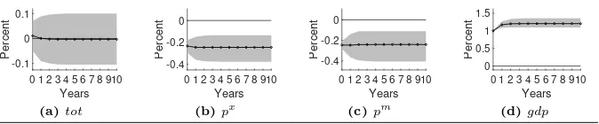
Figure 1 displays the impulse response functions (IRFs) of the terms of trade (denoted bytot), the export unit value index (denoted bypx), the import unit value index (denoted bypm), and output per employed person (denoted by_gdp) to a positive productivity shock, resulting in an unexpected one percent increase in output per employed person in the impact period.7 _{In Figure 1, the IRFs of}

pmare calculated by subtracting the IRFs of the terms of trade (_tot) from those of the export unit value index (px). As is evident from Figure 1, we find that a positive productivity shock

• results in an insignificant change in the terms of trade in both advanced and developing economies;

7_{An impulse response of a variable shows the change in the variable caused by the}

Panel A: Advanced Economies

0 1 2 3 4 5 6 7 8 910 Years -0.1 0 0.1 Percent (a)tot

0 1 2 3 4 5 6 7 8 910

Years

-0.4 -0.2 0

Percent

(b)px

0 1 2 3 4 5 6 7 8 910 Years -0.4 -0.2 0

Percent

(c)pm

0 1 2 3 4 5 6 7 8 910

Years 0 0.5 1 1.5 Percent (d)gdp

Panel B: Developing Economies

0 1 2 3 4 5 6 7 8 910

Years -0.1 0 0.1 Percent (a)tot

0 1 2 3 4 5 6 7 8 910

Years -0.2 -0.1 0 0.1 Percent

(b)px

0 1 2 3 4 5 6 7 8 910 Years -0.2 -0.1 0 0.1 Percent

(c)pm

0 1 2 3 4 5 6 7 8 910 Years 0 0.5 1 1.5 Percent (d)gdp

Note:Our calculations are based on the World Bank’sWorld Development Indicators. Solid lines with diamonds indicate the median IRFs. Grey areas are 68 percent confidence intervals estimated using the Monte Carlo method presented in appendix C.

Figure 1: IRFs to a Positive Productivity Shock

(Baseline Results)

• gives rise to a large and persistent fall and a largely insignificant and transitory fall in the export unit value index in advanced and developing economies, respectively;

• causes a large fall and an insignificant change in the import unit value index in advanced and developing economies, respectively; and

• induces a permanent increase in output per employed person in advanced and developing economies, which is significant at all horizons that we compute the IRFs.

Panel A: Advanced Economies

0 1 2 3 4 5 6 7 8 910 Years -0.2 -0.1 0 0.1 Percent (a)tot

0 1 2 3 4 5 6 7 8 910 Years -0.4

-0.2 0

Percent

(b)px

0 1 2 3 4 5 6 7 8 910 Years -0.4

-0.2 0

Percent

(c)pm

0 1 2 3 4 5 6 7 8 910

Years 0 0.5 1 1.5 Percent (d)gdp

Panel B: Developing Economies

0 1 2 3 4 5 6 7 8 910

Years -0.2 0 0.2 Percent (a)tot

0 1 2 3 4 5 6 7 8 910 Years -0.3 -0.2 -0.1 0 0.1 Percent

(b)px

0 1 2 3 4 5 6 7 8 910

Years

-0.2 0 0.2

Percent

(c)pm

0 1 2 3 4 5 6 7 8 9 10 Years 0 1 2 Percent (d)gdp

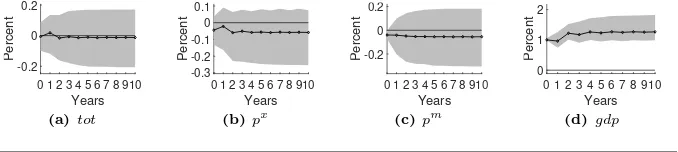
Note:Our calculations are based on the World Bank’sWorld Development Indicators. Solid lines with diamonds indicate the median IRFs. Grey areas are 68 percent confidence intervals estimated using the Monte Carlo method presented in appendix C.

Figure 2: IRFs to a Positive Productivity Shock

(First Robustness Check: An Alternative Specification with¯_{k= 2, H= 10)}

4.2 Robustness Checks

4.2.1 Different Model Specifications

In this section, we consider two robustness checks. In the first robustness check, we use the specification thatH= 10and¯k= 2. Consequently, in this alternative

specification, while the horizon at which the forecast-error variance share of productivity in output per employed person is maximized is the same as in the benchmark specification, we allow for richer dynamics by selecting the lag length in Model (2.3) as two instead of one as in the benchmark specification.

Figure 2 displays the IRFs from the alternative specification allowing for richer dynamics. It is discernible that the fall in the terms of trade in ad-vanced economies is more pronounced under this specification than under the benchmark specification; see Figure 1 and Figure 2. Apart from this, the re-sults differ little between the two specifications. Consequently, the rere-sults under this alternative specification are also consistent with the small-country assump-tion for developing economies when considered as a whole. They reject the Prebisch-Singer hypothesis, however, more strongly. Indeed, they indicate that a positive productivity shock causes more unfavorable terms-of-trade dynamics in advanced economies than in developing economies, let alone causing less unfa-vorable terms-of-trade dynamics in the former, as implied by the Prebish-Singer hypothesis.

As a second robustness check, the specification that H = 20 and ¯k = 1is

considered. In this alternative specification, while the lag length in Model (2.3) is the same as in the benchmark specification, the anticipation horizon is longer than that in the benchmark specification. Since the results implied by this alternative specification are almost identical to those implied by the benchmark specification, they are not reported for reasons of brevity.8

Panel A: Advanced Economies

Benchmark Specification(¯k= 1, H= 10) Alternative Specification(¯k= 2, H= 10)

0 1 2 3 4 5 6 7 8 910 Years -0.1 0 0.1 Percent (a)tot

0 1 2 3 4 5 6 7 8 910 Years -0.3 -0.2 -0.1 0 0.1 Percent

(b)px

0 1 2 3 4 5 6 7 8 910

Years -0.3 -0.2 -0.1 0 0.1 Percent

(c)pm

0 1 2 3 4 5 6 7 8 910

Years -0.2 -0.1 0 0.1 Percent (d)tot

0 1 2 3 4 5 6 7 8 910 Years -0.4 -0.2 0

Percent

(e)px

0 1 2 3 4 5 6 7 8 910

Years -0.3 -0.2 -0.1 0 0.1 Percent

(f)pm

Panel B: Developing Economies

Benchmark Specification(¯k= 1, H= 10) Alternative Specification(¯k= 2, H= 10)

0 1 2 3 4 5 6 7 8 910

Years -0.1 0 0.1 Percent (a)tot

0 1 2 3 4 5 6 7 8 910

Years -0.1 0 0.1 0.2 Percent

(b)px

0 1 2 3 4 5 6 7 8 910

Years -0.1 0 0.1 0.2 Percent

(c)pm

0 1 2 3 4 5 6 7 8 910

Years 0 0.2 0.4 Percent (d)tot

0 1 2 3 4 5 6 7 8 910 Years -0.1 0 0.1 0.2 0.3 Percent

(e)px

0 1 2 3 4 5 6 7 8 910 Years -0.2

0 0.2

Percent

(f)pm

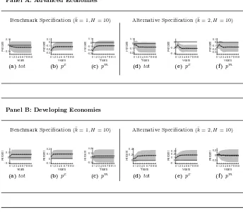
Note:Our calculations are based on the World Bank’sWorld Development Indicators. Solid lines with diamonds indicate the median IRFs. Grey areas are 90 percent confidence intervals estimated using the Monte Carlo method presented in appendix C.

Figure 3: IRFs to a Positive Productivity Shock

(Second Robustness Check: Extended Sample Period)

4.2.2 Results from a Longer Sample Period

In this section, we extend our sample period back to 1991 for developing and advanced economies and discuss the results under both the benchmark spec-ification and the specspec-ification that allows for richer dynamics. It is notable that the responses to a productivity shock can be more preciously estimated

when the sample period is extended back to 1991. However, doing so results in an unbalanced panel since data is available only for a small fraction of ad-vanced economies and about half of developing economies between 1991-1999. To eliminate the sample selection bias, the additional assumption that selection is unrelated to the idiosyncratic errorsui,t in Model (2.3) must be made for the longer unbalanced panel; see Wooldridge (2002, chapter 17.7). Our decision to study the sample period of 2000-2016 in our main analysis stems from the fact that our panel for 2000-2016 is balanced, and, by construction, free of sample-selection bias, which may plague the results from the longer unbalanced panel if the assumption that selection is unrelated to the idiosyncratic errors is violated. It is also notable that in the unbalanced panel, estimating common factors in Model(2.3) requires imputing some missing values. We impute these values using the expectation-maximization algorithm suggested by Stock and Watson (2002) and Bai (2009). As simulation studies done in Bai, Liao, and Yang (2015) show, this algorithm yields consistent estimates, converging rapidly to their true values for both smooth and stochastic factors.

Before discussing the results from the longer sample, a caveat must be dis-cussed. Four out of 36 advanced economies in our sample have data between 1991-1999, resulting in the unbalanced panel of advanced economies having only 36 more observations than the balanced panel of advanced economies. Conse-quently, a small gain in precision from extending the sample period back to 1991 may not be worth the risk of introducing sample-selection bias in the estimates from the unbalanced panel, causing them to be inconsistent.

Panel Aof Figure 3 illustrates the IRFs to a positive productivity shock in advanced economies from the unbalanced panel as estimated using the bench-mark specification and the specification that allows for richer dynamics (¯_{k= 2).}

¯

kand are similar to those seen in the shorter balanced panel. First, the terms of

trade in advanced economies show insignificant dynamics after a positive pro-ductivity shock. Second, the export and import prices in advanced economies experience a large fall after the shock.

Panel Bof Figure 3 displays the IRFs to an unexpected increase in produc-tivity in developing economies in the unbalanced panel as estimated using the aforementioned specifications. In the unbalanced panel, the IRFs of the terms of trade in developing economies in the benchmark specification are not signif-icant. This finding is consistent with our baseline results. In the specification allowing for richer dynamics, on the other hand, the terms of trade in developing economies show barely significant increases after a positive productivity shock, caused largely by an increase in the export prices. This finding slightly differs from the baseline results and provide some weak evidence against both the small-country assumption and the Prebisch-Singer hypothesis since while the former predicts no terms-of-trade change, the latter predicts a definite terms-of-trade decline following such a shock in developing economies.

4.2.3 TFP at Constant National Prices as a Different Measure of Productivity

In our main analysis, we opted to use output per employed person as a mea-sure of productivity due to the larger availability of data for a large number of economies. However, a better measure of productivity in an economy is to-tal factor productivity at constant national prices (denoted bytf pit), on which

Feenstra, Inklaar, and Timmer (2015) have data only for about half of the economies included in our sample; see Table A.1.

In-Panel A: Advanced Economies

Shorter Balanced Panel (2000-2014) Longer Unbalanced Panel (1980-2014)

0 1 2 3 4 5 6 7 8 910

Years -0.2 -0.1 0 0.1 Percent

(a)k¯=1,H=10

0 1 2 3 4 5 6 7 8 910

Years

-0.2 0 0.2

Percent

(b)k¯=2,H=10

0 1 2 3 4 5 6 7 8 910

Years -0.3 -0.2 -0.1 0 0.1 Percent

(c)¯k=1,H=10

0 1 2 3 4 5 6 7 8 910

Years -0.2 -0.1 0 0.1 Percent

(d)¯k=2,H=10

Panel B: Developing Economies

Shorter Balanced Panel (2000-2014) Longer Unbalanced Panel (1980-2014)

0 1 2 3 4 5 6 7 8 910

Years -0.4 -0.2 0 0.2 Percent (a) tot

(¯k=1,H=10)

0 1 2 3 4 5 6 7 8 910

Years -0.6 -0.4 -0.2 0 0.2 Percent (b) tot

(¯k=2,H=10)

0 1 2 3 4 5 6 7 8 910

Years -0.1 0 0.1 0.2 0.3 Percent (c) tot

(¯k=1,H=10)

0 1 2 3 4 5 6 7 8 910 Years -0.2 0 0.2 Percent (d) tot

(¯k=2,H=10)

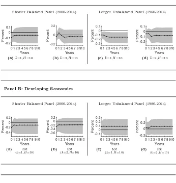
Note: Our calculations are based on data from the World Bank’sWorld Development In-dicatorsand Feenstra, Inklaar, and Timmer (2015). Solid lines with diamonds indicate the median IRFs. Grey areas are 90 percent confidence intervals estimated using the Monte Carlo method presented in appendix C.

Figure 4: IRFs of the Terms of Trade to a Positive Productivity Shock

(Third Robustness Check: TFP as a Different Productivity Measure)

deed, we obtain the results from both the benchmark specification, given by

¯

k= 1, H = 10, and the alternative specification allowing for richer dynamics,

spanning the period of 2000-2014 and the unbalanced panel spanning the period of 1980-2014 with about half of the developing economies and only four of the advanced economies in our sample having data between 1980-1999. Figure 4 shows the IRFs of the terms of trade to a productivity shock identified by se-lectingtf pitas a measure of productivity.9 Apart from a decisive terms-of-trade fall in advanced economies when the benchmark specification in the unbalanced panel is considered, the IRFs of the terms of trade in Figure 4 are largely similar to the baseline results displayed in Figure 1.

4.3 A More Detailed Classification of Developing

Economies

neous dynamics in the group of developing economies. We study this question by further dividing this group into two sub-groups: the developing economies with a high degree of export diversification—whose average index between the years 2000 and 2010 ranks in the first quartile of the IMF’sexport diversification index

among developing economies—and the remaining developing economies which have a lower degree of export diversification. The numbers of the economies in the former and the latter are 33 and 98, respectively.10 _{Table A.1 in the}

appendix presents the economies on the list of the developing economies with a high degree of export diversification.

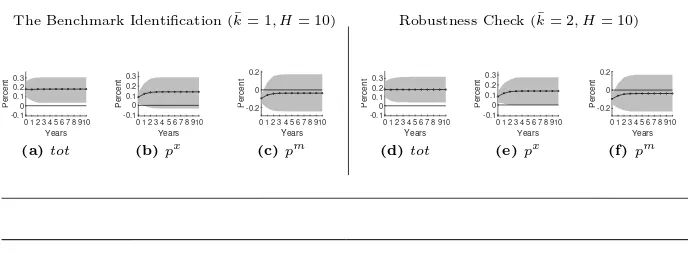
Figure 5 displays the IRFs of the variables to a positive productivity shock in the developing economies with a high degree of export diversification and the remaining developing economies.11 _{Consistent with the previous analysis,}

we consider the benchmark specification given by (¯k = 1, H = 10) and the

specification with richer dynamics given by (¯k = 2, H = 10). Regarding the

developing economies with a high degree of export diversification, we find that an unexpected increase in productivity leads to an improvement in the terms of trade.12 _{In contrast, an unexpected increase in productivity in the remaining}

developing economies results in no significant change in the terms of trade. As a second robustness check, we consider the longer sample period of 1991-2016. Since data is unavailable for a large number of developing economies between 1991-1999, the panel is unbalanced. Consequently, the consistency 10_{Data on the export diversification index is available for 131 out of 141 developing economies}

in our sample. In this section, we only include the developing economies having data on the export diversification index.

11_{The analysis similar to appendix B indicates that gdp, tot, and p}x _{in the developing} economies with a high degree of export diversification and the remaining developing economies are of order one and there is no stationary linear combination of the series. Consequently, the panel VAR model is specified in first-differences to eliminate all non-standard distributions that would result were the model specified in levels. The results are not reported for reasons of brevity.

12_{For the sake of brevity, the IRFs of output per employed person, which stay positive and}

Panel A: Developing Economies with a High Degree of Export Diversification

The Benchmark Identification(¯k= 1, H= 10) Robustness Check(¯k= 2, H= 10)

0 1 2 3 4 5 6 7 8 910 Years 0 0.2 0.4 Percent (a)tot

0 1 2 3 4 5 6 7 8 910

Years -0.1 0 0.1 0.2 0.3 Percent

(b)px

0 1 2 3 4 5 6 7 8 910

Years -0.3 -0.2 -0.1 0 0.1 Percent

(c)pm

0 1 2 3 4 5 6 7 8 910

Years 0 0.2 0.4 0.6 Percent (d)tot

0 1 2 3 4 5 6 7 8 910 Years 0 0.2 0.4

Percent

(e)px

0 1 2 3 4 5 6 7 8 910

Years

-0.4 -0.2 0

Percent

(f)pm

Panel B: Remaining Developing Economies

The Benchmark Identification(¯k= 1, H= 10) Robustness Check(¯k= 2, H= 10)

0 1 2 3 4 5 6 7 8 910

Years -0.2 -0.1 0 0.1 Percent (a)tot

0 1 2 3 4 5 6 7 8 910

Years -0.2 -0.1 0 0.1 Percent

(b)px

0 1 2 3 4 5 6 7 8 910

Years -0.2 -0.1 0 0.1 Percent

(c)pm

0 1 2 3 4 5 6 7 8 910 Years -0.3 -0.2 -0.1 0 0.1 Percent (d)tot

0 1 2 3 4 5 6 7 8 910

Years -0.3 -0.2 -0.1 0 0.1 Percent

(e)px

0 1 2 3 4 5 6 7 8 910

Years

-0.2 0 0.2

Percent

(f)pm

Note:Our calculations are based on the World Bank’sWorld Development Indicators. Solid lines with diamonds indicate the median IRFs. Grey areas are 90 percent confidence intervals estimated using the Monte Carlo method presented in appendix C.

Figure 5: IRFs to a Positive Productivity Shock

(Baseline Results and First Robustness Check)

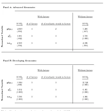
of the results requires the additional assumption that selection is unrelated to idiosyncratic errors. The IRFs to an unexpected increase in productivity in the developing economies with a high degree of export diversification and the remaining developing economies as estimated using both of the aforementioned specifications in the unbalanced panel are shown, respectively, byPanel Aand

Panel A: Developing Economies with a High Degree of Export Diversification

The Benchmark Identification(¯k= 1, H= 10) Robustness Check(¯k= 2, H= 10)

0 1 2 3 4 5 6 7 8 910

Years -0.1 0 0.1 0.2 0.3 Percent (a)tot

0 1 2 3 4 5 6 7 8 910 Years -0.1 0 0.1 0.2 0.3 Percent

(b)px

0 1 2 3 4 5 6 7 8 910

Years

-0.2 0 0.2

Percent

(c)pm

0 1 2 3 4 5 6 7 8 910 Years -0.1 0 0.1 0.2 0.3 Percent (d)tot

0 1 2 3 4 5 6 7 8 910 Years -0.1 0 0.1 0.2 0.3 Percent

(e)px

0 1 2 3 4 5 6 7 8 910 Years -0.2

0 0.2

Percent

(f)pm

Panel B: Remaining Developing Economies

The Benchmark Identification(¯k= 1, H= 10) Robustness Check(¯k= 2, H= 10)

0 1 2 3 4 5 6 7 8 910 Years -0.1 0 0.1 Percent (a)tot

0 1 2 3 4 5 6 7 8 910 Years -0.1 0 0.1 0.2 Percent

(b)px

0 1 2 3 4 5 6 7 8 910 Years -0.1 0 0.1 0.2 Percent

(c)pm

0 1 2 3 4 5 6 7 8 910 Years -0.1 0 0.1 Percent (d)tot

0 1 2 3 4 5 6 7 8 910 Years -0.1 0 0.1 0.2 Percent

(e)px

0 1 2 3 4 5 6 7 8 910 Years -0.1 0 0.1 0.2 Percent

(f)pm

Note:Our calculations are based on the World Bank’sWorld Development Indicators. Solid lines with diamonds indicate the median IRFs. Grey areas are 90 percent confidence intervals estimated using the Monte Carlo method presented in appendix C.

Figure 6: IRFs to a Positive Productivity Shock

(Second Robustness Check: Extended Sample Period)

this section that the terms of trade experience a significant improvement in the developing economies with a high degree of export diversification following an unexpected increase in productivity is robust to extending the sample period and using an alternative specification with richer dynamics.

Panel A: Developing Economies with a High Degree of Export Diversification

Shorter Balanced Panel (2000-2014) Longer Unbalanced Panel (1980-2014)

0 1 2 3 4 5 6 7 8 910

Years 0 0.2 0.4 Percent (a) tot

(¯k=1,H=10)

0 1 2 3 4 5 6 7 8 910

Years -0.2 0 0.2 0.4 Percent (b) tot

(¯k=2,H=10)

0 1 2 3 4 5 6 7 8 910

Years 0 0.2 0.4 0.6 0.8 Percent (c) tot

(¯k=1,H=10)

0 1 2 3 4 5 6 7 8 910

Years 0 0.2 0.4 0.6 0.8 Percent (d) tot

(¯k=2,H=10)

Panel B: Remaining Developing Economies

Shorter Balanced Panel (2000-2014) Longer Unbalanced Panel (1980-2014)

0 1 2 3 4 5 6 7 8 910

Years -0.6 -0.4 -0.2 0 0.2 Percent (a) tot

(¯k=1,H=10)

0 1 2 3 4 5 6 7 8 910 Years -1 -0.5 0 Percent (b) tot

(¯k=2,H=10)

0 1 2 3 4 5 6 7 8 910 Years -0.3 -0.2 -0.1 0 0.1 Percent (c) tot

(¯k=1,H=10)

0 1 2 3 4 5 6 7 8 910 Years -0.2 0 0.2 Percent (d) tot

(¯k=2,H=10)

Note: Our calculations are based on data from the World Bank’sWorld Development In-dicatorsand Feenstra, Inklaar, and Timmer (2015). Solid lines with diamonds indicate the median IRFs. Grey areas are 90 percent confidence intervals estimated using the Monte Carlo method presented in appendix C.

Figure 7: IRFs of the Terms of Trade to a Positive Productivity Shock

(Third Robustness Check: TFP as a Different Productivity Measure)

mon finding in this analysis is that an increase in productivity is associated with a significant terms-of-trade improvement (no significant terms-of-trade change) in the developing economies with a high degree of export diversification (the re-maining developing economies).14 _{This finding provides evidence against both}

the small-country assumption and the Prebisch-Singer hypothesis. Its critical significance in the literature lies in that putting all developing economies in the same basket can be misleading since the developing economies with a high degree of export diversification can positively distinguish themselves from the remaining developing economies regarding the effect of productivity shocks on the terms of trade.

5 Discussion and Conclusions

In this paper, we studied the effects from economy-specific shocks to productiv-ity on the terms of trade with a focus on developing economies. We obtained the results with the various model specifications, the different sample periods, and the different measures of productivity. Our robust finding in this analysis is that such an increase results in insignificant dynamics in the terms of trade in both developing and advanced economies. While this finding support the small-country assumption for developing economies when considered as a whole, it rejects the Prebisch-Singer hypothesis, predicting more adverse terms-of-trade dynamics in developing economies than in advanced economies following a sur-prise increase in productivity. However, studying the terms-of-trade effects from a positive economy-specific shock to productivity in a more detailed classifica-tion of developing economies revealed another robust finding in our study that 14_{The only exception is the results from the specification(¯k= 2, H= 10)in the unbalanced}

such a shock is associated with a significant improvement in the terms of trade in the developing economies with a high degree of export diversification.

Consequently, it is questionable to maintain the small-country assumption for the developing economies with a high degree of export diversification. An essential step to accounting for our finding of a significant appreciation in the terms of trade after a positive economy-specific shock to productivity in these economies is to drop the assumption that they export homogeneous products, as implied by the small-country assumption in the literature and assume instead that they also produce differentiated products in international markets. This can be based on the fact that the share of differentiated goods exported by the developing world to the OECD countries increased considerably between 1980 and 2006, as noted in Artopoulos, Friel, and Hallak (2013). This can result either from the success of some developing economies to move up in the ladder of economic development or simply from these economies involving in the low-skill assembly stages of global production chains organized by multinational firms headquartered in the developed world.

models with suitable calibration of model parameters. For example, Corsetti, Dedola, and Leduc (2008) show in such a model that a sufficiently low trade price elasticity together with substantial home bias in consumption can result in an increase in productivity causing a permanent appreciation in the terms of trade. This results from the demand for domestic goods raising above supply due to strong wealth effects brought about by increased productivity.

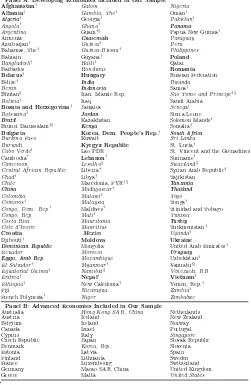
Appendix A Economies in Our Sample

Panel A. Developing Economies included in Our Sample

Afghanistan† _{Gabon Nigeria}

Albania† _{Gambia, The}† _Oman†

Algeria† _Georgia† _Pakistan†

Angola† _Ghana† _Panama

Argentina Guam†§ _{Papua New Guinea}†

Armenia Guatemala Paraguay

Azerbaijan† _Guinea† _Peru

Bahamas, The† _{Guinea-Bissau}† _Philippines

Bahrain Guyana† _Poland

Bangladesh† _Haiti† _Qatar

Barbados Honduras Romania

Belarus† _{Hungary Russian Federation}

Belize† _{India Rwanda}

Benin Indonesia Samoa†

Bhutan§ _{Iran, Islamic Rep. Sao Tome and Principe}†§

Bolivia† _{Iraq Saudi Arabia}

Bosnia and Herzegovina† _{Jamaica Senegal}

Botswana§ _{Jordan Sierra Leone}

Brazil Kazakhstan Solomon Islands†

Brunei Darussalam†§ _{Kenya Somalia}†

Bulgaria Korea, Dem. People’s Rep.† South Africa

Burkina Faso Kuwait Sri Lanka

Burundi Kyrgyz Republic St. Lucia†

Cabo Verde† _{Lao PDR St. Vincent and the Grenadines}†

Cambodia† _Lebanon† _Suriname†

Cameroon Lesotho§ _Swaziland§

Central African Republic Liberia† _{Syrian Arab Republic}†

Chad† _Libya† _Tajikistan

Chile Macedonia, FYR†§ _Tanzania

China Madagascar† Thailand

Colombia Malawi† _Togo

Comoros† _{Malaysia Tonga}†

Congo, Dem. Rep.† _Maldives† _{Trinidad and Tobago}

Congo, Rep. Mali† _Tunisia

Costa Rica Mauritania Turkey

Cote d’Ivoire Mauritius Turkmenistan†

Croatia Mexico Uganda†

Djibouti† _{Moldova Ukraine}

Dominican Republic Mongolia United Arab Emirates†

Ecuador Morocco Uruguay

Egypt, Arab Rep. Mozambique Uzbekistan†

El Salvador† _Myanmar† _Vanuatu†§

Equatorial Guinea† _Namibia§ _{Venezuela, RB}

Eritrea† _Nepal† _Vietnam†

Ethiopia† _{New Caledonia}† _{Yemen, Rep.}†

Fiji Nicaragua Zambia†

French Polynesia† _{Niger Zimbabwe}

Panel B: Advanced Economies Included in Our Sample

Australia Hong Kong SAR, China Netherlands

Austria Iceland New Zealand

Belgium Ireland Norway

Canada Israel Portugal

Cyprus Italy Singapore

Czech Republic Japan Slovak Republic

Denmark Korea, Rep. Slovenia

Estonia Latvia Spain

Finland Lithuania Sweden

France Luxembourg Switzerland

Germany Macao SAR, China United Kingdom

Greece Malta United States

Note:

• The sample period of those economiesemphasizedis 1991-2016. Economies not emphasized have data between 2000-2016.

• Economies inboldcharacters are the developing economies ranking in the first quartile of the IMF’sExport Diversification Index among developing economies between 2000-2010.

• Economies with a † are the developing economies whose data on TFP at constant national prices is unavailable.

• Economies with a§are the developing economies whose data on the IMF’s Export Diversification Index is unavailable.

Appendix B Specifications Issues

While estimating a vector autoregression often provides a convenient way of describ-ing dynamics of variables, it involves makdescrib-ing a number of critical decisions which may have a significant impact on inference. For example, when some variables included in the VAR contain a unit root, should they be included in levels or in differences? Hamilton (1994, p. 651-653) discusses this issue in detail. He notes if the true pro-cess is VAR in differences, differencing should improve the small-sample performance of all estimates and can eliminate non-standard distributions associated with certain hypothesis testing. However, differencing all variables in a VAR can result in a mis-specified regression in such cases where some variables are already stationary or there is a stationary linear relationship betweenI(1)variables included in the VAR.15

We represent our system with a panel VAR with interactive fixed effects in differ-ences based on two findings. First, using a panel unit root test, we reveal all variables included in our panel VAR model areI(1). Second, we show that there is no linear combination of the variables which is stationary.

B.1 Panel Unit Root Tests in the Presence of Common

Shocks

We investigate whether the series’ contain a unit root or not using the modified Sar-gan–Bhargava test (theM SBtest) proposed by Stock (1999) and discussed extensively

in Bai and Carrion-I-Silvestre (2009) and Bai and Ng (2010) in the context of a panel data with cross-sectional dependence. The model on which theMSBtest is based is given by

yi,t = µi+νit+f

′

tλi+ui,t

i= 1,2, . . . , N ; t= 1,2, . . . , T

(B.1)

whereyi,tdenotes one of the three variables contained inYi,t. µi andνirepresent

economy-specific intercept and trend terms, respectively. λi, ft, and ui,t represent

15_{In fact, as shown in Hamilton (1994, p. 574-575), a cointegrated system cannot be}

factor loadings, common factors, and idiosyncratic errors, respectively.

The error structure in theMSBtest is useful for two reasons. First, it is notable that since λi is an economy-specific parameter, the error structure allows common

shocks to have a different effect on individual economies. This assumption is useful in our analysis since common shocks can affect individual economies differently. For example, the unprecedented increase in the IMF’s crude oil price index from its trough of 19.54 to its peak of 249.66 between 1998:12 and 2008:7 can be regarded as a global oil shock. It may be argued that while this shock favorably affected the terms of trade of oil-exporting economies, it had an unfavorable effect on the terms of trade of oil-importing economies. Second, since common shocks are likely to cause high cross-section dependence, the assumption of uncorrelated error terms across countries, as in Choi (2001), would result in large size distortion; see Pesaran (2007).

One can write the differenced form of (B.1) in matrix notation as

∆yi = ιTνi+ ∆f λi+ ∆ui

i= 1,2, . . . , N ; t= 2,3, . . . , T

(B.2)

where ιT is a T×1vector of ones. Let MιT =IT−

1 TιTι

′

T. Multiplying (B.2) withMι_T eliminates the constant from this equation:

∆y∗

i,t = ∆f

∗′

t λi+ ∆u

∗

i,t

i= 1,2, . . . , N ; t= 2,3, . . . , T

(B.3)

where∆y∗

i,t=Mι_T∆yi,t,∆f

∗

t =Mι_T∆ft, and∆u

∗

i,t=Mι_T∆ui,t. Letuˆ

∗

i,tbe the

least squares estimates ofPT s=2∆u

∗

i,s. TheM SBu¯∗(i)test statistics is defined by

M SBu¯∗(i) =

(T−2)2

T

P

t=3 ˆ u∗2

i,t−₁

ˆ

σ2

u∗

i

(B.4)

where ˆσ2u∗

i denotes an estimator of the long-run variance ofu

∗

i. As suggested by

Bai and Carrion-i Silvestre (2013),σˆu2∗

i can be estimated as

ˆ σ2u∗

i =

ˆ

σ2

ki,i

1−φbi,1

withˆσ2ki,i= (T−3)

−₁PT

t=4νˆi,t, whereφbi,1andνˆi,tare the least squares estimates

from the following equation:

∆ˆu∗

i,t = φi,0uˆ∗i,t−₁+φi,1∆ˆu∗i,t−₁+νi,t

i= 1,2, . . . , N ; t= 4,5, . . . , T

(B.6)

The MSB test discussed in Bai and Carrion-I-Silvestre (2009), which asymptoti-cally has standard normal distribution, is given by

M SBu¯∗ = √N

M SBu¯∗₋1

6

p₁

45

(B.7)

withM SBu¯∗=N−1PN

i=1M SBu¯∗(i).

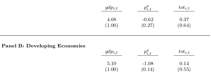
Panel A andPanel B of Table B.1 report the MSB test statistics ofgdpi,t,pxi,t,

andtoti,tfor advanced and developing economies, respectively. It is notable that when

obtaining theM SBu¯∗ test statistics, the number of common factors in (B.3) is treated

as unknown and is estimated using the eigenvalue ratio estimator suggested by Ahn and Horenstein (2013) allowing up to five common factors. The number of factors selected based on the eigenvalue ratio estimator is one forgdpi,t,pxi,t, andtoti,tin our

sample of both advanced and developing economies. From thep-values reported in

Panel A, it is evident that the null hypothesis of a unit root in neithergdpi,t, norpxi,t,

and nortoti,tacross all advanced economies cannot be rejected. Similarly, we fail to

reject the null in the sample of developing economies forgdpi,t,pxi,t, andtoti,t since

the p-values of theM SBu¯∗ test statistics reported in Panel B are larger than the 5%

significance level selected in our analysis.

B.2 A Panel Cointegration Test in the Presence of

Com-mon Shocks

Can there be a linear combination of gdpi,t, pxi,t, and toti,t that is stationary and

suggests a long-run equilibrium relationship between gdpi,t, pxi,t, and toti,t despite

Panel A: Advanced Economies

gdpi,t pxi,t toti,t

4.68 -0.62 0.37

(1.00) (0.27) (0.64)

Panel B: Developing Economies

gdpi,t pxi,t toti,t

5.10 -1.08 0.14

(1.00) (0.14) (0.55)

Note: Panel A and Panel B report theMSBtest statistics of thelog-level of the variables for advanced and developing economies, respectively. Numbers in parenthesis refer to the p-values of theMSBtest statistics.

Table B.1: Panel Unit Root Test Results

cointegrated? The answer to this question is instrumental in specifying the panel VAR model discussed in section 2.1. Indeed, when a linear combination of the series is stationary, the level specification must be preferred since a panel VAR in differences is not consistent with a cointegrated system, as shown in Hamilton (1994). Before explaining how we test for cointegration, it is useful to review two well-known economic models related to the terms of trade determination: a standard international macro model with differentiated goods and the Prebisch-Singer model. In the former, the terms of trade between any two countries are largely determined by differences in productivity in their tradable sectors and an increase in productivity is most likely associated with a fall in export prices. The latter argues that apart from differences in productivity in tradables sectors, the goods and labor market structures also play a key role in the determination of the terms of trade. Indeed, according to the latter, the effect that increased productivity has on export prices would be more unfavorable in economies with more competitive goods and labor markets. Cangdpi,t,pxi,t, andtoti,t

common factors, the answer is more complex. Indeed, when common factors are added to the analysis, a measure of changes in productivity in the foreign trade sector can be reflected in a linear combination of common factors, possibly yielding that a long-run relationship betweengdpi,t,pxi,t, andtoti,tcan exist up to some common global trends

represented by these factors.

Next, we discuss the issue from the statistical point of view. We test whether the series in our analysis are cointegrated with the panel cointegration test developed by Bai and Carrion-i Silvestre (2013), which allows cross-sectiona