Munich Personal RePEc Archive
Optimal Value-at-Risk Disclosure
Seixas, Mário and Barbosa, António
Banco de Portugal, ISCTE - Instituto Universitário de Lisboa
2019
Optimal Value-at-Risk Disclosure
Mário Seixas
Banco de Portugal
António Barbosa∗
ISCTE-IUL - Instituto Universitário de Lisboa
This version: December 2019
Abstract
In 1995, the Basel Accords introduced an alternative method to compute the mar-ket risk charge through the use of a risk model developed internally by the financial institution. These internal models, based on the Value-at-Risk (VaR), follow certain rules that are defined under the Basel Accords. From this moment on, risk analysts and financial academics focused their attentions on how to accurately estimate the VaR in order to reduce the regulatory capital. However, considering the market risk framework defined in the Basel Accords, the best strategy to optimize the regulatory capital may not lie in truthfully disclosing an accurate VaR estimation. In this study, we propose to solve, through dynamic programming, for the optimal policy function for disclosing the reported VaR based on the estimated value that minimizes the daily capital charge. This policy function will provide the optimal percentage of the esti-mated 1-day VaR that should be disclosed, taking into account the impact that this disclosure decision will have in future capital charges, by managing the rules defined in the Basel Accords. Our goal is to prove that truthful disclosure of an accurately estimated VaR is suboptimal. The main results from our investigation show that us-ing the optimal reportus-ing strategy leads to an average daily reduction in the capital requirements of 4.32% in a simulated environment, compared with a normal strategy of always truthfully disclosing the estimated 1-day VaR, and leads to an average daily saving of 7.22% when applied to our S&P500 test portfolio.
JEL Classification: G32, G28, G11, G17
Keywords: Value-at-Risk, Regulatory Capital, Market Risk Charge, Optimal Disclosure, Dynamic Programming
∗
1
Introduction
In 1995, the Basel Committee on Banking Supervision (BCBS) introduced an internal model to compute the market risk – Value-at-Risk (VaR) – and define the regulatory capital charge used to cover future losses related to this type of risk. This model was described as the estimate for the worst possible loss that a certain portfolio could suffer considering a predetermined statistical confidence (Basel Committee on Banking Supervison, 1995).
Since then, the Basel Accords, and the VaR method, were adopted by more than 100 countries (Alexander, 2008). Due to this worldwide use, there exists a big literature on this topic and, in particular, about the methods to estimate the VaR (Angelovska, 2013; Aussenegg and Miazhynskaia, 2006; Hull and White, 1998; Totić et al., 2011; and Ünal, 2011).
However, as far as we know, there exists few literature on possible strategies to optimize the daily capital charge based on VaR internal models. Some of these studies focus on the idea that the best method to optimize the daily capital charge is by accurately estimating the VaR (McAleer, 2009), while others explored the use of financial options to minimize VaR and, consequently, the capital charge (Ahn et al., 1999; and Deelstra et al., 2007).
Nevertheless, there is one study that stands out from the others that was introduced by McAleer et al. (2010). In it, the authors developed a function that minimizes the daily capital charge through the management of the number of exceedances (i.e. number of days where the actual loss exceeds the VaR estimate) that a financial institution (FI) is allowed to have, according to the Basel rules (Basel Committee on Banking Supervison, 1995). With this model, risk analysts obtain the optimal percentage of the forecasted VaR that should be reported taking into account two variables: the number of exceedances recorded since the beginning of the regulatory period; and the number of exceedances recorded in the last 25 days.
The authors reached the conclusion that using their function together with a VaR model could reduce the daily capital charges up to 14.3% when compared with the RiskMetrics Model.1
However, to achieve the perfect model it is necessary to do a calibration test for the parameters, which is computational intensive and time consuming, and no out-of-sample tests were performed in order to verify if this would work in a real life context.
Considering this and the small number of studies in this field, we propose to create a model for the optimization of the regulatory capital charge by choosing the VaR disclosure based on the estimated VaR and other key variables. This optimal disclosure policy is solved using dynamic programming methods.
Dynamic programming is a method to solve for optimization problems that can be stated recursively. The solution that is obtained is a policy function that defines the optimal course of action in each possible state of nature, taking into consideration the effect of those choices in the future.
1
In the case of our model, the policy function represents the percentage of the estimated 1-day VaR that should be disclosed, and this optimal decision will depend on three state variables which, together, fully describe the state of nature: time remaining for the regu-lator to do the backtesting and review the multiplier (TtoB); multiplier that is currently in use (K); and the number of exceedances that were recorded until the moment of the decision, during the current regulatory period (EC). For each combination of these state variables, there exists an optimal decision that optimizes today’s capital charge taking into account the effect that this decision will have in the likelihood of future states of nature and, as a consequence, in future capital charges. The range of these variables was chosen according to the rules defined by the Basel Accords for the use of internal models (Basel Committee on Banking Supervison, 1995).
This problem will be solved as an infinite horizon Markov decision process with the use of the function iteration algorithm on MATLABTM
software.
The advantage of our model is the elimination of any subjective choice or calibration need for the parameters, defining the optimal policy according to the maximization of a value function that represents the present value of a FI’s capital charges (that has a negative sign), which are directly related to the FI’s cost of capital.
In a general way, the results of the optimal policy point out to an aggressive strategy when exceedances are low, i.e. underreport the estimated VaR, and to a more conservative strategy when exceedances are high, i.e. overreport the estimated VaR. There are some deviations from this general strategy that will be analyzed later on in Section 4.
The results from this model will then be tested in a Monte Carlo simulation and afterwards they will be applied to a real portfolio in order to compare the performance of the optimal reporting strategy (i.e. reporting the 1-day VaR according to the optimal policy) with that of a strategy that truthfully reports the estimated VaR. The main results from these 2 analyses were very promising. In the Monte Carlo simulation, we concluded that our model performed better in, approximately, 78% of the cases, which translated into an average relative saving in the daily capital charge of 4.32%. In our S&P500 portfolio simulation test, the results were even better, pointing out to a better performance of the optimal strategy model in 82% of the cases and an average relative saving in the daily capital charge of 7.22%.
This investigation gives four main contributions for the financial literature: defines an optimal rule to minimize the regulatory capital charge that takes advantage of the Basel rules; demonstrates that the minimization of the capital requirements goes beyond the formulation of a good VaR estimation model even though, as we will see, the accurate estimation of the VaR plays an important role in the effectiveness of the optimal strategy; gives some insights related with the impact that the state variables may have in the choice of the disclosed 1-day VaR by risk analysts; and provides an incentive for the development of more complex studies and models to do this optimization.
as well as the different uses of VaR in the literature; Section 4 introduces our model, the methodology used to achieve the optimal policy function and analyses the results; Section 5 tests the performance of the optimal policy in the context of a Monte Carlo simulation while Section 6 does this in a real life context by applying the optimal policy to a real portfolio; Section 7 concludes by summarizing the main findings and giving suggestions for future studies.
2
Theoretical Framework
In this section we will review the most important concepts related with this paper. First we will give a summary about the purpose of the Basel Committee on Banking and Supervision (BCBS) alongside with the Basel Accords. Afterwards the VaR model will be explained. Lastly, we will introduce the dynamic programming framework that will be used to attain the goal of this paper, i.e. the optimization of the capital charge.
2.1 Basel Accords
The Bank for International Settlements (BIS) was established in 1930 with the mission of promoting the cooperation between central banks, the financial and monetary stability and to act as a bank for central banks. The BIS has 60 member central banks, including Portugal’s Central Bank and the European Central Bank (ECB).
In order to promote this cooperation, it hosts independent organizations and commit-tees that have the purpose of improving financial stability. One of these commitcommit-tees is the Basel Committee on Banking Supervision (BCBS). The BCBS was created in 1974 by the central bank governors of the G10 countries as a forum to discuss regulation of banks with the goal of increasing the efficiency of risk management and banking supervision. From these forums a report arises with the name of Basel Accords that consists in a number of suggestions for the improvement of the current risk management framework.
The first Basel Accord of 1988 introduced minimum capital requirements to cover financial risks (in a standardized approach) and was the main driver for the importance of this issue in the future. Subsequent to this, in 1995 an amendment, known as Market Risk Amendment, was released in which it was discussed an internal model to address the market risk (Value at Risk), that was defined as an estimate of the worst possible loss that a bank could suffer according to a predetermined statistical confidence.
only analyze the impact of the Basel Accords for this type of risk.
Although Basel II has defined some important guidelines about the purpose of the BCBS and the different types of risk, it did not change the computation process for the market risk capital requirements – which is what is important for this study – therefore the following measures result from the analysis of the 1995 Market Risk Amendment.
According to the Basel rules (Basel Committee on Banking Supervision, 1995), the Market Risk Charge (MRC), i.e. the minimum capital requirement to cover the market risk, is divided in two types of risk: General Risk Charge (GRC) and Specific Risk Charge (SRC).
M RC=GRC+SRC (1)
To compute these, two methods are described: the Standardized Method and Internal Models. The Standardized Method consists in predetermined rules that define the market risk according to the nature of the assets, e.g. bond or stock (for more information on this topic refer to Alexander, 2008). The internal model – the focus of this paper – is a model developed by a bank, which needs to be approved by the regulator, that can accurately predict the market risk. When an entity chooses the internal model, these models should be based on the Value-at-Risk (VaR). The value computed with this method is the GRC while the SRC will depend on the ability of the risk model to capture specific risk.
However, to use the internal model, some rules need to be followed: the model must estimate the 10-day VaR (2 weeks holding period) at a 1% significance level;2
the VaR should be estimated on a daily basis; the historical sample used should be at least 1 year of data; and the data must be updated every 3 months or when a sharp change in prices occurs. Considering these rules, one would assume that the GRC would be equal to the 10-day VaR at a 1% significance level. However, there are some risks in setting the GRC as the 10-day VaR at 1% significance level that the BCBS have identified, e.g. past observations cannot reflect the future behavior, normality assumption may not be verified, and, in statistical terms, a confidence level of 99% would mean that the bank could go bankrupt once every 4 years.
Because of this, the Market Risk Amendment (Basel Committee on Banking Supervi-son, 1995) also stipulates that the 10-day VaR should be multiplied by a factor (k) that is related to the performance of the FI’s model. This performance is evaluated by producing a backtesting that evaluates the model’s ability to predict the 1-day VaR in the last 250 business days. This is done by comparing the VaR estimate with the profit/loss on that day, in order to determine whether an exceedance has occurred (i.e. if the loss was higher than the one predicted by the VaR).
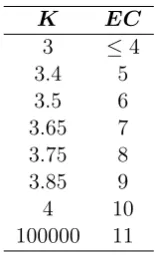
The factor, commonly known as the multiplier, is then defined according to Table 1. This allows supervisors to have a higher confidence when approving models and provides an incentive for risk analysts to create good models in order to reduce the capital requirements
2
Exceedances k factor
≤4 3
5 3.4
6 3.5
7 3.65 8 3.75 9 3.85
≥10 4
Table 1: Relation between the number of exceedances and the k factor.
(i.e. the capital charge) through lower multipliers.
Lastly, in order to avoid the need of sharp increases in the minimum required capital related with the high volatility of the market risk, especially when a sharp move in prices occurs, it is used the average of the last sixty days VaR in the calculation of the GRC.
In short, the previous rules can be translated into the following equation
GRC = max k× 1 60
59
X
i=0
V aR1,1%,t−i×
√
10, V aR1,1%,t×
√
10
!
(2)
In terms of the SRC the BCBS defines that it should be zero when regulators approve that the VaR model is capturing all the specific risk, otherwise it should be estimated according to the standardized method.
An important note about the Basel accords is that none of these measures are manda-tory, these are recommendations that are discussed by the committee, in order to improve risk management efficiency. The application of these measures depend on their adoption by the regulators in each country. Nonetheless, the first Basel accord and the 1995 Market Risk Amendment were adopted by more than 100 countries (Alexander, 2008) – including the Eurozone countries – which demonstrates the large influence of the BCBS.
Due to the effect of the 2007/2008 financial crisis the BCBS revised Basel II and published a new report in 2009 entitled “Revisions to the Basel II market risk framework”. The main reason for this was that the previous measures did not account for some key risks, e.g. default risk and migration risk.
In this report, some of the rules to use internal models were changed. FIs are now obliged to update their data once every month and they must compute, on a weekly basis, a stressed- VaR (sVaR) measure in order to verify how their model would react to a period of financial stress. This sVaR is also part of the GRC, and it is added to equation 2.
Regarding the SRC, for VaR models that have specific risk recognition it should now be added an IRC (Incremental Risk Charge) to the MRC, which is an estimate of the exposure to systematic and specific default, credit migration, credit spread and equity price risk in a period of 1 year and with a confidence level of 99.9%.
be considered the rules reported until the Basel Accords II, meaning that our model will optimize one part of the GRC (equation 2) and not the full amount as it is defined nowa-days.
2.2 Value-at-Risk
As it was stated above, the Value-at-Risk represents the loss that will not be exceeded with a certain confidence level (1−α) over a certain period of time (h) (Alexander, 2008). From
this it is easy to understand that the VaR is a statistic and it is related with a probability:
P(Xh <−V aRh,α) =α (3)
The popular use of this risk measure to address market risk is mainly due to its com-prehensibility and ability to be disaggregated and aggregated while taking into account the dependencies between the assets, allowing the determination of the origin of the risks in a portfolio. In order to estimate VaR it is necessary to define the values for the two pa-rametersαand h, the distribution of h-day returns (Xh) and the method used to estimate
the VaR.
The first two parameters have to be chosen according to the rules under the Basel II –α is equal to 1% and h is equal to 10 trading days. The return distribution will depend on the estimation method used. The choice of this method is the most important step in the development of the VaR model since it is one of the main drivers for its performance. In a study made by Beder (1995) the VaR was computed according to eight different methodologies for three portfolios and the results indicated eight significantly different values, varying in some cases by more than fourteen times in the same portfolio.
Alexander (2008) explores three main methods for VaR estimation: Parametric VaR, Historical Simulation and Monte Carlo Simulation. The Parametric VaR model is based on the assumption that the return distribution follows a certain parametric distribution, usually the Normal distribution. The historical simulation is a nonparametric method that uses the empirical distribution of the returns in a given sample. The Monte Carlo Simulation is a more advanced method that consists in using a statistic model to simulate the future returns, being at the same time extremely flexible but also more prone to risk model risk.
According to a survey made by Pérignon and Smith (2010), the most common method used by FIs is the historical simulation, choice that is not difficult to understand since it is the one that has the least assumptions and is easier to explain in case of failing.
In this paper the estimation method used is the Parametric Normal – assumes that the return distribution follows a normal distribution – due to its simplicity and easy compu-tation. Therefore the focus, from now on, will be on this method.
distributed) with a certain mean and standard-deviation (i.e. volatility):
Xh∼N(µh, σh) (4)
Both parameters are the forecasts of the future expected return and volatility over the following h-days. From this assumption it is easy to derive the formula for the VaR.
V aRh = Φ−1(1−α)×σh−µh (5)
whereΦ−1(·) is the quantile function for the standard normal random variable.
Alexander (2008) demonstrates that using an expected value (i.e. mean) equal to zero makes the computation of VaR easier and only has a big effect in its value when the risk horizon (h) is higher than one month. Thus, to simplify this equation, we will assume that the mean is equal to zero.
V aRh = Φ−1(1−α)×σh (6)
Now that the formula is derived there is one last concept to understand: scalling. Basel rules define that the 1-day VaR can be scalled in order to obtain the 10-day VaR. The purpose of this strategy is to avoid the use of a big sample when a 10-day VaR is estimated, since this would lead to a forecast of the parameters based in a considerable amount of past data.
This scalling is done by multiplying the 1-day VaR by the square root of time (in our case, 10 days). However, it is necessary to do an extra assumption to be able to use this rule: the arithmetic returns are approximately equal to the geometric returns.
When this rule is used it means that we are computing a dynamic VaR. This assumes that the portfolio is rebalanced every day, i.e. its value has to remain the same in the end of each trading day over the h-day horizon. This is why the Basel Accords states that the VaR must be computed on a daily basis.
Lastly, it is necessary to forecast the volatility to compute the VaR. This is another of the main drivers that are directly related with the performance of the model. Some of the most common methods, in ascending order of complexity, are the equally weighted variance, the EWMA (Exponentially Weighted Moving Average) and GARCH (Generalized Autoregressive Conditional Heteroscedasticity) models.
The difference between the equally weighted variance and the others is that the first is sensitive to the sample size, while the others are not, because the weight of an observation in the volatility estimation decays exponentially with the age of that observation. Due to this, it becomes a better method to estimate future values. For these reasons, the method that will be used in the empirical tests is the EWMA since it is the simplest method that gives good forecasts for the future variance.
The recursive equation of this method is the following (Alexander, 2008):
ˆ
According to this equation, the variance is computed in a recursive form and this is the reason for the smaller impact of past observations on the variance, as time passes. This can be observed in the next equation.
ˆ
σ2t = (1−λ)
∞
X
i=1
λi−1X12,t−i (8)
To apply this method it is necessary to give a value to the parameter λ, i.e. the
smoothing constant, in order to define the different weights that the most recent and older observations have in the future variance. In JPMorgan (1996) a calibration for this parameteris performed using the RMSE (Root Mean Square Error). The values achieved were 0.94, when considering daily data, and 0.97, for monthly data.
2.3 Dynamic Programming
Dynamic programming (DP) is used to do optimizations when a multi-stage decision prob-lem is addressed, i.e. the optimal decision depends on the current state.
The base for the DP model is Bellman’s principle of optimality (Bellman, 1954) that states that an optimal policy should always define the optimal decision to take considering all the previous decisions in order to maintain the final result in its optimal level.
Dynamic models are categorized depending on whether time, state space (S) and action space (X) are discrete or continuous (Miranda and Fackler, 2002). As it will be demon-strated later, the proposed optimization problem has a finite discrete space of states and an infinite continuous space of actions. However, in order to reduce the complexity of the problem, we will discretize the action variable, meaning that the correct model to use is one that is discrete in time, state and actions. The reason for this choice will be explained in Section 4.
The discrete model that will be used is the discrete Markov Decision Model. Its struc-ture is: in each periodtit is observed the current statestand, according to the
character-istics of that state, an action xt is taken by an agent, resulting in a reward f(xt, st) that
is directly related with the state and the action Miranda and Fackler, 2002). Given the decision, the agent will pass to the next statest+1 . This transition is deterministic, if the
next state can be determined just from knowing the current state of nature and action, otherwise it is stochastic. If it is stochastic, it is necessary to define a transition function
g(xt, st) that contains the probabilities of transitioning from one state to another.
Taking all of this into account it is now possible to derive the Value Function according to Bellman’s principle of optimality (Miranda and Fackler, 2002):
Vt(s) = max
x∈X(s)f(x, s) +δ
X
s′∈S
P s′ x, s
×Vt+1 s′, s∈S (9)
In the previous equation we have the reward functionf(x, s), a discount factorδ, the probability of transitioning to the next state P(s′
the value function of the next period Vt+1(s′). This equation reflects the maximization
problem that is: take an action x today in order to maximize today’s reward and the
discounted expected future rewards. To achieve the optimal policyx∗
(s), it is necessary to guarantee that, in each state, the decision maximizes the present and future rewards. This is achieved by using a recursion method, starting from the last period T until today. This equation is named Bellman’s
recursion equation (Miranda and Fackler, 2002).
According to the time horizon there are two possible types: finite and infinite horizons. If the horizon is finite it means that the last decision is taken at timeT. On the other hand,
an infinite horizon means that it is necessary to take a decision for an infinite number of time periods, therefore Bellman’s equation does not depend on time.
V (s) = max
x∈X(s)f(x, s) +δ
X
s′∈S
P s′ x, s
×Vt s′
, s∈S (10)
In this equation, Vt(s′) represents the value function considering the optimal results
forX(s)until that moment. The main difference between equations 9 and 10 is the time-dependence, i.e. while in equation 9 the purpose is to define an optimal decision for each point in time, in equation 10 the goal is to reach a single optimal policy that can be applied at every point in time.
The problem that will be presented later on will be solved as an infinite horizon problem therefore the next step is to describe the method that is commonly used to achieve the optimal policy in this type of problems.
Miranda and Fackler (2002) give some insight into the algorithms used to solve these problems using a computer software (e.g. MATLABTM
), nevertheless it is first necessary to transform equation 10 into matrix notation.
V1= max
x f(x) +δ×P(x)×V0 (11)
The value functionsV (s)andV (s′)are represented, respectively, by the vectorV 1 ∈Rn
and V0 ∈ Rn. The reward function is the vector f(x) ∈ Rn and the policy vector, that
contains the optimal actions to be taken at each state, is denoted by x ∈ Xn. Lastly, P(x) ∈ Rn×n represents the n-by-n probability transition matrix for a certain action.
Finally,nrepresents the number of possible states of nature.
After this, one can apply the specific algorithm in order to achieve the optimal value and policy function. In the case of the infinite horizon Markov decision model, the algorithm used is the Function Iteration Algorithm (Miranda and Fackler, 2002):
1. Define the state variablesS, action variableX, reward vector f(x), discount factor
δ, transition matrixP(x), termination condition τ, and an initial value forV0;
2. ComputeV1= maxxf(x) +δ×P(x)×V0;
4. If the termination criterion is satisfied: x→x∗.Else, update V
0 to V1 and return to
step 2.
3
Literature Review
Since the introduction of Value-at-Risk, research has focused on Value-at-Risk potential uses and on how to accurately estimate it.
Studies have been produced where the VaR measure is used as a substitute for the variance in portfolio optimization problems. A recent study conducted by Deng et al. (2013) combines the VaR concept with the Sharpe Ratio – amount of expected return an investor gains for each aditional unit of risk that it takes – in order to optimize the value of the portfolio.
Other studies on this subject (e.g. Künzi-Bay and Mayer, 2006; Mansini et al., 2007; Lim et al., 2010; and Ogryczak and Sliwiński, 2011) used the CVaR (Conditional Value-at-Risk) – measures the risk of extreme losses calculating a weighted average of the expected losses that go beyond the VaR estimate – instead of the VaR to optimize the return on portfolios using Linear Programming models.
However, there are few studies related with the regulatory context of the VaR, namely optimization strategies for the market risk charge. Ahn et al. (1999) studied a method that could be used to find a put option that minimizes the VaR, considering a maximum hedging cost. This was performed by modeling a function that computes the optimal options’ strike price taking into account the underlying asset’s value, the mean and volatility of its return, the risk-free rate and the VaR hedging period. One of the main conclusions in this paper is that this optimal strategy can reduce the VaR by 45% comparing it with a normal strategy of using at-the-money options, in an equity portfolio, at the same time that it can reduce the cost of the strategy by up to 80%. Deelstra et al. (2007) studied the optimal risk management strategy for a portfolio of bonds and consisted in determining the optimal strike price of a put option that would minimize the VaR for a certain hedging cost.
Although these methods were proved to be good strategies to reduce VaR (hence reduc-ing the capital charges), they focus in the use of other financial products and in portfolio management to achieve certain VaR objectives (i.e. its minimization).
What if there exists a method to optimize VaR without the need to incur in addi-tional costs or in increasing the exposure to financial assets? McAleer (2009) addresses this question. In this paper, some guidelines are given about the improvements that can be made in VaR models in order to create better risk monitoring strategies and achieve superior forecasts for the VaR. The purpose is to manage the excessive risk taking, that is a characteristic of conservative financial institutions, and achieve an optimal VaR measure following the Basel rules.
to forecast VaR (parametric, semiparametric and nonparametric models).
Altough the presented methodology is of important use in the creation of a VaR model, it only gives an optimal strategy for risk monitoring and does not truly explores strategies to optimize the daily capital charges. Moreover, this study raises one question: Is disclosing a perfect estimation for the VaR the best strategy to optimize the capital charge?
The first answer to this question came in McAleer et al. (2010). This paper discussed the hypothesis that FIs could manage the number of exceedances that they are allowed to have according to the Basel Accords (10 exceedances), in order to optimize the daily capital charge. To achieve this purpose, they created a function named DYLES (Dynamic Learning Strategy) that was based in the trade- off between the expected number of exceedances and the expected capital requirements.
This function gives the percentage of the forecasted VaR that should be disclosed, taking into account the number of exceedances that the FI had since the beginning of the regulatory period and the number of exceedances recorded in the last 25 days. The foundations of this function are related with the premise that risk managers are conservative when the number of exceedances is high and aggressive when this number is small or zero. This method tries to optimize the capital charges by doing a policy that manages the Basel rules, taking advantage of them. The authors tested this theory and reached to the conclusion that using DYLES reduces the daily capital charges by up to 14.3% when compared with the RiskMetrics Policy.
While this seems to be a great tool to optimize the capital requirements taking into account the Basel rules, there is still some inconvenients with it. The function has three parameters for which the value is a subjective choice, meaning that the performance of the function has some dependence on those parameters’ values.
The authors give some suggestions about the numerical intervals for the parameters, however to achieve the perfect model it is necessary to do a callibration that consists in computing the results for DYLES using all the possible parameter combinations and then choosing the one that has the lowest number of exceedances and average capital requirements. Thus, this process is time consuming and makes the model less user friendly. The second incovenient is that it is an ad-hoc strategy, meaning that each strategy depends on the specific portfolio and does not have a general application. It is also im-portant to point out that the authors only did an in-sample test, which means that the effectiveness of this model in a real life situation is unknown.
Following this thought, we propose to present an alternative method to do this opti-mization. Based in the same principle as DYLES, this paper consists in creating a model that optimizes the daily capital charge through the use of DP.
the current regulatory period (EC); and multiplier that is currently in use (K). The focus is in the 1-day VaR because the exceedances are defined according to its value, and it is the only one that is in the control of the risk analyst (see equation 2).
The advantages of this model are: all the parameters are defined; in each state of nature there is an optimal decision; and the optimal policy strategy can be applied to any portfolio. The main contribute of this study for the financial literature is to demonstrate that, taking into account the market risk framework that is associated with the definition of the capital charge, the best strategy to optimize the regulatory capital may not be through the disclosure of a precise estimate for the 1-day VaR.
4
Optimization Model
The goal of this paper, as it was mentioned in the previous section, is to create a model that allows the optimization of the market risk charge when the VaR method is used. It consists of maximizing a value function, through the use of DP, in order to obtain an optimal policy function that provides the optimal decision that an agent should take regarding the reported VaR.
The policy function defines the percentage of the estimated VaR that should be reported in order to optimize the daily capital charge, taking into account all the future effects of today’s decision, in particular the likelihood of future exceedances and the future value of the multiplierK.
The action space (X) corresponds to all percentages of the estimated VaR that can be
reported, which can be any value from 0 to infinity, therefore making the action space con-tinuous. However, we tested the possibility of solving the dynamic programming problem with a continuous action space and reached the conclusion that it was computationally intractable. Therefore we decided to discretize the action space, maintaining a wide range of possibilities, ranging from 0.001 to 3, in steps of 0.001.
X ={0.001,0.002,0.003, . . . ,3} (12)
This means that the lowest value that can be reported is 0.1% and the highest value is 300% of the estimated 1-day VaR.
The choice of the percentage to report will depend on three state variables: time re-maining for the regulator to do the backtesting and review the multiplier (T toB); multiplier
that is currently in use (K) and the number of exceedances that were recorded until now
(EC). All these state variables are discrete and the set of possible values are as follows:
T toB={1,2,3, . . . ,250} (13)
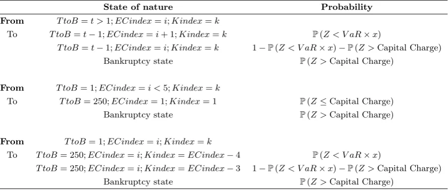
K ={3,3.4,3.5,3.65,3.75,3.85,4,100000} (14)
K EC
3 ≤4
[image:15.595.258.336.82.210.2]3.4 5 3.5 6 3.65 7 3.75 8 3.85 9 4 10 100000 11
Table 2: Relation between the number of exceedances at the end of the year and the multiplier.
The values ofT toB are derived from the Basel Accords, where it is defined that, to do the backtesting analysis, the regulator must use data from the last 250 days to evaluate the performance of the risk model (Basel Committee on Banking Supervison, 1995). In terms of the EC, the Basel Accords state that, when it is higher than 10, the most probable consequence is the obligation to use the standardized method instead of using the internal model. Therefore we restricted theEC variable to a maximum value of 11 since we assume
that the agent pretends, at all costs, to use the internal model for an infinite horizon. The
K variable includes all the multipliers that are in the Basel accords plus an additional one (100000). The purpose of this multiplier will be explained later. Table 2 relates the multiplier with theEC at the end of each 250-day period.
For any combination of these three states, the optimal policy function gives the decision that should be taken in order to minimize the daily capital charge. This type of DP problem is known as infinite horizon Markov decision model and is solved with the function iteration algorithm (Miranda and Fackler, 2002) introduced in Subsection 2.3.
4.1 Methodology
In this subsection we are going to follow all the steps mentioned in the Subsection 2.3, in order to derive the Bellman’s equation and apply the Function Iteration Algorithm.
First, it is necessary to change the notation of K and EC variables. For a better
connection between this explanation and the program code, the state variableK andEC
will be substituted by Kindex and ECindex, respectively, which represent the index of each variable. For example, Kindex = 2 corresponds to the second smallest value of K,
that is, 3.4, andECindex= 1 corresponds to the smallest value of EC, that is, 0.
Kindex={1,2,3,4,5,6,7,8} (16)
ECindex={1,2,3,4,5,6,7,8,9,10,11,12} (17)
average will be ignored; it is assumed that the capital charges will always be the 10-day VaR multiplied by the multiplier K; and the capital charge is equal to the GRC, meaning that we assume that the risk model as specific risk recognition (SRC=0).
f(x, T toB, EC, K) =−x×K×V aR1,1%×√10 (18)
The Breakdown of this equation is the following: V aR1,1%× √
10 – represents the 10-day VaR that is in compliance with the Basel Accords; K is the multiplier for the current period;xis the percentage of the VaR to be reported (the action variable).
As one can see, this function has a negative sign because we are maximizing the FI’s profit, meaning that the capital charge has a negative impact in the function.
Now that this was explained, it is possible to justify the additional multiplier: 100000. In the definition of the EC variable we limited the number of exceedances up to 11
be-cause otherwise we would have 251 possible values for the ECindex instead of 12. This would unnecessarily increase the dimensionality and complexity of the problem, making it intractable to reach a solution. To prevent this, we created a new multiplier (100000), associated with anECindex equal to 12, that represents the transition to a state with a very high cost (equation 19 below). With this mechanism we assure that the agent will do whatever it takes to prevent the transition to this state, which will probably result in disclosing the highest possible percentage of the 1-day VaR (i.e. 300%). Note that the value of this multiplier is only used to determine when the transition to this state occurs, meaning that it does not have an application in the general reward function (equation 18) as it can be seen in equation 19.
f(x, T toB, EC, K) =
−x×K×V aR1,1%× √
10 ifKindex≤7
−5000000000 ifKindex= 8
(19)
To be able to apply the Function Iteration algorithm it is essential to translate this function into matrix notation. This is done by creating a reward vector named RewFun with 250 × 8 × 12 = 24,000 elements that represent the total number of possible state
combinations (achieved by multiplying the total number of elements of each state variable). Lastly, it is necessary to construct the Transition Functiong(x, T toB, EC, K)that will define how the transitions occur between states of nature. In this problem, one can see that the state variables are not independent because the multiplier (K) depends on the EC when T toB is equal to 1. The reason for this is that the multiplier must be reviewed at the end of each 250-day period in accordance with the EC variable. Due to this, it
is necessary to implement a transition function with all the possible state combinations instead of doing one function for each state variable. Next we discuss the main ideas behind these transitions.
fact that at this time the backtesting is performed and the number of periods for the next backtesting is reset to 250 days.
The transition betweenKindex states is, most of the times, deterministic. Whenever T toB > 1 no backtesting is performed, which means that the multiplier is not revised. Hence, the state Kindex remains unchanged. But, at T toB = 1, on the eve of perform-ing the next backtest process, the state Kindex is updated, reflecting the results of the
backtesting process and the Basel rules outlined in Table 2. In this scenario, the transition is stochastic, since it depends on the state ECindex (how many exceedances were
accu-mulated up to T toB = 1) and whether there was an exceedance in the transition to the next period, which is a random event. The new stateKindexis determined as follows: for
ECindex <5(less than 4 exceedances up to the eve of the backtesting procedure)Kindex
transitions to 1 regardless of whether an exceedance is recorded in the transition to the next period; for 5≤ECindex <12, Kindextransitions to the current value of ECindex
− 4 if no exceedance is recorded and, otherwise, to the current value of ECindex − 3;
and forECindex= 12,Kindextransitions to 8, the catastrophic scenario that the agent wants to avoid at all costs.
Finally, the transition betweenECindexstates is, most of the times, stochastic.
When-ever T toB > 1, there is some probability that an exceedance is recorded (portfolio loss is higher than the reported VaR), in which case the ECindex state transitions fromi to
i+ 1, and some probability that an exceedance is not recorded, in which case theEC state
remains unchanged. At T toB = 1 the transition is deterministic, since the exceedance count is reset when entering the new backtesting. HenceECindextransitions to 1.
On top of this, there is always a possibility of falling into bankruptcy if the portfolio loss is larger than the capital charge set based on the reported VaR. This possibility, and its associated high costs, effectively put a limit to extreme levels of VaR underreporting. In that case, and regardless of the current state of nature, the transition is made to a state of nature withT toB= 250,ECindex= 12andKindex= 8which, according to equation 19, is the state with a very large cost that reflect the bankruptcy cost. Table 3 summarizes the different transition scenarios and their probabilities.
To compute the probabilities associated with each scenario we assumed that returns follow a standard normal distribution (mean zero and standard deviation of one). These probabilities of transition between states are then represented by a 24,000 by 24,000 matrix named TrMat.
At this point we have all the essential tools to derive the value function that we want to maximize. This function is equation 11 that was introduced in subsection 2.3 (DP), with an adjustment for our notation.
V1 = max
x RewF un(x) +δ×T rM at(x)×V0
To initiate the algorithm it is still necessary to define the value for the parameter
State of nature Probability
From T toB=t >1;ECindex=i;Kindex=k
To T toB=t−1;ECindex=i+ 1;Kindex=k P(Z < V aR×x)
T toB=t−1;ECindex=i;Kindex=k 1−P(Z < V aR×x)−P(Z >Capital Charge) Bankruptcy state P(Z >Capital Charge)
From T toB= 1;ECindex=i <5;Kindex=k
To T toB= 250;ECindex= 1;Kindex= 1 P(Z ≤Capital Charge)
Bankruptcy state P(Z >Capital Charge)
From T toB= 1;ECindex=i;Kindex=k
To T toB= 250;ECindex=i;Kindex=ECindex−4 P(Z < V aR×x)
[image:18.595.91.543.85.277.2]T toB= 250;ECindex=i;Kindex=ECindex−3 1−P(Z < V aR×x)−P(Z >Capital Charge) Bankruptcy state P(Z >Capital Charge)
Table 3: Transitions that occur in each scenario and the equations used to compute their associated probabilities (where Z represents a standard normal random variable and x
represents the action variable).
current decision, the terminal conditionτ, and an initial value for the value function,V0. We defined a yearly discount factor of 0.9, meaning that the daily discount factor is approximately 0.99957865.3
Regarding the terminal condition, it is decided that the norm of the difference betweenV0 andV1 should be close to 0.001 in order to consider the policy functionx as the optimal one (in the case of our model, this value was 0.0013).
Due to the complexity of this problem, it is essential to start with a reasonable guess for the initial value ofV0 in order to reduce the number of iterations necessary to achieve the terminal condition (and the optimal solution). Thus, the initial value for V0 will be a
24,000 by 1 vector, that was obtained from the solution of a similar optimization problem, but with a smaller number of possible actions (300 instead of 3,000).
4.2 Model vs Reality
After modeling the problem, it is necessary to understand the differences between our model and the real life problem. These differences will be important, later on, in the identification of the limitations of this study.
One of the most important assumptions in the construction of the model is related with the distribution of returns. To simplify the computations, we assumed that the distribution and its parameters (expected return and volatility) are known with 100% certain.
As mentioned in Subsection 2.2, using a value of zero for the expected return is a good proxy and does not have a material impact in the results. The biggest problem lies in the volatility since, in reality, it is unlikely to predict the true value for the future volatility. Usually one works with estimates that can either under or overestimate the true value of the volatility. In our case, the scenario of underestimation of the true volatility is the one
3
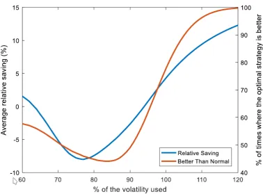
that represents a real danger. In that scenario, the underestimation of the volatility itself will be enough to generate too many exceedances. If, on top of that, the agent pursues the optimal VaR disclosing policy that is derived under the assumption that his volatility estimate is correct, he will tend to underreport and underestimate the VaR. That will inevitably lead to a fast accumulation of exceedances from which it is impossible to recover and that, next year, will result in a high multiplier being set by the regulator and thus high capital charges. The scenario of volatility overestimation is more benign. The agent will see too few exceedances being generated despite his VaR underreporting, but the only implication is that we will have more freedom to keep underreporting the VaR. These scenarios and their consequences for the application of the optimal VaR reporting policy will be tested later on in a Monte Carlo Simulation in order to investigate the extent to which the performance of the optimal policy is sensitive to the assumption that the true volatility is known.
The next assumption is related with the reward function. According to the 1995 Market Risk Ammendment (Basel Committee on Banking Supervison, 1995), the GRC is defined as the maximum between (a) the average of the 1-day VaR forecasted for the last sixty days multiplied by the square root of time and byK and (b) the last forecast for the 1-day
VaR multiplied by the square root of time. However, in the reward function defined in equation 18 and 19, the maximization and the average are ignored, and it is assumed that the capital charge is always the reported 1-day VaR multiplied by the square root of time and by the multiplierK.
Ignoring the maximization does not make any effect in the results since, assuming a constant portfolio, it is very unlikely to have the last VaR estimate to exceedK times the
average of the last sixty VaR’s becauseK has a value between 3 and 4. Therefore the most important difference between the model and the real life problem is the averaging of the last sixty VaR’s, which is omitted in the model.
This average is important to avoid a manipulation of the reported VaR, however it is hard to implement in an optimization problem and if implemented it dramatically increases its complexity, since we would have an additional 59 state variables (the VaR reported in the previous 59 days), making it intractable.
Considering this, a possible solution is to ignore the average and only consider the last estimated VaR. We concluded that this does not result in the most optimized strategy but it gives a quite good approximation for it. The following demonstration proves this. For simplification, assume that there is no uncertainty, so we can drop expectations. The dynamic programming problem we solved is equivalent to minimizing the present value of the capital charges.
P V (GRC) =
∞
X
t=0
δtGRCt (20)
The formula we consider for the GRC is
In reality, the formula for GRC is (dropping the maximization):
GRCtreal=k√10 1 60
59
X
i=0
xt−iV aRt−i (22)
If the impact of the choice variable, xt, in P V (GRC) is similar for both formulations of
GRCt(real and modeled), then the approximation has a small impact
∂P V GRCtmod
∂xt
= ∂
P∞
t=0δtk √
10xtV aRt
∂xt
=δtk√10V aRt (23)
In turn,
∂P V GRCreal t
∂xt
= ∂
P∞
t=0δtk √
10601 P59
i=0xt−iV aRt−i
∂xt
=k√10 1 60
59
X
i=0
V aRtδt+i
=δtk√10V aRt
1 60 59 X i=0 δi
≈δtk√10V aRt (24)
since 1 60 59 X i=0
δi ≈1 (25)
as long asδ is close to 1. In our case δ= 0.99957865 and so4
1 60
59
X
i=0
δi= 0.9877≈1 (26)
The last assumption is related to the Basel Accords. As it was stated in Subsection 2.1, our optimization model is in accordance with the rules introduced until Basel Accords II, and does not take into account the changes made by the revisions to the market risk framework published in 2009 (Basel Committee on Banking Supervison, 2009). One of the impacts that this has in the model is related with the probability of default, which is overestimated in the model. This happens because with the new standards the GRC would incorporate a new element – sVaR – meaning that the daily capital charge would be higher than the value considered by the model. On the other hand, not considering the sVaR means that our model only optimizes part of the capital charge, i.e. only the one related with the VaR.
Nevertheless, this does not invalidate the use of our model (to optimize the part related
4
with VaR) since, in the worst case, the effect of this change in the GRC would probably be a policy function where extreme underreporting is more likely to occur, especially when EC is low and in the last days of the 250-day cycle, due to lower probability of default.
4.3 Optimal Policy Function
In this subsection we are going to present the results of the optimization model. These represent the percentage of the estimated 1-day VaR that should be reported according to the three state variables: time remaining for backtesting (T toB), number of exceedances so far (EC) and multiplier in use (K). This will be referred, from now on, as the optimal policy.
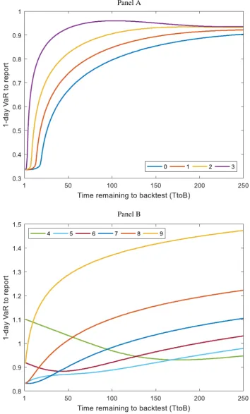
Figure 1 illustrates the percentage of the estimated 1-day VaR that should be reported for each point in time when the multiplier variableK is 3, which is divided in two panels according to the number of the EC variable. Thus, in the vertical axis one can find the
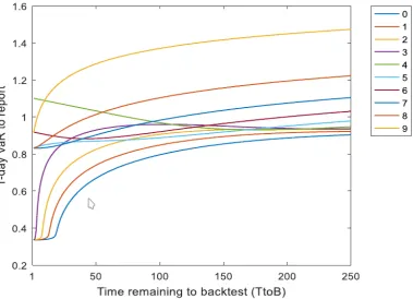
action variable (that can range between 0.01% and 300%) and in the horizontal axis one of the state variables –T toB (ranges between 1 and 250). Each line represents the different decisions that should be taken according to the value of the exceedance count variable (EC) at that time, e.g. if the current number of exceedances is equal to 5, one should find the optimal decision in the lighter blue line in panel B. Figure 2 shows all the lines of the two panels of Figure 1 in one figure.
The careful reader may have noticed that in both Figures 1 and 2 it is not included the series for the EC equal to 10 and 11. These two will not be presented here because
the optimal decision is always the same: report 300% when the EC is equal to 10 and
report 0.1% when theEC is equal to 11. This happens for a simple reason: if in any day, during the 250- day period, a portfolio records the 10th exceedance, it means that an extra exceedance will result in a transition to a state that we considered in the formulation of the model as a state with big consequences (e.g. the obligation to use the standardized method instead of the internal models) – referred, from now on, as the worst case scenario. Assuming that the agent does not want to face these consequences, he will do whatever it takes to avoid the extra exceedance, and the only decision that has the highest probability of not having an exceedance is reporting the maximum possible percentage of the VaR, 300%.
In the opposite case, when the EC is equal to 11 it means that this extra exceedance already occurred, therefore there is nothing that the agent can do to avoid these conse-quences, and for this reason the percentage to report is the lowest possible (0.01%). In other words, the damage is done.
Figure 2: Optimal policy function for all the number of exceedances when the multiplier
K is equal to 3.
EC 0 1 2 3 4 5 6 7 8 9
[image:23.595.111.491.86.360.2]Mean 0.7655 0.8118 0.8634 0.9190 0.9771 0.9083 0.9476 0.9930 1.1029 1.3611 Median 0.8305 0.8765 0.9230 0.9410 0.9470 0.9035 0.9435 1.0125 1.1335 1.3965
Table 4: Statistical analysis of the optimal policy.
50 days of the last 5 series is that the agent has more factors to take into account when choosing the optimal decision to take, since the goal of the 4 exceedances was not attained. This difference will be analyzed later on.
In the series for the 4th exceedance, the behavior is different because this is the max-imum number of exceedances that an agent can have in order to maintain the base mul-tiplier. As one can see, the percentage to disclose increases as the time to backtesting decreases, being the only series that has an increasing trend, ranging from 94.7% to 110%. This effort is made in order to avoid another exceedance that would lead to a multiplier higher than the base value (3) in the future. It is also important to notice that, when the barrier of the 4 exceedances is exceeded, this effort decreases, mostly due to the conse-quence of having a multiplier higher than the base value in the future (which translates in higher capital charges and lower long- term benefits).
confirms the reasoning used on the previous paragraph related with the series for anEC
equal to 4, by showing that the incentives to avoid an extra exceedance decrease after overcoming the barrier of 4 exceedances. From the 7th exceedance onwards, this effort is again high, reaching values higher than 100% when the worst case scenario is approaching. Looking at the average of the whole series (0.9650), we conclude that, on average, it is better to disclose a lower 1-day VaR than the estimated one, i.e. to underreport. This is a natural conclusion because our model is designed in order to achieve 4 exceedances, objective that is attained through the underreporting of the 1-day VaR. If the estimated VaR is reported truthfully (i.e. no under nor overreporting), then on average there will be only 2.5 exceedances in a year. This leaves room to underreport and reap the short term benefit of lower capital charges without incurring in the cost of larger long term capital charges due to larger multipliers as consequence of accumulating more than 4 exceedances in a 250-day period.
Next we go into detail for each series. In the first three series (EC equal to 0, 1 and
2), there is a decreasing trend, i.e. the first percentage to report, when T toB is equal to 250, is, respectively, 90.4%, 92.2% and 93.3%, and after that, these values decrease until they both reach 33.6% when T toB is equal to 1. This behavior was expected since, in
the beginning of the 250-day cycle, the agent is more risk averse due to the possibility of incurring in early exceedances that may accumulate to more than 4 by the end of the cycle, and, as time passes, this risk becomes smaller and the percentage to report decrease.
When theEC is equal to 3 (fourth series), the trend is also in general a downward one, although there is a slight increase between the 249 th and 92nd day to the next backtesting, going from 0.936 to 0.96. This is explained by the fact that the portfolio is 1 exceedance away from the 4th, i.e. the maximum value for theEC variable that guarantees the base multiplier, and it is related with the formulation of the optimization model. Since the goal is to optimize the present value of the capital charge, there are two factors that drive the optimal decision: report a lower percentage of the 1-day VaR to reduce the capital charge in the present (short-term benefits); or report a higher percentage to avoid an increase of the multiplier and benefit from this saving in the future (long-term benefits). To achieve an optimal model it is necessary to balance these two factors (referred from now on as “balancing factors”).
Considering this, in the first 157 days the predominant factor is the long-term benefits of having the base multiplier in the next regulatory period (hence there is an increase in the percentage to report), whereas after this, since the end of the period is approaching and the likelihood of incurring in two more exceedances reduces, the short-term benefits seem to gain the lead as the predominant factor and the percentage to report decreases.
The next series (EC equal to 4) is the only one with an increasing trend, explained
capital charges in the present and, following this, it seems to be better to report a higher percentage of the estimated VaR to benefit from a smaller multiplier in the future (in this case, the base multiplier).
Another possible explanation for this type of behavior (mix between decreasing and increasing trend) is related with the value of the EC variable in the early days. If, for
example, an agent records 4 exceedances too quickly, it will be difficult to maintain this number until the end of the period, thus there is no incentive to be conservative and disclose an higher percentage of the estimated 1-day VaR (decreasing trend). However, as time passes, if this extra exceedance does not materialize, the agent will try to avoid it by increasing the percentage to report, in order to guarantee the smaller multiplier in the next period (increasing trend). This reasoning applies to all the series that show this type of behavior.
From the 4th exceedance on, every additional exceedance results in an increase of the multiplier up to the 11th exceedance, which represents the transition in the future to the worst case scenario. Hence, the balancing factors will also drive the trend of the next series.
For an EC equal to 5, 7, 8 and 9, one can notice that the curves have a decreasing
trend and represent a higher risk aversion – the smallest percentage of the 1-day VaR to report is 83.1%. Also, for most of the time, the curves for the 7th, 8th and 9th exceedance are above 100%, which is due to the proximity to the worst case scenario (reaching 11 exceedances). Nevertheless, there is a curious observation when comparing the series for an EC equal to 5 and 7: in the last 30 days the values are higher in the former. The expectation for this would have been a persistence of higher values for anEC equal to 7.
This different behavior can be explained with the effect of a future higher multiplier in the scenario where theEC is equal to 7 (3.65) compared with the scenario of anEC equal to 5 (3.4), meaning that the short-term benefits have an higher impact in the agent’s decision – report a lower percentage to increase current savings, instead of a higher percentage to reduce future costs (the damage in the future multiplier is already done).
Considering the series for an EC equal to 6, one can observe a similar scenario to
the series for an EC of 4: a decreasing trend until the last 48 days, and after that, an increasing trend. Like in that case, this change in the trend is due to the effect of the balancing factors because, following the increase of 0.4 in the base multiplier –EC equal
to 5 – the second highest increase in the multiplier (0.15) occurs when theEC, in the end of the regulatory period, is equal to 7. Therefore in the first 202 days the predominant effect is the saving in the current capital charges (short-term benefits), while in the last 48 days it is the long-term benefits derived from the 0.15 saving in the future multiplier that leads to higher percentages to disclose.
Figure 3: Evolution of the optimal decision as a function of the number of exceedances for the same day.
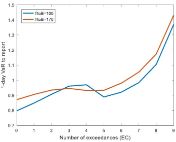
Following the blue line (T toB equal to 100), one can see that the percentage to report increases until the 4 th exceedance and then it falls from 0.969 to 0.888, followed by an increase until the highest possible number of exceedances. This decrease that occurs when theECis equal to 5 is due to the increase of 0.4 in the base multiplier (the highest possible increase, compared with 0.1 and 0.15 for additional exceedances), which translates into lower future savings and consequently lower long-term benefits. Since this possible saving in the multiplier was not achieved, the incentives to avoid another exceedance decrease and the current savings (short-term benefits, benefit today from reporting a lower VaR) seem to have a higher impact in the optimization strategy. For the curve where T toB is 170 (red line), this fall occurs in the transition from the 3rd to the 4th exceedance, which is even more surprising since the change in the multiplier occurs only in the 5th exceedance. This seems to be an effect from the balance between having current savings in the capital charge (report smaller percentages of VaR) and benefit from these savings in the future (report higher percentages to assure a small multiplier in the future).
Finally, it is important to remind that the analysis of the optimal policy function performed in this subsection was based on the scenario where the multiplierKis equal to 3.
However, all the qualitative results obtained from this analysis stand for different values of
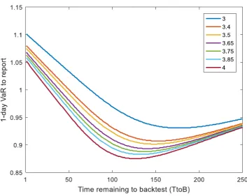
Figure 4: Optimal policy function for a number of exceedances (EC) of 4 considering different multipliers (K variable).
more conservatively is independent of the current multiplier (it is only a function of future multipliers), a higher multiplier will then increase the incentive to underreport the VaR. This can be clearly seen in Figure 4, which plots the optimal percentage of the observed VaR to report as a function ofT toB for all different multipliers whenEC is 4. For other values of EC, the conclusion is the same. Notice that the distance between each line is roughly
proportional to the difference in the values of the corresponding multipliers, reflecting the fact that the more the multiplier increases, the more the incentive to underreport increases. In Appendix A one can find the figures for the optimal policy considering the other multipliers.
In general, these results seem to be, more or less, consistent with the principle of DYLES (McAleer et al., 2010): risk managers are conservative (report higher percentages) when the number of exceedances is high and aggressive (report lower percentages) when this number is small.
5
Monte Carlo Simulation
In this section, we perform a Monte Carlo simulation in order to obtain simulated portfolio returns and evaluate the performance of the optimal policy presented in the previous section.
To do this process, we use MATLABTM
’s random number generator (RND) to generate returns from a normal distribution – using the inverse CDF of the normal – with an expected return of 0 and a certain standard deviation. Considering this, we will simulate the returns based on the following equation:
r= Φ−1(RN D), r∼N(0, σ) (27)
The base value for the 1-day standard deviation (σ) is 1.7%, which we considered to be reasonable for a standard portfolio. To compute the VaR we use the same Parametric Normal Method that was considered when solving for the optimal strategy.
Two scenarios are going to be simulated. In the first one, labeled Normal Strategy scenario, it is always reported 100% of the estimated VaR. In the second one, labeled Optimal Strategy scenario, the percentage to report is defined according to the optimal policy. To limit the possible number of exceedances to 11 (like in the optimization model), when theECis equal to 10 in both scenarios, it is reported 300% of the VaR (i.e. the same
value defined by the optimal strategy). Another way of understanding this assumption is that, in both cases, going to the 11th exceedance means transitioning to the worst case scenario (mentioned in the previous section) which is something that the agent wants to avoid, regardless of the strategy in use. Due to this, the agent will always report a high value when the number of exceedances is equal to 10, in order to almost surely guarantee that the 11th exceedance is avoided.
It is also incorporated a mechanism for bankruptcy detection, i.e. if the loss in a certain day is higher than the daily capital charge it is assumed that the institution defaults, which brings that specific simulation to an end.
5.1 Normal Simulation
The first simulation that we will perform consists of 100,000 simulations of a period of 30 years, considering that each year has 250 business days. The value defined previously for the standard deviation will also be used to calculate the daily VaR according to equation 6. The multiplier used in the first year of each simulation is always the base value (3).
We start by analyzing the daily capital charge variable in order to verify if the optimal strategy delivers lower values than the normal strategy, and then we look closely at the other variables to confirm whether their behavior is in line with our expectations regarding the optimization model.
Figure 5: Distribution of the average daily capital charge across simulations, and the respective cumulative frequencies (right axis).
representing the cumulative frequencies.
From the analysis of Figure 5, one can notice that there is a clear separation between the optimal and the normal strategy. The values for the optimal strategy seem to be concentrated between 35% and 38% while, in the normal strategy, these are concentrated around 38% and 39%, clearly pointing out to a better performance of the optimal strategy. The line for the cumulative frequencies proves this, since with the optimal strategy the capital charge is below 38% in, approximately, 100% of the simulations, whereas, with the normal strategy, this only happens in, approximately, 40% of the simulations. Taking this into account, it is clear that the optimal strategy delivers lower values for the daily capital charge in almost all simulations.
Table 5 complements Figure 5 by analyzing the annual average of the daily capital charge with 5 important statistics computed in two different ways: (1) by averaging the statistics calculated in each simulation (i.e. in each 30-year period); and (2) by computing the statistic on all the data (i.e. the results of all simulations).
As expected from the analysis of Figure 5, Table 5 confirms the better performance of the optimal strategy in terms of the capital charge since, with the analysis of the mean, it is easy to see that this strategy offers a lower capital charge.
Capital Charge
Mean Median Max. Min. Std. Dev. Optimal Strategy
Average of statistic 36.47% 35.45% 43.12% 32.51% 2.94% Statistic of simulation 36.47% 35.34% 68.54% 31.20% 3.00%
Normal Strategy
Average of statistic 38.12% 37.52% 44.03% 37.52% 1.72% Statistic of simulation 38.12% 37.52% 70.24% 37.52% 1.82%
Table 5: Average of the statistics computed for the annual average of the daily capital charge in each simulation (30-year period) and the statistics for the global simulation.
Mean Median Max. Min. Std. Dev. % Optimal better than Normal 77.81% 76.67% 100.00% 36.67% 8.55%
Table 6: Statistical analysis of the variable: percentage of times, in a 30-year period (each simulation), where the optimal strategy outperforms the normal strategy.
to the risk associated with the optimal strategy (i.e. the risk to report a higher value than the estimated 1-day VaR) that is translated in a higher standard deviation. This can be observed clearly in Figure 5, since the values for the optimal strategy are more dispersed. In the case of the maximum and minimum (average and global), the results confirm the outperformance of the optimal strategy as both statistics deliver lower values considering this strategy.
As the careful reader may have noticed, the value for the global maximum, in both strategies, is around 70%, which is a value that stands out from the others. The reason for such a high value is the trigger mechanism related with a number of exceedances of 10 – report 300% of the estimated 1-day VaR in both policies. From this we can conclude that, when the market conditions are adverse, the disclosure of the estimated 1- day VaR (normal strategy) does not necessarily lead to better results.
Table 6 shows the analysis of the percentage of times, in each simulation, where the optimal policy delivers lower values for the capital charge. This table shows that the optimal strategy outperforms, on average, the normal strategy in 78% of the times, which is a very good result taking into account the risks associated with this strategy.
Looking at the maximum and minimum, it can be noticed a big range between them. On one hand, we have simulations where the optimal policy is always better (100%) during the 30-year period and, on the other hand, simulations where this value goes as low as 36.67%. Once again, this behavior can be explained by the risk associated with the optimal strategy that is translated in the standard deviation of this variable (8.55%).
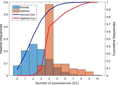
Figure 6: Distribution of the EC variable, in the end of the period, across the various simulations, and the respective cumulative frequencies (right axis).
Next, we move on to the analysis of the number of exceedances (EC) and multiplier (K) variables. In the formulation of the optimization problem, it was considered that
the objective of the optimal policy would be to take advantage of the Basel rules by managing the number of exceedances, in order to maintain the base multiplier (maximum of 4 exceedances). The purpose of the next analysis is to show if this event is true when this policy is applied.
As one can see in Figure 6, the distribution of the EC variable is significantly differ-ent for each strategy. In the Normal Strategy, the variable seems to follow a lognormal distribution with a mode equal to 2, while in the Optimal Strategy the variable is clearly concentrated in the 4th exceedance – the maximum number of exceedances that does not result in the increase of the base multiplier. This proves that the optimal policy is taking advantage of the Basel rules, regarding the exceedances, because there is a big discrepancy between the numbers of years that end with 4 exceedances (58%) and also because the minimum relevant number of exceedances, in the optimal strategy, is 3 (vs 0 in the normal strategy).