2009
Semi-supervised User Geolocation via Graph Convolutional Networks
Afshin Rahimi Trevor Cohn Timothy Baldwin
School of Computing and Information Systems The University of Melbourne
{t.cohn,tbaldwin}@unimelb.edu.au
Abstract
Social media user geolocation is vital to many applications such as event detection. In this paper, we proposeGCN, a multiview geolocation model based on Graph Con-volutional Networks, that uses both text
and network context. We compareGCN
to the state-of-the-art, and to two base-lines we propose, and show that our model achieves or is competitive with the state-of-the-art over three benchmark geoloca-tion datasets when sufficient supervision is available. We also evaluateGCNunder a minimal supervision scenario, and show it outperforms baselines. We find that high-way network gates are essential for control-ling the amount of useful neighbourhood expansion inGCN.
1 Introduction
User geolocation, the task of identifying the “home” location of a user, is an integral component of many applications ranging from public health monitor-ing (Paul and Dredze, 2011; Chon et al., 2015;
Yepes et al., 2015) and regional studies of senti-ment, to real-time emergency awareness systems (De Longueville et al.,2009;Sakaki et al.,2010), which use social media as an implicit information resource about people.
Social media services such as Twitter rely on IP addresses, WiFi footprints, and GPS data to ge-olocate users. Third-party service providers don’t have easy access to such information, and have to rely on public sources of geolocation information such as the profile location field, which is noisy and difficult to map to a location (Hecht et al.,2011), or geotagged tweets, which are publicly available for only 1% of tweets (Cheng et al.,2010; Morstat-ter et al.,2013). The scarcity of publicly available
location information motivates predictive user ge-olocation from information such as tweet text and social interaction data.
Most previous work on user geolocation takes the form of either supervised text-based approaches (Wing and Baldridge,2011;Han et al.,2012) re-lying on the geographical variation of language use, or graph-based semi-supervised label propa-gation relying on location homophily in user–user interactions (Davis Jr et al.,2011;Jurgens,2013). Both text and network views are critical in geolo-cating users. Some users post a lot of local content, but their social network is lacking or is not repre-sentative of their location; for them, text is the dom-inant view for geolocation. Other users have many local social interactions, and mostly use social me-dia to read other people’s comments, and for inter-acting with friends. Single-view learning would fail to accurately geolocate these users if the more information-rich view is not present. There has been some work that uses both the text and network views, but it either completely ignores unlabelled data (Li et al.,2012a;Miura et al.,2017), or just uses unlabelled data in the network view (Rahimi et al.,2015b;Do et al.,2017). Given that the 1% of geotagged tweets is often used for supervision, it is crucial for geolocation models to be able to leverage unlabelled data, and to perform well under a minimal supervision scenario.
outper-forms state-of-the-art models; and (3) we show that highway gates play a significant role in controlling the amount of useful neighbourhood smoothing in
GCN.1
2 Model
We propose a transductive multiview geolocation model,GCN, using Graph Convolutional Networks (“GCN”: Kipf and Welling (2017)). We also in-troduce two multiview baselines:MLP-TXT+NET
based on concatenation of text and network, and
DCCAbased on Deep Canonical Correlation Anal-ysis (Andrew et al.,2013).
2.1 Multivew Geolocation
LetX ∈R|U|×|V|be the text view, consisting of
the bag of words for each user in U using vo-cabulary V, and A ∈ 1|U|×|U| be the network
view, encoding user–user interactions. We partition
U =US∪UH into a supervised and heldout (un-labelled) set,US andUH, respectively. The goal is to infer the location of unlabelled samplesYU, given the location of labelled samplesYS, where each location is encoded as a one-hot classification label,yi ∈ 1cwithcbeing the number of target regions.
2.2 GCN
GCN defines a neural network modelf(X, A)with each layer:
ˆ
A= ˜D−12(A+λI) ˜D− 1 2
H(l+1)=σ
ˆ
AH(l)W(l)+b
, (1)
whereD˜ is the degree matrix ofA+λI; hyper-parameterλcontrols the weight of a node against its neighbourhood, which is set to 1 in the orig-inal model (Kipf and Welling, 2017); H0 = X
and the din ×dout matrixW(l) and dout ×1 ma-trixbare trainable layer parameters; andσ is an arbitrary nonlinearity. The first layer takes an aver-age of each sample and its immediate neighbours (labelled and unlabelled) using weights inAˆ, and performs a linear transformation using W andb
followed by a nonlinear activation function (σ). In other words, for user ui, the output of layer lis computed by:
~hl+1
i =σ
X
j∈nhood(i)
ˆ
Aij~hljWl+bl
, (2)
1Code and data available athttps://github.com/
afshinrahimi/geographconv
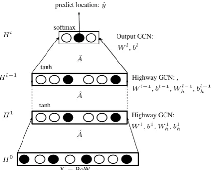
Highway GCN: Highway GCN: , Output GCN:
X=BoWtext
ˆ A ˆ A ˆ A
tanh
tanh softmax
H0 H1 Hl−1
Hl
predict location:yˆ
Wl−1,bl−1,Wl−1 h ,b
l−1 h
W1,b1,W1 h,b1h
[image:2.595.308.524.58.232.2]Wl,bl
Figure 1: The architecture of GCN geolocation model with layer-wise highway gates (Whi, bih).
GCN is applied to a BoW model of user content over the @-mention graph to predict user location.
where Wl andbl are learnable layer parameters, andnhood(i)indicates the neighbours of userui. Each extra layer in GCN extends the neighbour-hood over which a sample is smoothed. For ex-ample a GCN with 3 layers smooths each sex-ample with its neighbours up to 3 hops away, which is beneficial if location homophily extends to a neigh-bourhood of this size.
2.2.1 Highway GCN
Expanding the neighbourhood for label propaga-tion by adding multiple GCN layers can improve geolocation by accessing information from friends that are multiple hops away, but it might also lead to propagation of noisy information to users from an exponentially increasing number of expanded neighbourhood members. To control the required balance of how much neighbourhood information should be passed to a node, we use layer-wise gates similar to highway networks. In highway networks (Srivastava et al., 2015), the output of a layer is summed with its input with gating weightsT(~hl):
T(~hl) =σ
Wtl~hl+blt
~hl+1 =~hl+1◦T(~hl) +~hl◦(1−T(~hl)), (3)
where ~hl is the incoming input to layer l + 1, (Wl
t, blt) are gating weights and bias variables,◦is elementwise multiplication, andσis theSigmoid
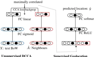
2.3 DCCA
Given two viewsX andAˆ(from Equation1) of data samples, CCA (Hotelling,1936), and its deep version (DCCA) (Andrew et al.,2013) learn func-tions f1(X) and f2( ˆA) such that the correlation between the output of the two functions is max-imised:
ρ= corr(f1(X), f2( ˆA)). (4)
The resulting representations off1(X)andf2( ˆA) are the compressed representations of the two views where the uncorrelated noise between them is reduced. The new representations ideally repre-sent user communities for the network view, and the language model of that community for the text view, and their concatenation is a multiview repre-sentation of data, which can be used as input for other tasks.
In DCCA, the two views are first projected to a lower dimensionality using a separate multilayer perceptron for each view (thef1andf2functions of Equation4), the output of which is used to estimate the CCA cost:
maximise: tr(W1TΣ12W2)
subject to: W1TΣ11W1=W2TΣ22W2 =I (5)
whereΣ11andΣ22are the covariances of the two outputs, and Σ12 is the cross-covariance. The weightsW1 andW2 are the linear projections of the MLP outputs, which are used in estimating the CCA cost. The optimisation problem is solved by SVD, and the error is backpropagated to train the parameters of the two MLPs and the final linear projections. After training, the two networks are used to predict new projections for unseen data. The two projections of unseen data — the outputs of the two networks — are then concatenated to form a multiview sample representation, as shown in Figure2.
3 Experiments
3.1 Data
We use three existing Twitter user geolocation datasets: (1) GEOTEXT(Eisenstein et al.,2010), (2) TWITTER-US (Roller et al., 2012), and (3) TWITTER-WORLD (Han et al., 2012). These datasets have been used widely for training and evaluation of geolocation models. They are all pre-partitioned into training, development and test
maximally correlated
FC sigmoid
FC softmax
X: text BoW Aˆ: Neighbours
predicted location:yˆ
FC linear
Unsupervised DCCA Supervised Geolocation
FC ReLU
[image:3.595.321.516.62.180.2]CCA loss backprop
Figure 2: TheDCCAmodel architecture: First the two text and network viewsXandAˆare fed into two neural networks (left), which are unsupervis-edly trained to maximise the correlation of their outputs; next the outputs of the networks are con-catenated, and fed as input to another neural net-work (right), which is trained supervisedly to pre-dict locations.
sets. Each user is represented by the concate-nation of their tweets, and labelled with the lat-itude/longitude of the first collected geotagged tweet in the case of GEOTEXTand TWITTER-US, and the centre of the closest city in the case of TWITTER-WORLD. GEOTEXTand TWITTER-US cover the continental US, and TWITTER-WORLD covers the whole world, with 9k, 449k and 1.3m users, respectively. The labels are the discretised geographical coordinates of the training points us-ing ak-d tree followingRoller et al.(2012), with the number of labels equal to 129, 256, and 930 for GEOTEXT, TWITTER-US, and TWITTER-WORLD, respectively.
3.2 Constructing the Views
We build matrixAˆas in Equation1using the col-lapsed @-mention graph between users, where two users are connected (Aij = 1) if one mentions the other, or they co-mention another user. The text view is a BoW model of user content with binary term frequency, inverse document frequency, and
l2normalisation of samples.
3.3 Model Selection
k-d tree bucket size hyperparameter which controls the maximum number of users in each cluster is set to 50, 2400, and 2400 for the respective datasets, based on tuning over the validation set. The archi-tecture ofGCN-LPis similar, with the difference that the text view is set to zero. InDCCA, for the unsupervised networks we use a single sigmoid hidden layer with size 1000 and a linear output layer with size 500 for the three datasets. The loss function is CCA loss, which maximises the output correlations. The supervised multilayer perceptron has one hidden layer with size 300, 600, 1000 for GEOTEXT, TWITTER-US, and TWITTER-WORLD, respectively, which we set by tuning over the devel-opment sets. We evaluate the models usingMedian error,Meanerror, andAcc@161, accuracy of pre-dicting a user within 161km or 100 miles from the known location.
3.4 Baselines
We also compareDCCA andGCN with two base-lines:
GCN-LP is based onGCN, but for input, instead of text-based features , we use one-hot encoding of a user’s neighbours, which are then convolved with theirk-hop neighbours using theGCN. This approach is similar to label propagation in smooth-ing the label distribution of a user with that of its neighbours, but uses graph convolutional networks which have extra layer parameters, and also a gat-ing mechanism to control the smoothgat-ing neighbour-hood radius. Note that for unlabelled samples, the predicted labels are used for input after training accuracy reaches 0.2.
MLP-TXT+NET is a simple transductive suvised model based on a single layer multilayer per-ceptron where the input to the network is the con-catenation of the text viewX, the user content’s bag-of-words andAˆ(Equation1), which represents the network view as a vector input. For the hidden layer we use a ReLU nonlinearity, and sizes 300, 600, and 600 for GEOTEXT, TWITTER-US, and TWITTER-WORLD, respectively.
4 Results and Analysis
4.1 Representation
Deep CCA and GCN are able to provide an un-supervised data representation in different ways.
Deep CCA takes the two text-based and network-based views, and finds deep non-linear transforma-tions that result in maximum correlation between the two views (Andrew et al.,2013). The represen-tations can be visualised using t-SNE, where we hope that samples with the same label are clustered together. GCN, on the other hand, uses graph con-volution. The representations of 50 samples from each of 4 randomly chosen labels of GEOTEXTare shown in Figure3. As shown, Deep CCA seems to slightly improve the representations from pure concatenation of the two views. GCN, on the other hand, substantially improves the representations. Further application of GCN results in more sam-ples clumping together, which might be desirable when there is strong homophily.
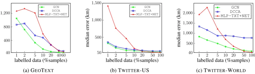
4.2 Labelled Data Size
To achieve good performance in supervised tasks, often large amounts of labelled data are required, which is a big challenge for Twitter geolocation, where only a small fraction of the data is geo-tagged (about 1%). The scarcity of supervision indicates the importance of semi-supervised learn-ing where unlabelled (e.g. non-geotagged) tweets are used for training. The three models we propose (MLP-TXT+NET, DCCA, and GCN) are all trans-ductive semi-supervised models that use unlabelled data, however, they are different in terms of how much labelled data they require to achieve accept-able performance. Given that in a real-world sce-nario, only a small fraction of data is geotagged, we conduct an experiment to analyse the effect of labelled samples on the performance of the three geolocation models. We provided the three mod-els with different fractions of samples that are la-belled (in terms of % of dataset samples) while using the remainder as unlabelled data, and anal-ysed theirMedianerror performance over the de-velopment set of GEOTEXT, TWITTER-US, and TWITTER-WORLD. Note that the text and net-work view, and the development set, remain fixed for all the experiments. As shown in Figure 4, when the fraction of labelled samples is less than 10% of all the samples, GCN and DCCA outper-formMLP-TXT+NET, as a result of having fewer parameters, and therefore, lower supervision re-quirement to optimise them. When enough training data is available (e.g. more than 20% of all the sam-ples),GCNandMLP-TXT+NETclearly outperform
(a)MLP-TXT+NET (b)DCCA (c) 1GCNAˆ·X (d) 2GCNAˆ·Aˆ·X
Figure 3: Comparing t-SNE visualisations of 50 training samples from each of 4 randomly chosen regions of GEOTEXTusing various data representations: (a) concatenation ofAˆ(Equation1); (b) concatenation ofDCCAtransformation of text-based and network-based viewsXandAˆ; (c) applying graph convolution
ˆ
A·X; and (d) applying graph convolution twiceAˆ·Aˆ·X
60 40 20 10 5 2 1 40 400 800 1,200
labelled data (%samples)
median
error
(km)
GCN DCCA MLP-TXT+NET
(a) GEOTEXT
100 50 20 10 5 2 1 50 500 1,000 1,500
labelled data (%samples)
median
error
(km)
GCN DCCA MLP-TXT+NET
(b) TWITTER-US
100 50 20 10 5 2 1 40 500 1,000 1,500 2,000
labelled data (%samples)
median
error
(km)
GCN DCCA MLP-TXT+NET
(c) TWITTER-WORLD
Figure 4: The effect of the amount of labelled data available as a fraction of all samples for GEO -TEXT, TWITTER-US, and TWITTER-WORLD on the development performance of GCN, DCCA, and
MLP-TXT+NETmodels in terms ofMedianerror. The dataset sizes are 9k, 440k, and 1.4m for the three datasets, respectively.
interactions between network and text views. When all the training samples of the two larger datasets (95% and 98% for TWITTER-US and TWITTER -WORLD, respectively) are available to the mod-els,MLP-TXT+NEToutperformsGCN. Note that the number of parameters increases fromDCCAto
GCNand toMLP-TXT+NET. In 1% for GEOTEXT,
DCCAoutperformsGCNas a result of having fewer parameters and just a few labelled samples, insuffi-cient to train the parameters ofGCN.
4.3 Highway Gates
Adding more layers to GCN expands the graph neighbourhood within which the user features are averaged, and so might introduce noise, and con-sequently decrease accuracy as shown in Figure5
when no gates are used. We see that by adding highway network gates, the performance ofGCN
slightly improves until three layers are added, but then by adding more layers the performance doesn’t change that much as gates are allowing the layer inputs to pass through the network without
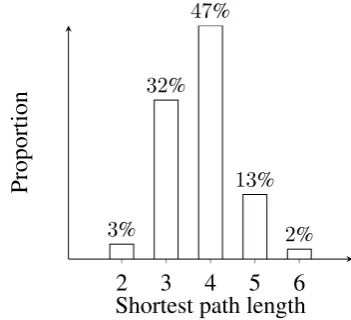
much change. The performance peaks at 4 layers which is compatible with the distribution of short-est path lengths shown in Figure6.
4.4 Performance
The performance of the three proposed models (MLP-TXT+NET,DCCAandGCN) is shown in Ta-ble1. The models are also compared with super-vised text-based methods (Wing and Baldridge,
2014; Cha et al., 2015; Rahimi et al.,2017b), a network-based method (Rahimi et al.,2015a) and
GCN-LP, and also joint text and network mod-els (Rahimi et al.,2017b;Do et al.,2017;Miura et al., 2017). MLP-TXT+NET and GCN outper-form all the text- or network-only models, and also the hybrid model of Rahimi et al. (2017b), indi-cating that joint modelling of text and network
features is important. MLP-TXT+NET is
[image:5.595.86.504.264.385.2]-GEOTEXT TWITTER-US TWITTER-WORLD
Acc@161↑ Mean↓ Median↓ Acc@161↑ Mean↓ Median↓ Acc@161↑ Mean↓ Median↓
Text (inductive)
Rahimi et al.(2017b) 38 844 389 54 554 120 34 1456 415
Wing and Baldridge(2014) — — — 48 686 191 31 1669 509
Cha et al.(2015) — 581 425 — — — — — —
Network (transductive)
Rahimi et al.(2015a) 58 586 60 54 705 116 45 2525 279
GCN-LP 58 576 56 53 653 126 45 2357 279
Text+Network (transductive)
Do et al.(2017) 62 532 32 66 433 45 53 1044 118
Miura et al.(2017) — — — 61 481 65 — — —
Rahimi et al.(2017b) 59 578 61 61 515 77 53 1280 104
MLP-TXT+NET 58 554 58 66 420 56 58 1030 53
DCCA 56 627 79 58 516 90 21 2095 913
GCN 60 546 45 62 485 71 54 1130 108
Text+Network (transductive)
MLP-TXT+NET1% 8 1521 1295 14 1436 1411 8 3865 2041
DCCA1% 7 1425 979 38 869 348 14 3014 1367
[image:6.595.75.526.65.278.2]GCN1% 6 1103 609 41 788 311 21 2071 853
Table 1: Geolocation results over the three Twitter datasets for the proposed models: joint text+network
MLP-TXT+NET,DCCA, andGCNand network-basedGCN-LP. The models are compared with text-only and network-only methods. The performance of the three joint models is also reported for minimal supervision scenario where only 1% of the total samples are labelled. “—” signifies that no results were reported for the given metric or dataset. Note thatDo et al.(2017) use timezone, andMiura et al.(2017) use the description and location fields in addition to text and network.
1 2 3 4 5 6 7 8 9 10 10
60 160 360 760
Number of layers
Median
(km)
[image:6.595.327.503.391.551.2]−highway +highway
Figure 5: The effect of adding more GCN layers (neighbourhood expansion) toGCNin terms of me-dian error over the development set of GEOTEXT with and without the highway gates, and averaged over5runs.
TEXT. However, it’s difficult to make a fair compar-ison as they use timezone data in their feature set.
MLP-TXT+NEToutperformsGCNover TWITTER -US and TWITTER-WORLD, which are very large, and have large amounts of labelled data. In a scenario with little supervision (1% of the total samples are labelled)DCCAandGCNclearly out-performMLP-TXT+NET, as they have fewer
pa-2 3 4 5 6
3%
32%
47%
13%
2%
Shortest path length
Proportion
Figure 6: The distribution of shortest path lengths between all the nodes of the largest connected com-ponent of GEOTEXT’s graph that constitute more than 1% of total.
rameters. Except forAcc@161over GEOTEXT where the number of labelled samples in the mini-mal supervision scenario is very low,GCN outper-formsDCCAby a large margin, indicating that for a medium dataset where only 1% of samples are labelled (as happens in random samples of Twit-ter)GCNis superior toMLP-TXT+NETandDCCA, consistent with Section4.2. BothMLP-TXT+NET
[image:6.595.81.284.391.549.2]to network-only, text-only, and hybrid models. The network-basedGCN-LPmodel, which does label propagation using Graph Convolutional Networks, outperformsRahimi et al.(2015a), which is based on location propagation using Modified Adsorp-tion (Talukdar and Crammer,2009), possibly be-cause the label propagation inGCNis parametrised.
4.5 Error Analysis
Although the performance of MLP-TXT+NETis
better thanGCN andDCCAwhen a large amount of labelled data is available (Table1), under a sce-nario where little labelled data is available (1% of data),DCCAandGCNoutperformMLP-TXT+NET, mainly because the number of parameters in
MLP-TXT+NET grows with the number of sam-ples, and is much larger thanGCNandDCCA.GCN
outperformsDCCAandMLP-TXT+NETusing 1%
of data, however, the distribution of errors in the development set of TWITTER-US indicates higher error for smaller states such as Rhode Island (RI), Iowa (IA), North Dakota (ND), and Idaho (ID), which is simply because the number of labelled samples in those states is insufficient.
Although we evaluate geolocation models with
Median,Mean, andAcc@161, it doesn’t mean
that the distribution of errors is uniform over all locations. Big cities often attract more local online discussions, making the geolocation of users in those areas simpler. For example users in LA are more likely to talk about LA-related issues such as their sport teams, Hollywood or local events than users in the state of Rhode Island (RI), which lacks large sport teams or major events. It is also possible that people in less densely populated areas are further apart from each other, and therefore, as a result of discretisation fall in different clusters. The non-uniformity in local discussions results in lower geolocation performance in less densely populated areas like Midwest U.S., and higher performance in densely populated areas such as NYC and LA as shown in Figure7. The geographical distribution of error forGCN,DCCAandMLP-TXT+NETunder the minimal supervision scenario is shown in the supplementary material.
To get a better picture of misclassification be-tween states, we built a confusion matrix based on known state and predicted state for development users of TWITTER-US usingGCNusing only 1% of labelled data. There is a tendency for users to be wrongly predicted to be in CA, NY, TX, and
surpris-ingly OH. Particularly users from states such as TX, AZ, CO, and NV, which are located close to CA, are wrongly predicted to be in CA, and users from NJ, PA, and MA are misclassified as being in NY. The same goes for OH and TX where users from neighbouring smaller states are misclassified to be there. Users from CA and NY are also misclas-sified between the two states, which might be the result of business and entertainment connections that exist between NYC and LA/SF. Interestingly, there are a number of misclassifications to FL for users from CA, NY, and TX, which might be the effect of users vacationing or retiring to FL. The full confusion matrix between the U.S. states is provided in the supplementary material.
4.6 Local Terms
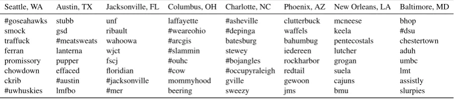
In Table2, local terms of a few regions detected byGCNunder minimal supervision are shown. The terms that were present in the labelled data are excluded to show how graph convolutions over the social graph have extended the vocabulary. For example, in case of Seattle, #goseahawks is an important term not present in the 1% labelled data but present in the unlabelled data. The convolution over the social graph is able to utilise such terms that don’t exist in the labelled data.
5 Related Work
Previous work on user geolocation can be broadly divided into text-based, network-based and multi-view approaches.
Text-based geolocation uses the geographical bias in language use to infer the location of users. There are three main text-based approaches to ge-olocation: (1) gazetteer-based models which map geographical references in text to location, but ig-nore non-geographical references and vernacular uses of language (Rauch et al.,2003;Amitay et al.,
2004; Lieberman et al., 2010); (2) geographical topic models that learn region-specific topics, but don’t scale to the magnitude of social media ( Eisen-stein et al.,2010;Hong et al.,2012;Ahmed et al.,
2013); and (3) supervised models which are of-ten framed as text classification (Serdyukov et al.,
2009; Wing and Baldridge, 2011; Roller et al.,
2012;Han et al.,2014) or text regression (Iso et al.,
MN
WA MT
ID
ND
ME WI
OR SD MI VTNH
NY WY
IA
NE MA
IL
PA CT RI
CA NV
UT CO IN OH WV NJ
MO
KS DE
MD VA KY
DC
AZ
OK
NM TN NC
TX
AR
SC AL
GA MS
LA
FL
100 200 300 400 500 600 700 800
median
error
[image:8.595.80.525.71.236.2](km)
Figure 7: The geographical distribution ofMedianerror ofGCNusing 1% of labelled data in each state over the development set of TWITTER-US. The colour indicates error and the size indicates the number of development users within the state.
Seattle, WA Austin, TX Jacksonville, FL Columbus, OH Charlotte, NC Phoenix, AZ New Orleans, LA Baltimore, MD
#goseahawks stubb unf laffayette #asheville clutterbuck mcneese bhop
smock gsd ribault #weareohio #depinga waffels keela #dsu
traffuck #meatsweats wahoowa #arcgis batesburg bahumbug pentecostals chestertown
ferran lanterna wjct #slammin stewey iedereen lutcher aduh
promissory pupper fscj #ouhc #bojangles rockharbor grogan umbc
chowdown effaced floridian #cow #occupyraleigh redtail suela lmt
ckrib #austin #jacksonville mommyhood gville gewoon cajuns assistly
#uwhuskies lmfbo #mer beering sweezy jms bmu slurpies
Table 2: Top terms for selected regions detected byGCNusing only 1% of TWITTER-US for supervision. We present the terms that were present only in unlabelled data. The terms include city names, hashtags, food names and internet abbreviations.
Network-based methods leverage the location homophily assumption: nearby users are more likely to befriend and interact with each other. There are four main network-based geolocation ap-proaches: distance-based, supervised classification, graph-based label propagation, and node embed-ding methods. Distance-based methods model the probability of friendship given the distance ( Back-strom et al.,2010;McGee et al.,2013;Gu et al.,
2012;Kong et al.,2014), supervised models use neighbourhood features to classify a user into a location (Rout et al., 2013; Malmi et al., 2015), and graph-based label-propagation models propa-gate the location information through the user–user graph to estimate unknown labels (Davis Jr et al.,
2011;Jurgens,2013;Compton et al.,2014). Node embedding methods build heterogeneous graphs between user–user, user–location and location– location, and learn an embedding space to minimise the distance of connected nodes, and maximise the distance of disconnected nodes. The embeddings
are then used in supervised models for geoloca-tion (Wang et al.,2017). Network-based models fail to geolocate disconnected users:Jurgens et al.
(2015) couldn’t geolocation 37% of users as a re-sult of disconnectedness.
Previous work on hybrid text and network meth-ods can be broadly categorised into three main ap-proaches: (1) incorporating text-based information such as toponyms or locations predicted from a text-based model as auxiliary nodes into the user–user graph, which is then used in network-based mod-els (Li et al.,2012a,b;Rahimi et al.,2015b,a); (2) ensembling separately trained text- and network-based models (Gu et al., 2012;Ren et al., 2012;
[image:8.595.72.524.308.407.2]multiview approaches — with the exception ofLi et al.(2012a) andLi et al. (2012b) that only use toponyms — effectively uses unlabelled data in the text view, and use only the unlabelled information of the network view via the user–user graph.
There are three main shortcomings in the previ-ous work on user geolocation that we address in this paper: (1) with the exception of few recent works (Miura et al., 2017; Do et al., 2017), pre-vious models don’t jointly exploit both text and network information, and therefore the interaction between text and network views is not modelled; (2) the unlabelled data in both text and network views is not effectively exploited, which is crucial given the small amounts of available supervision; and (3) previous models are rarely evaluated under a minimal supervision scenario, a scenario which reflects real world conditions.
6 Conclusion
We proposed GCN, DCCA and MLP-TXT+NET,
three multiview, transductive, semi-supervised ge-olocation models, which use text and network in-formation to infer user location in a joint setting. We showed that joint modelling of text and network information outperforms network-only, text-only, and hybrid geolocation models as a result of mod-elling the interaction between text and network information. We also showed thatGCNandDCCA
are able to perform well under a minimal super-vision scenario similar to real world applications by effectively using unlabelled data. We ignored the context in which users interact with each other, and assumed all the connections to hold location homophily. In future work, we are interested in modelling the extent to which a social interaction is caused by geographical proximity (e.g. using user–user gates).
References
Amr Ahmed, Liangjie Hong, and Alexander J. Smola. 2013. Hierarchical geographical modeling of user locations from social media posts. InProceedings of the 22nd International Conference on World Wide Web (WWW 2013), pages 25–36, Rio de Janeiro, Brazil.
Einat Amitay, Nadav Har’El, Ron Sivan, and Aya Sof-fer. 2004. Web-a-where: geotagging web content. In Proceedings of the 27th Annual International ACM SIGIR Conference on Research and Develop-ment in Information Retrieval (SIGIR 2004), pages 273–280, Sheffield, UK.
Galen Andrew, Raman Arora, Jeff Bilmes, and Karen Livescu. 2013. Deep canonical correlation analysis. In International Conference on Machine Learning, pages 1247–1255, Atlanta, USA.
Lars Backstrom, Eric Sun, and Cameron Marlow. 2010. Find me if you can: improving geographical predic-tion with social and spatial proximity. In Proceed-ings of the 19th International Conference on World Wide Web (WWW 2010), pages 61–70, Raleigh, USA.
Miriam Cha, Youngjune Gwon, and H.T. Kung. 2015. Twitter geolocation and regional classification via sparse coding. In Proceedings of the 9th Inter-national Conference on Weblogs and Social Media (ICWSM 2015), pages 582–585, Oxford, UK.
Zhiyuan Cheng, James Caverlee, and Kyumin Lee. 2010. You are where you tweet: a content-based ap-proach to geo-locating Twitter users. InProceedings of the 19th ACM International Conference Infor-mation and Knowledge Management (CIKM 2010), pages 759–768, Toronto, Canada.
Jaime Chon, Ross Raymond, Haiyan Wang, and Feng Wang. 2015. Modeling flu trends with real-time geo-tagged twitter data streams. InProceedings of the 10th International Conference on Wireless Al-gorithms, Systems, and Applications (WASA 2015), pages 60–69, Qufu, China.
Ryan Compton, David Jurgens, and David Allen. 2014. Geotagging one hundred million twitter accounts with total variation minimization. InProceedings of the IEEE International Conference on Big Data (IEEE BigData 2014), pages 393–401, Washington DC, USA.
Clodoveu A Davis Jr, Gisele L Pappa, Diogo
Renn´o Rocha de Oliveira, and Filipe de L Arcanjo. 2011. Inferring the location of twitter messages based on user relationships. Transactions in GIS, 15(6):735–751.
Bertrand De Longueville, Robin S. Smith, and Gian-luca Luraschi. 2009. ”omg, from here, i can see the flames!”: A use case of mining location based social networks to acquire spatio-temporal data on forest fires. InProceedings of the 2009 International Work-shop on Location Based Social Networks, pages 73– 80, New York, USA.
Tien Huu Do, Duc Minh Nguyen, Evaggelia Tsili-gianni, Bruno Cornelis, and Nikos Deligiannis. 2017. Multiview deep learning for predicting twitter users’ location. arXiv preprint arXiv:1712.08091.
Hansu Gu, Haojie Hang, Qin Lv, and Dirk Grun-wald. 2012. Fusing text and frienships for location inference in online social networks. In Proceed-ings of the The 2012 IEEE/WIC/ACM International Joint Conferences on Web Intelligence and Intelli-gent AIntelli-gent Technology - Volume 01, volume 1, pages 158–165, Macau, China.
Bo Han, Paul Cook, and Timothy Baldwin. 2012. Ge-olocation prediction in social media data by find-ing location indicative words. In Proceedings of the 24th International Conference on Compu-tational Linguistics (COLING 2012), pages 1045– 1062, Mumbai, India.
Bo Han, Paul Cook, and Timothy Baldwin. 2014. Text-based Twitter user geolocation prediction. Journal of Artificial Intelligence Research, 49:451–500.
Brent Hecht, Lichan Hong, Bongwon Suh, and Ed H. Chi. 2011. Tweets from Justin Bieber’s heart: the dynamics of the location field in user profiles. In
Proceedings of the SIGCHI Conference on Human Factors in Computing Systems, pages 237–246, Van-couver, Canada.
Liangjie Hong, Amr Ahmed, Siva Gurumurthy, Alexan-der J. Smola, and Kostas Tsioutsiouliklis. 2012. Dis-covering geographical topics in the twitter stream. InProceedings of the 21st international conference on World Wide Web, pages 769–778, Lyon, France.
Harold Hotelling. 1936. Relations between two sets of variates.Biometrika, 28(3/4):321–377.
Hayate Iso, Shoko Wakamiya, and Eiji Aramaki. 2017. Density estimation for geolocation via convolu-tional mixture density network. arXiv preprint arXiv:1705.02750.
Gaya Jayasinghe, Brian Jin, James Mchugh, Bella Robinson, and Stephen Wan. 2016. CSIRO Data61 at the WNUT geo shared task. InProceedings of the COLING 2016 Workshop on Noisy User-generated Text (W-NUT 2016), pages 218–226, Osaka, Japan.
David Jurgens. 2013. That’s what friends are for: Infer-ring location in online social media platforms based on social relationships. InProceedings of the 7th In-ternational Conference on Weblogs and Social Me-dia (ICWSM 2013), pages 273–282, Boston, USA.
David Jurgens, Tyler Finethy, James McCorriston, Yi Tian Xu, and Derek Ruths. 2015. Geolocation prediction in twitter using social networks: A critical analysis and review of current practice. In Proceed-ings of the 9th International Conference on Weblogs and Social Media (ICWSM 2015), pages 188–197, Oxford, UK.
Thomas N. Kipf and Max Welling. 2017. Semi-supervised classification with graph convolutional networks. InInternational Conference on Learning Representations (ICLR).
Longbo Kong, Zhi Liu, and Yan Huang. 2014. Spot: Locating social media users based on social net-work context.Proceedings of the VLDB Endowment, 7(13):1681–1684.
Rui Li, Shengjie Wang, and Kevin Chen-Chuan Chang. 2012a. Multiple location profiling for users and rela-tionships from social network and content. Proceed-ings of the VLDB Endowment, 5(11):1603–1614.
Rui Li, Shengjie Wang, Hongbo Deng, Rui Wang, and Kevin Chen-Chuan Chang. 2012b. Towards social user profiling: unified and discriminative influence model for inferring home locations. In Proceed-ings of the 18th ACM SIGKDD International Con-ference on Knowledge Discovery and Data Mining (SIGKDD 2012), pages 1023–1031, Beijing, China.
Michael D Lieberman, Hanan Samet, and Jagan Sankaranarayanan. 2010. Geotagging with local lex-icons to build indexes for textually-specified spatial data. InProceedings of the 26th International Con-ference on Data Engineering (ICDE 2010), pages 201–212, Long Beach, USA.
Eric Malmi, Arno Solin, and Aristides Gionis. 2015. The blind leading the blind: Network-based loca-tion estimaloca-tion under uncertainty. In Proceedings of the European Conference on Machine Learning and Principles and Practice of Knowledge Discov-ery in Databases 2015 (ECML PKDD 2015), pages 406–421, Porto, Portugal.
Jeffrey McGee, James Caverlee, and Zhiyuan Cheng. 2013. Location prediction in social media based on tie strength. In Proceedings of the 22nd ACM international conference on Conference on informa-tion & knowledge management, pages 459–468, San Fransisco, USA. ACM.
Yasuhide Miura, Motoki Taniguchi, Tomoki Taniguchi, and Tomoko Ohkuma. 2017. Unifying text, meta-data, and user network representations with a neural network for geolocation prediction. InProceedings of the 55th Annual Meeting of the Association for Computational Linguistics (Volume 1: Long Papers), volume 1, pages 1260–1272, Vancouver, Canada.
Fred Morstatter, J¨urgen Pfeffer, Huan Liu, and Kath-leen M Carley. 2013. Is the sample good enough? Comparing data from Twitter’s streaming API with Twitter’s firehose. InProceedings of the 7th Inter-national Conference on Weblogs and Social Media (ICWSM 2013), pages 400–408, Boston, USA.
Michael J. Paul and Mark Dredze. 2011. You are what you tweet: Analyzing twitter for public health. In
Proceedings of the Fifth International Conference on Weblogs and Social Media (ICSWM 2011), pages 265–272, Barcelona, Spain.
Processing (EMNLP 2017), pages 167–176, Copen-hagen, Denmark.
Afshin Rahimi, Trevor Cohn, and Timothy Baldwin. 2015a. Twitter user geolocation using a unified text and network prediction model. InProceedings of the 53rd Annual Meeting of the Association for Computational Linguistics — 7th International Joint Conference on Natural Language Processing (ACL-IJCNLP 2015), pages 630–636, Beijing, China.
Afshin Rahimi, Trevor Cohn, and Timothy Baldwin. 2017b. A neural model for user geolocation and lexical dialectology. InProceedings of the 55th An-nual Meeting of the Association for Computational Linguistics (ACL 2017), pages 207–216, Vancouver, Canada.
Afshin Rahimi, Duy Vu, Trevor Cohn, and Timo-thy Baldwin. 2015b. Exploiting text and network context for geolocation of social media users. In
Proceedings of the 2015 Conference of the North American Chapter of the Association for Compu-tational Linguistics — Human Language Technolo-gies (NAACL HLT 2015), pages 1362–1367, Denver, USA.
Erik Rauch, Michael Bukatin, and Kenneth Baker. 2003. A confidence-based framework for disam-biguating geographic terms. InProceedings of the HLT-NAACL 2003 workshop on Analysis of geo-graphic references-Volume 1, pages 50–54, Edmon-ton, Canada.
Kejiang Ren, Shaowu Zhang, and Hongfei Lin. 2012. Where are you settling down: Geo-locating Twitter users based on tweets and social networks. In Pro-ceedings of the 8th Asia Information Retrieval Soci-eties Conference (AIRS 2012), pages 150–161, Tian-jin, China.
Silvio Ribeiro and Gisele L. Pappa. 2017. Strategies for combining Twitter users geo-location methods.
GeoInformatica, pages 1–25.
Stephen Roller, Michael Speriosu, Sarat Rallapalli, Benjamin Wing, and Jason Baldridge. 2012. Super-vised text-based geolocation using language models on an adaptive grid. In Proceedings of the 2012 Joint Conference on Empirical Methods in Natural Language Processing and Computational Natural Language Learning (EMNLP-CONLL 2012), pages 1500–1510, Jeju, South Korea.
Dominic Rout, Kalina Bontcheva, Daniel Preot¸iuc-Pietro, and Trevor Cohn. 2013. Where’s @wally?: A classification approach to geolocating users based on their social ties. InProceedings of the 24th ACM Conference on Hypertext and Social Media (Hyper-text 2013), pages 11–20, Paris, France.
Takeshi Sakaki, Makoto Okazaki, and Yutaka Matsuo. 2010. Earthquake shakes twitter users: Real-time event detection by social sensors. In Proceedings of the 19th International Conference on World Wide Web, pages 851–860, New York, USA.
Pavel Serdyukov, Vanessa Murdock, and Roelof Van Zwol. 2009. Placing Flickr photos on a map. In
Proceedings of the 32nd International ACM SIGIR Conference on Research and Development in Infor-mation Retrieval, pages 484–491, Boston, USA.
Rupesh Kumar Srivastava, Klaus Greff, and J¨urgen Schmidhuber. 2015. Highway networks. arXiv preprint arXiv:1505.00387.
Partha Pratim Talukdar and Koby Crammer. 2009. New regularized algorithms for transductive learn-ing. In Proceedings of the European Conference on Machine Learning (ECML-PKDD 2009), pages 442–457, Bled, Slovenia.
Fengjiao Wang, Chun-Ta Lu, Yongzhi Qu, and S Yu Philip. 2017. Collective geographical embedding for geolocating social network users. In Proceed-ings of the Pacific-Asia Conference on Knowledge Discovery and Data Mining (PAKDD 2017), pages 599–611, Jeju, South Korea.
Benjamin P Wing and Jason Baldridge. 2011. Sim-ple supervised document geolocation with geodesic grids. InProceedings of the 49th Annual Meeting of the Association for Computational Linguistics: Hu-man Language Technologies-Volume 1 (ACL-HLT 2011), pages 955–964, Portland, USA.
Benjamin P Wing and Jason Baldridge. 2014. Hierar-chical discriminative classification for text-based ge-olocation. In Proceedings of the 2014 Conference on Empirical Methods in Natural Language Process-ing (EMNLP 2014), pages 336–348, Doha, Qatar.