The Effects of Process R&D in an Asymmetric Duopoly under Cournot and Supply Function Competitions

Munich Personal RePEc Archive

The Effects of Process RD in an

Asymmetric Duopoly under Cournot and

Supply Function Competitions

Saglam, Ismail

Ankara, Turkey

26 April 2018

Online at

https://mpra.ub.uni-muenchen.de/86385/

The Effects of Process R&D in an Asymmetric Duopoly under

Cournot and Supply Function Competitions

Ismail Saglam

Ankara, Turkey

Abstract. In this paper we attempt to explore the welfare effects of (process) R&D in an asymmetric duopoly with a homogeneous product under Cournot and supply function competitions. To this aim, we consider a two-stage perfect-information game where the duopolists compete in stage one in R&D investments and in stage two either in quantities or in supply functions. Calculating the (subgame-perfect Nash) equilibrium of this game numerically for a wide range of initial cost parameters and comparing it to the equilibrium with no R&D, we show that R&D has a positive effect on the welfares of consumers and the society as a whole. While its effect on the profits of the duopolists is also positive under the Cournot competition, it becomes negative under the supply function competition. This latter negative effect is caused by the duopolists’ more aggressively investing in R&D under the supply function competition, increasing the industry output, and consequently decreasing the product price, to a harmful level for themselves. Moreover, we show that R&D always widens up the efficiency gap between the duopolists under the supply function competition, while narrowing it down under the Cournot competition.

Keywords: Duopoly; Cournot competition; supply function competition; process R&D

JEL Codes: D43; L13

1

Introduction

or product R&D prior to production. A somewhat surprising answer to this question was obtained by Qiu (1997), showing that in a differentiated duopoly with process R&D, the Cournot competition in the output market always induces a higher R&D effort than the Bertrand competition, while the outcome of the Cournot competition can become more efficient than the outcome of the Bertrand competition if the duopolistic products are close substitutes and R&D productivity as well as spillovers in the output of R&D are sufficiently high. In fact, the same results were later shown to also hold when the R&D competition model of Qiu (1997) is modified to involve product R&D (as in Symeonidis, 2013) instead of process R&D or modified to involve input spillovers in R&D (as in Hinloopen and Vandekerckhove, 2009) instead of output spillovers.

In our model, we consider process R&D as in Qiu (1997) and Hinloopen and Vandekerckhove (2009). However, unlike these two works, we allow for neither spillovers in R&D nor differentiation in the output market. Moreover, we consider the supply function competition in the output market in comparison to the Cournot competition. To give more details, we model the R&D and production process as a two-stage perfect-information game where the duopolists non-cooperatively choose in the first stage their R&D investments and in the second stage either their supply functions or their quantities. Calculating the subgame-perfect Nash equilibrium (Selten, 1965) of this game numerically for a wide range of initial cost parameters and comparing it to the equilibrium with no R&D, we show that R&D has always a positive effect on the welfares of consumers and the society as a whole. While its effect on the profits of the duopolists is also positive under the Cournot competition, it becomes negative under the supply function competition. This latter negative effect is caused by the duopolists’ more aggressively investing in R&D under the supply function competition, increasing the industry output, and consequently decreasing the product price, to a harmful level for themselves. Moreover, we show that R&D always widens up the efficiency gap between the duopolists under the supply function competition, while narrowing it down under the Cournot competition.

R&D.

The rest of the paper is organized as follows: In Section 2, we present our model. Section 3 contains our results and Section 4 concludes.

2

Model

We consider a duopolistic industry where a single homogeneous good is produced under cost asymmetry. Firm i= 1,2 faces the cost function

Ci(qi) =ci(xi)q2

i/2, (1)

where qi is the quantity produced by firmiand ci(xi)>0 is its unitary marginal cost that is affected by the variablexi≥0, denoting the investment in process R&D (hereafter, simply R&D) by firmi. We assume that the common R&D technology of the firms is such that for each i= 1,2

ci(xi) =ci,0exp(−xi), (2) wherexi ≥0 andc1,0< c2,0, i.e., before any R&D takes place in the industry, firm 1 has a lower unitary marginal cost than firm 2. (Therefore, in many places firms 1 and 2 will be simply called the efficient and inefficient firms, respectively.) Also note that the technology in (2) implies no R&D spillovers, i.e., for any i, j∈ {1,2}withj=6 i,∂ci(xi)/∂xj = 0.

Investing in R&D is costly for each firm. Any firm investing inx≥0 units of R&D incurs a quadratic cost (as in d’Aspremont and Jacquemin, 1988):

z(x) =δx2

/2, (3)

where δ is a parameter that is positive. Note that according to (3), the marginal cost of R&D is increasing and independent of the size of the firm. Finally, we assume that the demand curve faced by the duopolistic firms is given by

D(p) =a−bp, (4)

where a, b > 0 are the intercept and slope parameters and p ∈ [0, a/b] denotes the product price. Equations (1)-(4) as well as the parametersc1,0, c2,0,δ, a, and bare common knowledge.

3

Results

3.1

Supply Function Competition with R&D Investment

Here, we will consider the case where the duopolistic firms compete in supply functions in the second stage game.1

Formally, a stage-two strategy for firm i = 1,2 is a linear function mapping prices into quantities, i.e.,Si =ηipwhereηi≥0. Given the strategiesS1 and S2, the duopolistic product market clears if

D(p) =S1(p) +S2(p) (5) or

a−bp=η1p+η2p, (6) implying an equilibrium pricepSF _(η

1, η2)≡pSF(η2, η1), given by

pSF _(η 1, η2) =

a b+η1+η2

. (7)

A pair of supply functions (S∗

1(p), S2∗(p)) = (η1∗p, η2∗p) forms a Nash (1950) equilibrium if for each

i, j ∈ {1,2} with j 6= i the function S∗

i(p) maximizes the expected profits of firm i when firm j produces according to the function S∗

j(p). That is, (η1∗p, η2∗p) forms a Nash (1950) equilibrium if for eachi, j∈ {1,2} withj6=ithe parameterη∗

i solves

max ηi≥0p

SF _η i, η∗j

S∗

i (p(ηi, ηj∗)

−ci(xi)

2 S

∗

i(p(ηi, ηj∗)) 2

−z(xi), (8)

or explicitly

max ηi≥0

ηi−

ci(xi)η2 i 2

a b+ηi+η∗j

!2

−z(xi). (9)

Proposition 1. Given the R&D levelsx1 and x2 determined in the first stage of the duopolistic game,

the stage-two competition in linear supply functions has a unique Nash equilibrium characterized by

SSF

i (p) =ηSFi (xi, xj)pfor eachi, j∈ {1,2} with j6=i, where

ηiSF(xi, xj) =

2

ci(xi) +

s

ci(xi)2+ 4

b

_{ci(xi) +cj(xj) +bci(xi)c}

j(xj) 2 +bcj(xj)

. (10)

Proof. If the pair of supply functions hηSF

1 (x1, x2)p, η2SF(x2, x1)pi forms a Nash (1950) equilibrium, then for eachi, j∈ {1,2} withj6=ithe pricepSF _ηSF

1 (x1, x2), η2SF(x2, x1)

must solve

max

p≥0 p a−bp−S SF j (p)

−ci(xi)

2 a−bp−S SF j (p)

2

−z(xi). (11)

1_{The supply function competition model we consider here is an adaptation of the symmetric oligopoly model of}

The first-order necessary condition for the above maximization implies

0 = a−bp−SjSF(p)

+ p−ci(xi) a−bp−SjSF(p)

−b−∂S

SF j (p)

∂p

!

, (12)

or

0 = SSF

i (p) + p−ci(xi)SiSF(p)

−b−ηSF j (xj, xi)

= ηSF

i (xi, xj)p+ p−ci(xi)ηSFi (xi, xj)p

−b−ηSF j (xj, xi)

, (13)

implying

ηSF

i (xi, xj) =

b+ηSF j (xj, xi) 1 +ci(xi)(b+ηSF

j (xj, xi))

. (14)

LetηSF

i ≡ηiSF(xi, xj) andηSFj ≡ηSFj (xj, xi). Then, equation (14) implies 1

ηSF i

= 1

b+ηSF j

+ci(xi) (15)

and 1

ηSF j

= 1

b+ηSF i

+cj(xj). (16)

Define Ei= 1/ηiSF andEj = 1/(b+ηSFj ). Then, (15) and (16) imply

Ei=Ej+ci(xi) (17) and

1 1

Ej

−b

= ₁1

Ei +b

+cj(xj). (18)

Inserting (17) into (18) and with the help of some arrangements we obtain

Ej 1−bEj

= (1 +bcj(xj))Ej+ci(xi) +cj(xi) +bci(xi)cj(xj) 1 +bEj+bci(xi)

. (19)

It follows from (19) that

E2

j +ci(xi)Ej−

ci(xi) +cj(xj) +bci(xi)cj(xj)

b(2 +bcj(xj)) = 0. (20) The positive-valued solution to the above quadratic equation can be calculated as

Ej=

−ci(xi) +

s

ci(xi)2₊4

b

_c

i(xi) +cj(xj) +bci(xi)cj(xj) 2 +bcj(xj)

Then using (17) and Ei = 1/ηiSF, we obtain (10). To check the second-order sufficiency condition, we differentiate the right-hand side of (12) with respect to pto obtain (−b−ηSF

j (xj, xi)) + (1 +ci(xi)(b+

ηSF

j (xj, xi)))(−b−ηjSF(xj, xi))<0 for all p≥0. So,pSF(η1SF(x1, x2), η2SF(x2, x1)) solves the problem in (11), implying that the supply functions ηSF

1 (x1, x2)pandηSF2 (x2, x1)pform a Nash equilibrium in

the second-stage game.

Define pSF_(x

1, x2) ≡pSF η1SF(x1, x2), ηSF2 (x2, x1)

for any x1 and x2. Note that q1SF(x1, x2) =

ηSF

1 (x1, x2)pSF(x1, x2) and q2SF(x2, x1) =η2SF(x2, x1)pSF(x1, x2). Perfectly anticipating the equilib-rium supply functions that would be chosen in the second stage of the duopolistic game, firm i can calculate in the first stage its profitsπSF

i (xi, xj), at each possible investment pair (xi, xj) wherej 6=i, as follows:

πiSF(xi, xj) = pSF(xi, xj)qSFi (xi, xj)−

ci(xi) 2 q

SF

i (xi, xj) 2

−z(xi) (22)

We say that a pair of R&D investment strategies (xSF

1 , xSF2 ) forms a Nash equilibrium of the reduced game in stage one if for eachi, j∈ {1,2}withj6=i,xSF

i maximizes the expected profits of firmiwhen firmj investsxSF

j . That is, for eachi, j∈ {1,2} withj6=i, the R&D levelxSFi solves max

xi≥0

πSF

i (xi, xSFj ). (23)

Given an equilibrium (xSF

1 , xSF2 ), involving the solution to (23) for each firm, it follows that the strategy profileh(xSF

1 , xSF2 ),(ηSF1 (xSF1 , xSF2 ), η2SF(xSF2 , xSF1 ))iconstitutes a subgame-perfect Nash equilibrium of the two-stage game played by the duopolists. At this equilibrium, the profits obtained by firmibecome

πiSF(xSFi , xSFj ) = ηSFi xSFi , xSFj

pSF xSFi , xSFj

2

−ci x

SF i

2 η SF

i xSFi , xSFj

2

pSF xSFi , xSFj

2 −δ 2 x SF i 2 . (24) LetQSF_(x

1, x2)≡q1SF(x1, x2) +q2SF(x2, x1). Then the equilibrium consumer surplus becomes

CSSF(xSF1 , x SF 2 ) =

QSF _xSF 1 , xSF2

2

2b

=

ηSF

1 (xSF1 , xSF2 ) +η2SF(xSF2 , xSF1 )

2

pSF_(xSF 1 , xSF2 )

2

2b . (25)

We leave the calculation ofxSF

i andxSFj as well as the corresponding equilibrium outputs and welfares to Section 3.3.

3.2

Cournot Competition with R&D Investment

i andj, the product market clears at a pricepC_(q i, qj) if

D(pC_(q

i, qj)) =qi+qj, (26)

implying

pC(qi, qj) =

a−qi−qj

b . (27)

A pair of quantities (q∗

1, q∗2) forms a (Cournot) Nash equilibrium in the second stage game if for each

i, j∈ {1,2}withj 6=ithe quantityq∗

i maximizes the expected profits of firmiwhen firmjproduces the quantity q∗

j. That is, (q1∗, q2) forms a Nash equilibrium if for each∗ i, j ∈ {1,2} withj 6=ithe quantity

q∗

i solves

max qi≥0 p

C_(q

i, q∗j)qi−

ci(xi) 2 q

2

i −z(xi). (28)

Proposition 2.Given the R&D levelsx1andx2determined in the first stage of the duopolistic game, the

stage-two competition in quantities has a unique Nash equilibrium characterized byhqC

1(x1, x2), qC2(x2, x1)i

such that for eachi, j∈ {1,2}with j6=i,

qiC(xi, xj) =

1 +bcj(xj)

(2 +bci(xi))(2 +bcj(xj))−1. (29)

Proof. The first-order necessary condition associated with the maximization problem in (28) is given by

−1

bqi+

a−qi−q∗j

b −ci(xi)qi= 0. (30)

If (q∗

1, q2∗) = (q1C, q2C) forms a Nash equilibrium, then for each i, j ∈ {1,2} with j 6= i the quantity

qi=qCi must satisfy the above first-order condition when q

∗

j =qjC, implying

qC i =

a−qC j

2 +bci(xi). (31)

Changing the role of iandj in (31), we can also get

qC j =

a−qC i 2 +bcj(xj)

. (32)

Then, solving (31) and (32) together, we can obtainqC

i (x1, x2) as in (29). To check the second-order suffi-ciency condition, we differentiate the left-hand side of (30) with respect toqito obtain−(2/b)−ci(xi)<0 for all qi ≥ 0. So, the quantity qiC(xi, xj) solves the problem in (28), implying that the strategies

qC

1(x1, x2) andq2C(x2, x1) form a Nash equilibrium in the second-stage game. .

Define pC_(x

i, xj) ≡ pC(qCi (xi, xj), qjC(xj, xi)) using (27) and (29) and also define QC(x1, x2) ≡

qC

second stage of the duopolistic game, firmican calculate in the first stage its profitsπC

i (xi, xj), at each possible investment pair (xi, xj) wherej6=i, as follows:

πC

i (xi, xj) = pC(xi, xj)qiC(xi, xj)−

ci(xi) 2 q

C i (xi, xj)

2

−z(xi) (33)

A pair of R&D investment strategies (xC

1, xC2) forms a Nash equilibrium if for each i, j ∈ {1,2} with

j 6=i, xC

i maximizes the expected profits of firm i when the R&D level of firm j is xCj. That is, xCi solves

max xi≥0 π

C

i (xi, xCj). (34)

Given an equilibrium (xC

1, xC2), involving the solution to (34) for each firm, it follows that the strategy profileh(xC

1, xC2),(q1C(xC1, xC2), q2C(xC2, xC1))iconstitutes a subgame-perfect Nash equilibrium of the two-stage game played by the duopolists. At this equilibrium, the profits of firmibecome

πC

i (xCi , xCj ) =pC(xCi , xCj)qCi (xCi , xCj)−

ci(xC i ) 2 q

C

i (xCi , xCj) 2

−δ

2(x C i )

2

, (35)

whereas the consumer surplus becomes

CSC(xC1, xC2) =

QC_(xC 1, xC2)

2

2b . (36)

3.3

The Output and Welfare Effects of R&D Investment

Due to the functional complexity of the optimization programs in (23) and (34), we cannot analytically calculate the subgame-perfect Nash equilibria of the two-stage game played by the duopolists. However, we will be able to calculate these equilibria numerically with the help of a computer, using the program-ming package Gauss Version 3.2.34 (Aptech Systems, 1998). The source code and the simulated data are available from the author upon request.

For our computations, we seta= 3,b= 1, andc1_,0= 1, while we vary the parameterc2_,0from 1.0 to 2.9 with increments 0.1 and the parameterdfrom 0.1 to 9.6 with increments 0.5. At each parameter set, we compute the Nash equilibrium in R&D investments with a grid search technique. Basically, given a competition typet∈ {SF, C}that we have considered in Sections 3.1 and 3.2, we change bothexp(−xi) and exp(−xj) from 0.005 to 0.995 with increments of 0.005, and calculate all possible πt

i(xi, xj) and

πt

j(xi, xj) values using equation (22) under the supply function competition in the output market and using equation (33) under the Cournot competition. Given these calculations, we pick a pair (xt

i, xtj) of R&D investments to be a Nash equilibrium for the competition type t if πt

i(xti, xtj) ≥ πit(xi, xtj) for all xi such thatexp(−xi)∈ {0.05,0.010, . . . ,0.995} and πjt(xtj, xti)≥πjt(xj, xti) for all xj such that

exp(−xj)∈ {0.05,0.010, . . . ,0.995}. If there exist multiple Nash equilibria, we pick the Nash equilibrium (xt

i, xtj) with the highestxti+xtj value.

average value of a relevant model outcome, corresponding to the 20 distinct simulation values of d

between 0.1 and 9.6.

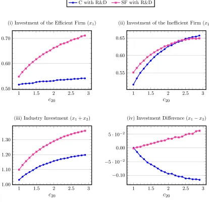
Figure 1.Investments Under the Two Forms of Competitions (C & SF)

1 1.5 2 2.5 3 0.50

0.60 0.70

c

(i) Investment of the Efficient Firm (x1)

C with R&D SF with R&D

1 1.5 2 2.5 3 0.55

0.60 0.65

c

(ii) Investment of the Inefficient Firm (x2)

1 1.5 2 2.5 3 1.00

1.10 1.20 1.30

c

(iii) Industry Investment (x1+x2)

1 1.5 2 2.5 3

−0.10

−5·10−2 0.00 5·10−2

c

(iv) Investment Difference (x1−x2)

higher than that of the inefficient firm under the supply function competition while the opposite becomes true under the Cournot competition.

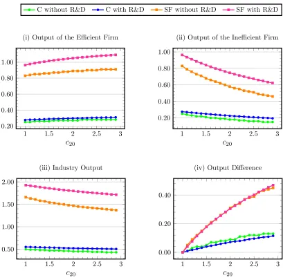
In Figure 2, we plot the equilibrium outputs both in the presence and absence of R&D. Note that an equilibrium with no R&D can arise in our model when the firms have no access to the R&D technology in equation (2) or when R&D is infinitely costly, i.e. δ=∞in equation (3). The first three panels of Figure 2 show that the outputs of both firms as well as the industry output are higher when investment in R&D is present than when it is not. However, the positive effect of R&D seems to be much more significant under the supply function competition than under the Cournot competition.

Figure 2.Comparisons of Outputs Under the Two Forms of Competitions (C & SF)

1 1.5 2 2.5 3 0.20

0.40 0.60 0.80 1.00

c

(i) Output of the Efficient Firm

C without R&D C with R&D SF without R&D SF with R&D

1 1.5 2 2.5 3 0.20

0.40 0.60 0.80 1.00

c

(ii) Output of the Inefficient Firm

1 1.5 2 2.5 3 0.50

1.00 1.50 2.00

c

(iii) Industry Output

1 1.5 2 2.5 3 0.00

0.20 0.40

c

In panels (i) and (ii) of Figure 2 we also observe that the effect of cost asymmetry on output is different for the two firms. For both types of competitions, this effect is positive for the efficient firm and negative (and much larger) for the inefficient firm, irrespective of the presence of R&D possibility. In fact, the said negative effect on the output of the inefficient firm is so large that the industry output is always decreasing in the level of cost asymmetry, as we observe in panel (iii). In addition, we observe in the first three panels that the effect of cost asymmetry becomes always more pronounced when the firms compete in supply functions. Finally, panel (iv) shows that the efficient firm always produces more than the inefficient firm under both types of competitions irrespective of whether the two firms are able to engage in R&D or not. Moreover, the difference between the firms’ outputs is always higher under the supply function competition than under the Cournot competition, while this difference is not affected by the possibility of R&D investment much.

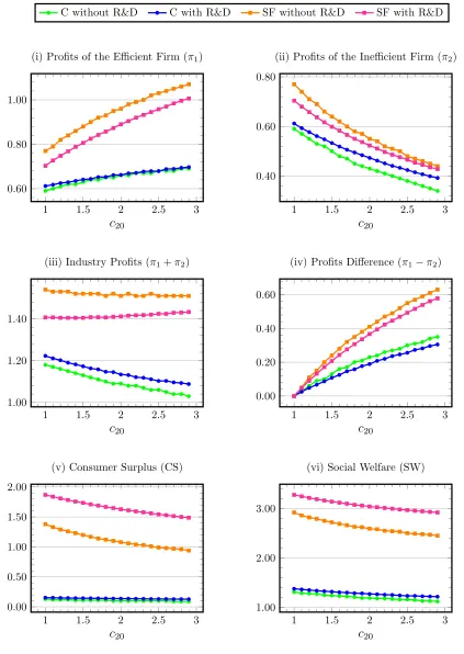
Next, in Figure 3 we plot the equilibrium welfares of producers, consumers, and the society as a whole. Panels (i), (ii), and (iii) illustrate the effects of R&D on the profits of the duopolists and the industry as a whole. While this effect is found to be always positive under the Cournot competition, it is always negative under the supply function competition. This latter negative effect is caused by the aggressive investment in R&D, especially by the efficient firm, observed under the equilibrium of the supply function competition (Figure 1), raising the industry output, and consequently reducing the product price, to a harmful level for both firms. Moreover, as expected, an increase in the cost asymmetry has a positive effect on the welfare of the efficient firm and a negative effect on the welfare of the inefficient firm under both types of competitions, irrespective of the presence or absence of R&D. However, which of these opposite effects becomes dominant on the total industry profits is more involving. As illustrated in panel (iii) of Figure 3, when the firms engage in the Cournot competition in the output market, the industry profits are decreasing at all levels of cost asymmetry irrespective of the possibility of R&D investment. On the other hand, when the firms compete in supply functions in the output market, the industry profits are always slightly decreasing with respect to the cost asymmetry in the absence of R&D and always slightly increasing in the presence of R&D. We also observe in panel (iv) that the firm that has an initial cost advantage in production can always obtain higher profits irrespective of the type of competition, the level of cost asymmetry, and the possibility of R&D investment.

Figure 3.Comparisons of Welfares Under the Two Forms of Competitions (C & SF)

1 1.5 2 2.5 3 0.60

0.80 1.00

c

(i) Profits of the Efficient Firm (π1)

C without R&D C with R&D SF without R&D SF with R&D

1 1.5 2 2.5 3 0.40

0.60 0.80

c

(ii) Profits of the Inefficient Firm (π2)

1 1.5 2 2.5 3 1.00

1.20 1.40

c

(iii) Industry Profits (π1+π2)

1 1.5 2 2.5 3 0.00

0.20 0.40 0.60

c

(iv) Profits Difference (π1−π2)

1 1.5 2 2.5 3 0.00

0.50 1.00 1.50 2.00

c

(v) Consumer Surplus (CS)

1 1.5 2 2.5 3 1.00

2.00 3.00

c

4

Conclusion

In this paper we have considered a duopolistic model with cost asymmetry to study how process R&D may affect the welfares of producers, consumers, and the society as a whole when both firms compete either in supply functions or in quantities in the output market. To this end, we have constructed a two-stage perfect-information game where the duopolistic firms non-cooperatively choose in the first two-stage their R&D investments and in the second stage their productions (according to the supply function or quantity competition). Solving the subgame-perfect Nash equilibrium of this game numerically for a wide range of initial cost parameters, we have found that under both types of competitions the outputs of both firms, and resultingly the industry output, are always higher when they both invest in R&D than when neither of them makes any investment.

We have also observed that the output expansion due to the aggressive R&D investment under the supply function competition becomes so large that the negative effect of this expansion on the profits of the firms and the whole industry outweighs a positive effect stemming from the reduction in the unitary marginal costs of the firms due to R&D. Consequently, under the supply function competition with process R&D the duopolistic firms find themselves trapped in a situation like the Prisoners’ Dilemma. Even though R&D can be beneficial for any firm when the rival firm has no access to R&D, it becomes destructive under the supply function competition when both firms non-cooperatively engage in R&D. In contrast, competing in R&D before the Cournot competition in the output market becomes always beneficial for both firms, especially for the inefficient firm. On the other hand, regarding the welfares of consumers and the society as a whole, we have found that R&D has always a positive effect under both types of competitions, whereas this effect is incomparably larger under the supply function.

Our simulations have also showed that the supply function competition is always Pareto superior to the Cournot competition at all levels of cost asymmetry, irrespective of the presence or absence of R&D. Besides, the possibility of R&D competition before the supply function competition in the output market may yield huge welfare benefits for consumers at the expense of huge profit losses for the duopolistic firms. This suggests that public authorities acting on behalf of consumers, or the society as a whole, may have strong incentives to subsidize (or facilitate) non-cooperative R&D investments of the duopolistic firms –at any level of cost asymmetry– when they compete in supply functions, like they usually do in electricity markets. Our findings also imply that social gains from such subsidies might be very small when the duopolistic firms compete in quantities.

References

Bertrand J (1883) Th´eorie math´ematique de la richesse sociale. Journal des Savants 67, 499–508.

Cournot A (1838) Recherches sur les Principes Mathematiques de la Theorie des Richesses. Paris: Hachette.

D’Aspremont C and Jacquemin A (1988) Cooperative and noncooperative R & D in duopoly with spillovers. The American Economic Review 78:5, 1133–1137.

Green R (1999) The electricity contract market in England and Wales. 47:1, 107–124.

Hinloopen J and Vandekerckhove J (2009) Dynamic efficiency of Cournot and Bertrand competition: input versus output spillovers. Journal of Economics 98:2, 119–136.

Klemperer PD and Meyer MA (1989) Supply function equilibria in oligopoly under uncertainty. Econo-metrica 57:6, 1243–1277.

Nash JF (1950) Equilibrium points in n-person games. Proceedings of the National Academy of Sciences 36:1, 48–49.

Qiu LD (1997) On the dynamic efficiency of Bertrand and Cournot equilibria. Journal of Economic Theory 75:1, 213–229.

Saglam I (2018a) The desirability of the supply function competition under demand uncertainty. Eco-nomics Bulletin 38:1, 541–549.

Saglam I (2018b) Ranking supply function and Cournot equilibria in a differentiated product duopoly with demand uncertainty. Available at SSRN: https://ssrn.com/abstract=3149142 or http://dx.doi.org/ 10.2139/ssrn.3149142.

Selten R (1965) Spieltheoretische Behandlung eines Oligopolmodells mit Nachfragetr¨agheit. Zeitschrift far die gesamte Staatswissenschaft 121, 301–324; 667–689.

Singh N and Vives X (1984) Price and quantity competition in a differentiated duopoly. Rand Journal of Economics 15:4, 546–554.

Symeonidis G (2003) Comparing Cournot and Bertrand equilibria in a differentiated duopoly with product R&D. International Journal of Industrial Organization 21:1, 39–55.