Measuring Tail Dependence for Aggregate Collateral
Losses Using Bivariate Compound Shot-Noise Cox
Process
Jiwook Jang1, Genyuan Fu2
1Department of Applied Finance & Actuarial Studies, Faculty of Business and Economics, Macquarie University, Sydney, Australia
2Benelec Pty Ltd., Sydney, Australia
Email: [email protected], [email protected]
Received October 4, 2012; revised November 4, 2012; accepted November 11, 2012
ABSTRACT
In this paper, we introduce tail dependene measures for collateral losses from catastrophic events. To calculate these measures, we use bivariate compound process where a Cox process with shot noise intensity is used to count collateral losses. A homogeneous Poisson process is also examined as its counterpart for the case where the catastrophic loss fre-quency rate is deterministic. Joint Laplace transform of the distribution of the aggregate collateral losses is derived and joint Fast Fourier transform is used to obtain the joint distributions of aggregate collateral losses. For numerical illustra-tions, a member of Farlie-Gumbel-Morgenstern copula with exponential margins is used. The figures of the joint distri-butions of collateral losses, their contours and numerical calculations of risk measures are also provided.
Keywords: Aggregate Collateral Losses; Bivariate Compound Cox Process; Shot Noise Process;
Farlie-Gumbel-Morgenstern Copula; Tail Dependence; Joint Fast Fourier Transform
1. Introduction
Over the recent years, numerous papers have looked at the modelling of dependence within an insurance port- folio or between insurance portfolios [1-5]. Also in the field of financial risk management, a range of papers on dependence modelling within credit risk and operational risk can be noticed [6-8]. Besides the construction of specific multivariate models, considerable attraction is given to the use of copulas. In particular, within the theory of Lévy processes, Lévy copulas have proven to be useful [9].
Our paper is very much based on insurance applica- tions where two lines of business are hit by a common external event, hence the word “collateral losses” in the title. These joint losses may, for instance be triggered by events such as flood, windstorm, hail, bushfire, earth- quake and terrorism. Particular examples concern colla- teral losses due to 2011 Great Eastern Japan Earthquake, 2010-2011 Queensland floods, 2009 Victorian Bushfires [10], 2005 Hurricane Katrina [11] and 2001 September 11 attack [12].
For the purpose of this paper, we concentrate on a very specific model and show how, within this model several explicit calculations for relevant risk quantities can be performed. The bivariate model we consider has the
following structure:
1 2
1 1
,
t t
N N
t i t
i i
L X L
Yi, (1)where k is the total loss arising from risk type
t
L 1, 2
k and t is the number of collateral losses up to
time . The random variables i
N
t X and Y ii, 1, 2,,
1
t
L 2
t
L N
denote the individual loss amounts. In this model, the de- pendence between two random variables and comes from the common arrival process t, together
with the dependence between the individual losses Xi and i. The latter is modelled using the notion of copula
[13]. To be more specific, we assume the loss random variable i
Y
X and Yi are independent identically distri-
buted with continuous distribution function FX and FY respectively. The joint distribution of the vector
X Y,
is assumed to be of the form with a given copula . The uniqueness of this two stage construction goes back to Sklar’s Theorem.
C FX,FY C
Theorem 1.1. (Sklar’s Theorem) Let F be a joint
distribution function with margins FX and FY. Then there exists a copula C such that for all x y, in
,
,
,
X
, Y
.If the margins are continuous, thenCis unique; other- wise C is uniquely determined on RanFXRanFY ,
where RanFiFi
denotes the range of Fi. Con- versely, if C is a copula and FX and FY are uni-variate distribution functions, then the functionFdefined in (2) is a joint distribution function with margins FX
and FY.
Proof. See Schweizer and Sklar [14] or Nelsen ([13], p. 18).
To deal with stochastic nature of catastrophic loss arrival in practice, we use a Cox process for t. The
Cox process provides flexibility by letting the intensity not only depend on time but also allowing it to be a stochastic process. Therefore the Cox process can be viewed as a two step randomisation procedure. A process
t
N
is used to generate another process t by acting its intensity. That is, t is a Poisson process conditional
on
N N
t
which itself is a stochastic process.
Losses arising from a catastrophe depend on its inten- sity. One of the processes that can be used to measure the impact of catastrophic events is the shot noise process. Previous works of insurance application using shot noise process and a Cox process with shot noise intensity can be found in [15-19]. Reference [20] also used a Cox process with shot noise intensity to model operational risk. The shot noise process is particularly useful to loss arrival process as it measures the frequency, magnitude and time period needed to determine the effect of cata- strophic events. As time passes, the shot noise process decreases as more and more losses are settled. This de- crease continues until another event occurs which will re- sult in a positive jump in the shot noise process. There- fore the shot noise process can be used as the parameter of a Cox process to measure the number of catastrophic losses, i.e. we will use it as an intensity function to generate a Cox process. We will adopt the shot noise process used by Cox & Isham [21]:
0
1
e t Mt e t Si
t i
i
Z
where:
0 is the initial value of t that is carried on from catastrophic events incurred previously;
Zi i1,2, is a sequence of independent and iden- tically distributed random variables with distributionfunction and (i.e. magni-
tude of contribution of catastrophic event to inten- sity);
0
G z z E Z
i
Si i1,2, is the sequence representing the event times of a Poisson process Mt with constant inten-sity ; and
is the rate of exponential decay.
Catastrophic events may take long to materialise so the
decay rate may not be exponential. It is assumed to be of this form for a matter of convenience, i.e. closed-form expressions of final results are easily derived. We also make the additional assumption that a Poisson process
t
M and the sequences
Zi i1,2,,
Xi i1,2, and
Yi i=1,2, are independent of each other.A Poisson process with loss frequency rate is also st
alculate the fo
udied for Nt, that may be considered when cata-
strophic loss f uency rate is deterministic. With the above model specifications, we c
req
llowing relevant risk measures:
1 2
1 1 2 1 1
lim ,
t t
t L t L
u L F l L F l
(3)
1 2
1 1 1 , 2 1 ,
t t
t t L t L
L L F l L F l
(4)
1 1
1 1 1 2 1
1 lim
t t
t L t t L
u L F l L L F l
Lt2 (5)
and
1 2
1 1 2 1 .
t t
t t t L L
L L L F l
(6)
Here 1
t
L
F , 2
t
L
F and 1 2
t t
L L
F
are the distribution fun s of the rando variab
easures, we need to ob
ction m les L 1 , L 2 and
t
(3) and (5t 1 2
t t
L L respectively. The quantities ) are asymptotic upper tail dependence measures and the quantities (4) and (6) are conditional tail expecta- tions. The motivation for calculating these quantities that measure extremal dependence in the upper tail of a bi- variate distribution is that insurance industry is more concerned with dependence between extreme losses. For a discussion on the coefficient of tail dependence para- meters, see McNeil et al. [22].
In order to evaluate above risk m known as
tain the joint distribution of the aggregate collateral losses L t1 and
2
t
L . Unfortunately, it is not easy to derive joint di tribution the aggregate collateral losses explicitly. So in Section 2, we derive joint Laplace transform of the distribution of the aggregate collateral losses expressed with a copula function applying the piecewise deterministic Markov processes (PDMPs) theory. For Nt, a shot-noise Cox process and a homo-
geneous Pois process are used respectively. Section 3 provides the expressions of the moments, covariance and linear correlation between 1
t
L and 2
t
L at time t for both cases. In Section 4, we present t expressions for joint probabilities of the aggregate collateral losses and their densities at 1 0
t
L
the s
son
he
and 2 0
t
L , which are re- quired to improve t racy of the distributions of the aggregate collateral losses inverting joint Fast Fourier transforms. We also provide the figures of the joint dis-
tribution of the aggregate collateral losses and their con- tours. In Section 5, we illustrate the calculations of rele- vant risk measures (3)-(6) using joint Fast Fourier trans- forms. For numerical illustrations, an exponential dis- tribution for the jump sizes of catastrophic event, a mem- ber of Farlie-Gumbel-Morgenstern copula with exponen- tial margins are used throughout the paper. Section 6 shows the sensitivity analysis on the parameters of a shot-noise Cox process from a Poisson process using the risk measure of (4). Concluding remarks are in Section 7.
2
.
Joint Laplace Transform of the
llateral
Th se deterministic Markov processes theory
2.1. Shot-Noise Cox Process
process follows a
Distribution of the Aggregate Co
Losses
e piecewideveloped by Davis [23] is a powerful mathematical tool for examining non-diffusion models. From now on, we present definitions and important properties of 1
t
L and 2
t
L with the aid of piecewise deterministic Marko pro- es theory [16,24,25]. This theory is used to derive joint Laplace transform of the distribution of the aggre- gate collateral losses 1
t
L and 2
t
L .
v cess
Assuming that the loss arrival Nt
Cox process with shot noise intensity t, t e generator
of the process
, , , 1, 2,
acting on a func- ht t N L Lt t t t
1 2
tion f
, , ,nl ,l ,t
belonging to its domain is given by
1 2 1 2 0 0 2 1 21 2 1 2
0
, , , , ,
, , 1, , ,
,
d d
, , , , ,
, , , , , d , , , , ,
Af n l l t
f f
t
f n l x l y t
C F x F y x y x y
f n l l t f
f z n l l t G z f n l l t
(7) where 0 d t t s s
. Now let us find a suitable martingalein order to derive joint Laplace transform of the dis-
Lemma 2.1. Considering constants
tribution of the aggregate collateral losses 1
t
L and 2
t
L .
0 1, 0, 0 and0 then
1 2 0 exp exp ˆexp , 1
ˆ
exp e exp 1 e d
t N t t t t t s t L L c g s
(8)martingale, where is a
x y2C
0 0
,
, e e F x F y d d
c x y
x y
ˆ
and
ˆ
0 e duz
g u G
z .Proof. From (7), f
, , , n l 1,l2,t
has to satisfy 0f
A for f
, , n l, 1,l2,t
to be a martingale. Setting
1 2 1 2 , , , , ,e exp exp exp e eB t
n t
n l l t
l l f
we get the equation
ˆ
, 1
gˆ
et 1
B t c 0 (9)
e solution is
s (10)
ich the result follows.
ined in Lemma 2.1 and sett- and th
by wh
ing
d
0
ˆ , 1 , 1 ˆ e d
t
s
c B t g
Using the martingale obta 1
and 0, we can easily obtain the general form int Laplace transform of the distribution of the aggregate collateral losses 1
t
L and 2
t
L , i.e.
of jo
1 2 L L 2 2
2 1 1 1 1 2 e e ˆ
p exp exp , 1 d ,
t t t t s t t t
L L c s
(11)where the conditional expectation is based on the ex
E
E
probability space
, ,P
, and t information set he
t t0 with the filtration
t s L Ls s s t
1 2
, , :
. Without loss of generality,
he time scale an
change t d assume that L 1 0
0 and
2 0 0,
L then it is given by
1 2
0
0 ˆ
e t e t exp , 1 d .
t L L
s
E c s
(12). If loss X sizes of catastrophic event follow an exponential distri-
bution, i.e. g z
exp
z z
, 0, 0 and that tis stationary [16], (12) i
given by
. Then using Theorem 2.6 in s
occurs by arriva noise in ity
1 2 ˆ 1 , e e e ˆ 1 , 1 e ˆ 1 , 1 e . e t t t L L t c t t E c c (13)Secondly, as a specific example for , we use the
Fa as
4) where
C
rlie-Gumbel-Morgenstern (FGM) copul given by
,
1
1
,C u v uvuv u v (1
0,1 ,
0,1 and
1,1
u v .
his calculation somewhat easier, w
1 ey 0,y 0
it th
as
e co L
rrespond- ing expression for the above
astly, to
make t e sume that
1 e x
0, 0
F x x and . We om
F y
joint Laplace transform of the distribution of the aggregate collateral losses as it can be easily obtained using the joint distribution function
,F x y driven by (14), i.e.
ˆ , 2 2 1 . 2 2c
(15)
It will be of interest to examine the joint Laplace trans- form of the distribution of the aggregate collateral losses
1
t
L and 2
t
L at time t, using other copulas and other
gins
mar F x
and F y
. If
Zi i1,2,, which are the magnitude of contribution of catastrophic event to inten- sity t, are high, we also need to consider heavy-tailed distri tions for jump size of catastrophic event, bu G z
. We also omit the corresponding expressions f Laplace transform of the distribution of i, 1, 2t
L i which are the Laplace transforms of the distr
the compound Cox process with shot noise intensity t or the
ution of ib
, where its jump sizes follow an exponential distribut [16].
If w
ion
e set 0 istribu
in (15), we have joint Laplace trans- form of the d tion of the aggregate collateral losses, which is the case that two losses X and Y occur same time from a sharing loss frequency rate t, but their sizes are independent each other. Due to the ependence of collateral losses of X and Y with sharing loss fre- quency rate t
d
, we can see that
1
2e t e t e Lt e Lt
E L1 L2 E E (16)
even if 0 l process
1
t
N with shot tens 1
t
that has three para- meters of 1, 1 and
z 1 and loss Y occurs byal process N 2 with sho intensity 2
G
arriv t t noise t that
has three parameters of 2
,
2 and G z
2 and everything is inde ndent each other, we can e the joint Laplace transform of bution egate 1 2
pe hav
the distri of aggr
Let us now assume that the loss arrival process s with loss losses Lt and Lt at time t, that is the product of the
Laplace transforms of the distribution of i, 1, 2
t
L i .
2.2. Homogeneous Poisson Process
t
N
fre- follows a homogeneous Poisson proces
quency μ. Setting t in (12), i.e. considering det
ministic loss frequency μ, we can easily obtain that
er-
2
t
L
1
ˆ
e Lt e exp 1 ,
E c t (17)
and using (14) we have
1 2 e e 2 2 exp . 2 2 t t L L E t (18) We omit the corresponding expressions for the La- place transform of the distribution of , w ar i, 1, 2 t
L i
ntial los
hich e the Laplace transforms of the distribution of the compound Poisson process with expone s sizes, as they can be easily obtained setting 0 and 0, respectively.
Similar to shot-noise Cox process for Nt, due to the
dependence of collateral losses of X and Y
sh
with aring loss frequency rate , it shows th
at
1 2
1 2
e Lt e Lt e Lt e Lt
E E E
(19) even if 0. If loss X occurs by arrivalwith loss frequenc
process 1
t
N y 1 and loss Y occurs by
arrival process Nt with oss frequency
2 l 2 and
everything is independent eac other, we can also have the joint Laplace transform of the distribut of aggregate losses Lt and
2
t
L at time t that is the product of the Laplace transforms of the distribution of
i, 1, 2 t
L i .
3
oments, Covariance and Linear
hion 1
. M
Correlation of Aggregate Collateral
In nce and
Losses
linear correlation between 1 and at time . For
t
L 2
t
L t
the loss arrival process Nt, we use a Cox process with
shot noise intensity t an a hom eneous Poisson
process with loss frequency
d og
, respectively.
3.1. Shot-Noise Cox Process
Also set 0 and 0 in (12) and differentiate itw.r.t. v and respectively, we can obtain the expecta- tion of 1 and at time t, i.e.
t
L 2
t
L
1
t t
E L E E X (21) and
Differentiating (12) w.r.t. and and set 0 and
2
.
t t
E L E E Y (22) 0,
we can derive the joint e
2 xpectation of and
1
t
L
t
L at time t, i.e.
The higher moments of and at time t canbe obtained by differentiating it further, i.e. 1
t
L 2
t
L
.E L1 2
2
t Lt E t E XY E t E X E Y (20)
1
2
2t t t
Var L E E X Var E X (23) nd
a
2
2
2.t t t
Var L E E Y Var E Y (24) The covariance between and at time is given by
(25)
and the linear correlation coefficient between and at time is given by 1
t
L 2
t
L t
1, 2
t t t t
Cov L L E E XY Var E X E Y
1 2
t
L Lt t
1 2
2 2 2 2 2 2 2 2
,
t t
E t XY t E X E Y
t t t t
L L
E Var
E E X E Y E Var E X E Y E X E Y Var E X E Y
(26)
Let us now illustrate the calculations of the covariance nd linear correlation between and at time
1 2
2 .t t
E L L tE XY t E X E Y a
w
1
t
L 2
t
L t, here Nt follows a shot-noise Cox process.
Example 1
From [17], we have
2 2 2 3 2 32 2 e t 2
t t
(27)
r f vari
T een nd at e t is
given by
We omit the exp essions or the expectation and - ance of 1
t
L and 2
t
L at time t as they can be easily derived similar to a shot-noise Cox process for
he covariance b t
N . tim etw 1 a
t
L 2
t
L ,
t
E t Var
and using (14) we have
1 2
,
t t
Cov L L tE XY (28) and the linear correlation coefficient between 1 and
Lt
1 1 .4
E XY
The parameter values used to calculate the covariance and linear correlation using (25) and (26) are
2 at time t is given by
t
L
1 2
2 Y2
, .
t t
E XY L L
E X E
(29)
var
and and at time
where follows a Poisson
Exam e 2
0.5, 2, 1, 1, 0.5,t 1.
Hence from (25) and (26), the calculation
Let us now illustrate the calculations of the co iance linear correlation between 1
t
L process.
2
t
L t,
t
N
pl
s of cova- riance and linear correlation between and at tim
Similar to a shot-noise Cox process for differen- 1
t
L 2
t
L e t are shown in Tables 1 and 2 respectively. 3.2. Homogeneous Poisson Process
The parameter values used to calculate the covariance and linear correlation using (28) and (29) are
4, 1, 0.5,t 1.
From 8) and (29), the calculations ,
t
N
tiating (17) w.r.t. and and set 0 and 0 we can easily derive the joint expectation Lt , and
2
L at time t, i.e.
of 1
t
(2 ear correlati
of covariance and lin
sh
on between Lt and Lt at time t are
Table 1. Covariance between 1
t
L and L t
2.
θ Cov L Lt t
1, 2
−1 12.82
−0.5 13.82
15.82 0 14.82
0.5
[image:6.595.54.288.242.347.2]1 16.82
Table 2.Linear correlation between
1t and L L t
2.
θ
1, 2t t L L
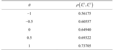
−1 0.56175
−0.5 0.60557
2 0 0.64940
0.5 0.6932
1 0.73705
Table 3. Covariance between
1t
L and L t
2.
θ
1, 2t t v L L Co
−1 6
−0.5 7
0 8
0.5 9
1 10
Table 4.Linear correlation between 1 and
t
L L t
2
.
θ
1, 2
t t L L
−1 0.375
−0.5
0
0.4375
0.5
0.5 0.5625
1 0.625
3.3. Comparison
The paramet alues used in Examples 1-2 ovide us with the sam means of aggregate collateral losses regardless of t ss arrival process i.e.
where
er v e
pr
he lo Nt,
Poisson k Cox k ,
t t
L L
1 Poisson (1) Cox 4t t
L L
(30)
and
2
2 Poisson Cox 8.t t
L L
(31)
ever for each
How ,
om ocess.
n be om
Tables 1 and 3 show that there is an increase in the covariance between
by changing fr a homogenous Poi t-noise C pr Tables 2 and 4 h
the linear co tween and incre
by changing fr a homog s Poi a shot-noise
1
t
L sson also s
2
t
L sson p
and 2
t
L process to
t
N ox rrelatio
t
N
a sho ow that
ases 1
t
L
enou rocess to
Cox process for each . This implies that the marginal distributions of the aggregate collateral loss with respect to a Cox process have heavier tail than their counterparts with respect to a Poisson process, i.e.
1 1Poisson 8 C 41
t t
Var L Var L (32)
and
ox 11.
2
2Poisson 32 Cox 45.64.
t t
Var L Var L (33)
It will also become apparent by the joint distributions of aggregate collateral losses and their contours
tion 4 and numerical risk measure values in Exa
4. Joint Distribution of the Aggregate
t bivariate Fast Fourier transforms from joint Laplace transforms of the vector
in Sec- mples 3- 6.
Collateral Losses via Bivariate Fast
Fourier Transform
In order to calculate the risk measures of (3)-(6), we in- ver
1, 2
t t
L L
5,
obtained in Section er trans-
fo calcula-
tio we present the ex-
2. For details on how to use bivariate Fast Fouri rm, we refer to [26-28]. Before we show the
ns of risk measures in Section
pressions for the joint probabilities of the aggregate collateral losses and their densities at 1 0
t
L and
2 0
t
L . These are required to im rove the accuracy of the joint distributions of the aggregate collateral losses inverting bivariate Fast Fourier transforms.
4.1. Shot-Noise Cox Process If we let
p
and in (13), w e the
on for the joint probability of aggregate collateral losses at 1 0
t
L
e hav expressi
and 2 0
t
L , i.e.
1 1 2 e
0, 0
1 e
t t
L L
t .
(34) t
Regardless of loss size distributions, we have the same joint probability of aggregate collateral losses at 1 0
t
L
and L 2 0
t
process
wh loss ar
a Cox with shot noise intensity
en the rival process Nt follows
t
ˆ 1 , , 1 e ˆ 1 , 1 e c t t c 1 , e e lim ,e 1 e
t t t t
the expression for the joint density of aggregate collateral losses at ˆ 1 c
1 0
t
L and L t2 0 is given by
1
, 0, 0 e ln 1 e 1 .
1 1 e 1 e 1 e
t t
X Y
t t t
f
et
(35)
ss sizes (14), i.e
Based on (35), we can easily obtain its expression for exponential lo using .
1
1 e 1 e 1
ln .
1 1 e 1 e 1 e
t t
t t t
et
(36)
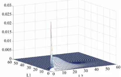
Figures 1-4 are the joint distributions of aggregate 4.2. Homogeneous Poisson Process
f
collateral losses and their contours at each value of If we let and in (18),
expression for the joint probability of aggreg losses at
we have the ate collateral with respect to a shot-noise Cox process for
Figure 2 (or Figure 1) shows that joint pr ilities o ggregate collateral losses are mainly located between
t
N . obab
1 0
t
L and 2 0 i.e.
t
L , a
the bottom left corner and the top right corner when 1
, which means loss X and Y move in the same direction. On the other hand, compared to when 1,
Fi
L1 0,L2 0
e t. t t (37)
Regardless of loss size distributions, we have the same ability of agg egate co sses at 1 0
gure 4 (or Figure 3) shows that joint probabilities of aggregate collateral losses at the bottom left corner and the top right corner moves to its diagonal left and right, respectively when 1 which means loss X and
Y move in the opposite direction.
t
L
joint prob r llateral lo
and L 2
t
N follows 0
t
ogeneo
wh loss ar
a hom us Poisson process with loss en the rival process
frequency . If we set
, lim exp 2 expression for the joint density of aggregate collateral
sses at and is given by
2 e , 2 2 t t th lo e
1 0
t
L 2 0
t
L
, 0, 0 e .
t X Y
f t (38) Based on (38), we can easily obtain its expression for exponential loss sizes using (14), i.e.
1
te .t (39)The figures of the joint distribution co
s of aggregate llateral losses and their contours at each value of with respect to a Poisson process for are omitted, for which see the early version of this paper in Nt
http://ssrn.com/author=383758.
1-2 and alculations of the risk
measures of (3)-(6) with respect to a shot-noise Cox process and a Poisson process. They are shown in Tables 5-18.
To reduce the error of used algorithm for inverting bivariate Fast Fourier transforms using Matlab, the fol- lowing methods have been used:
e
5
.
Calculating
Risk Measures for Collateral
Losses
Now using the parameter values in Examples
Matlab, let us illustrate the c
The sampling points have been taken as many as possible, i.e. we have used 8192 × 4096 points in th calculation, which was the maximum points we could sampled in 32-bit Matlab.
If the sampling interval gap is too small, there would be a large amount of truncation error. Also if the sampling interval is too big, there would be a large
.
amount of sampling error. Hence we have chosen carefully the right sampling interval, so that the total errors caused by inverting bivariate Fast Fourier transforms could be negligible
Figure 1. The joint distribution of collateral losses with θ = 1.
Figure 2. The contour of the joint distribution of collateral losses with θ = 1.
Figure 3. The joint distribution of collateral losses with θ =
−1.
low-pass/moving-average filter to filter the jitter noise out. Then we have used the linear interpolation to smooth the borders of the data. The pattern matrix used for this filter was
0.0625 0.125 0.0625 0.125 0.25 0.125 0.0625 0.125 0.0625
.
Figure 4. The contour of the joint distribution of collateral losses with θ = −1.
Example 3
Using the different at and
the calculations of th
Tables 5-8.
Tables 5-8 show that each quantile values are higher with respect to a shot-noise Cox process than their counterparts. They also show that the risk measures of (3) with respect to a shot-noise Cox process are higher than
e aggregate collateral losses with re- -noise Cox process have heavier tail than
th respect Poisson pro
%
q
VaR
e risk
% 95%
q
measure of (3) are shown i 99%,
n
their counterparts. These justify that the marginal/joint distributions of th
spect to a shot
eir counterparts with to a cess.
Example 4
Secondly, based on the VaRq% at 95% and 99% in Example 3, the calculations of the risk measure (4), i.e.
1 2
1 1 1 , 2 1
t t
t t L t L
L L F u L F u
are shown in Ta-
bles9 and 10.
Tables 9 and 10 show that the risk measures of (4)
with respect to a shot-noise Cox process are higher than their counterparts regardless of the critical values. Re- gardless of the loss arrival process Nt, the risk measures
of (4) are getting bigger as the critical value goes to 99%.
Th rences
9
Example 5
ey also show that the diffe between the values in
Table 9 and their counterparts in Table 10 are getting higher as the critical value goes to 9 %.
Showing the calculations of the q% quantiles of the sum, 1 2
t t
L L , i.e. 1 2
t t
L L
1
F u
in
1 2
1 2 > 1
t t
t t L L
L L F u
and the joint probability be-
tween 1
1 1
t
t L
L F u and
1 2
1 2 1 ,
t t
t t L L
L L F u
i.e.
1 1 2
1 1 , 1 2 1
t t t
t L t t L L
L F u L L F u
for each cases
in Tables11-14, the calculations of the ris e shown in T
k measure (5)
[image:8.595.67.285.453.598.2]
1 10.55
2 21.10
0.05t t
L L
[image:9.595.56.539.111.214.2] .
Table 5. A shot-noise Cox process, where
1 10.55, 2 21.10
t t
L L
1 10.55 2 21.10
2 21.10 1 10.55
t t t t
L L L L
0.02090
1 0.41793
0.5 0.019
0.015
00 0.38002
0 0.01723 0.34449
0.5
55 0.31105
1
[image:9.595.57.539.249.350.2] 0.01397 0.27946
Table 6. A Poisson process, where
1
2
9.37 18.74 0.05
t t
L L
.
1 9.37, 2 18.74
t t
L L
1 9.37 2 18.74
2 18.74 1 9.37
t t t t
L L L L
1 0.01459 0.29186
0.5 0.012
0.008
0.146
57 0.25129
0 0.01068 0.21363
0.5
93 0.17862
1
[image:9.595.54.542.387.487.2] 0.00730 05
Table 7. A shot-noise Cox process, where
L t
L t
1 2
14.79 29.58 0.01 .
1 14.79, 2 29.58
t t
L L
1 14.79 2 29.58
2 29.58 1 14.79
t t t t
L L L L
1 0.00284 0.28389
0.5 0.00247 0.24727
0 0.002
0.001
0.156 14
84
0.21401
0.5
0.18373
1
[image:9.595.59.538.522.623.2] 0.00156 17
Table 8. A Poisson process, where
1 12.61
2 25.22
0.01t t
L L
.
1 12.61, 2 25.22
t t
L L
1 12.61 2 25.22
2 25.22 1 12.61
t t t t
L L L L
1 0.00152 0.15183
0.5 0.00121 0.12079
0 0.000
0.000
0.050 94
70
0.09369
0.5
0.07022
1
0.00050 13
θ q% 95%
Table 9. A shot-noise Cox process.
[image:9.595.308.537.650.736.2]99%
Table 10. A Poisson process.
θ q% 95% 99%
1 13.99969 18 8178.1 1 11.89360 14.99842
0.5 1
1
3.99910 18 7480.1 0.5 11.85723 14.95484
0 11.80964
0 13.98970 18 87 14.90020
0.5
.158
11.74893 14.83189
0.5
3.97155 18.13402
1
Table 11. quantiles of the s for a hot- noise Cox p ess.
θ q 99%
%
q um, L t L t
1 2 s
roc
% 95%
1 30.27695 41.70510
0.5 30.04685 41.32161
0 29.81675 40.93811
0.5
29.58665 40.59297
1
[image:10.595.54.541.157.743.2] 29.35656 40.17112
Table 12. q% quantiles of the s for a pois-
θ q% 95% 99%
um, L t L t
1 2
son process
1 26.44199 34.68714
0.5 26.17355
25.90510 34.22695
0 33.80510
0.5
25.63665 33.30656
1
25.32986 32.80801
Table 13.
>
, >F 1
u
1 1 1 2 1
t t
t L t t L
L F1 u L for a
shot-noise Co
t
L2
x process.
L
θ q% 95% 99%
1 0.02942 0.00469
0.5 0.02798 0.00439
0 0.026
0.003
57 0.00410
0.5
0.02519 0.00380
1
0.02384 54
Table 14.
>
, >
t t
t L t t L
L F u L F u
1 11 1 2 11
t
L2 for a
ss.
θ q% 95% 99%
L Poisson proce
1 0.02444 0.00344
0.5 0.02264 0.00311
0 0.02085 0.00275
0.5
0.01906 0.00243
1
0.01736 0.00210
> >
t t
t L t t L
L F u L
Table 15.
t
L
F u
1 1 2
1 1 1 2 1 for a
θ q% 95% 99%
L shot-noise Cox process.
1 0.58843 0.46900
0.5 0.55950 0.43908
0 0.53137 0.40990
0.5
0.50387 0.38020
1
0.47681 0.35389
Table 16.
>
t
t L >
t t
t t L L
L F
1 u L L F 1 2 u
1 1 1 2 1 for
a Poisson pr ess.
θ q 99%
oc
% 95%
1 0.48882 0.34377
0.5 0.45288 0.31048
0 0.41706 0.27504
0.5
0.38126 0.24282
1
0.34710 0.21026
θ q% 95%
Table 17. A shot-noise Cox process.
99%
1 11.69317 14.99356
0.5 11.46820 14.64166
0 11.22903 14.25449
10.97467 0.5
13.75803 1
10.70397 13.36212
Table 18. A Poisson process.
θ q% 95% 99%
1 9.57781 11.53855
0.5 9.28678 11.14740
0 8.96709 10.60372
0.
5 8.61560 10.13953
1
Tables 11 and 12 show that the quantiles the sum, with respect to a se Cox process
are rdless of the
critical v l process
they g bigger al oe
how that the differe ces betwee values in ble 11 and their counterparts in Table are getting higher as the critical valu es to 99.9%.
Tables 13 and 14 show that e joint probability be-
tween and with
respect to a Cox process are higher than r counterparts regardless of the critical values. Reg less of the loss rrival process , they are getting smaller
as The
ferences
of
Example 6
% q ot-noi
e critical v n
of 1 2
t t
L L higher than
alues. a
. They also s
sh a
their counterp rts rega
Regardless of the loss arriva Nt,
s to n the
re gettin as th ue g
99.9%
Ta 12
e go th
1
1 1
t
t L
L F u
1 2 1
1 2
t t
Lt Lt
L L F u
shot-noise thei
ard
a t
the critical value goes to 99.9%. y also show that the dif between the values in Table 13 and their counterparts in Table 14 are getting lower as the critical value goes to 99.9%.
Tables 15 and 16 show that the risk measures of (5)
with respect to a shot-noise Cox process are higher than their counterparts regardless of the critical values. Re- gardless of the loss arrival process N , the risk m
N
t easures
(5) are getting smaller as the critical value goes to 99.9%.
Lastly, based on the quantile values and the joint probabilities in Example 5, the calculations of the risk measure (6), i.e.
1 2
1 1 2 1
t t
t t t L L
L L L F u
are
shown in Tables 17 and 18.
Tables 17 and 18 show that the risk measures of (6)
with respect to a shot-noise Cox process are higher than their counterparts regardless of the quantile values. Re- gardless of the loss arrival process Nt, the risk measures
of (6) are getting bigger as the critical value goes to 99.9%. They also show that the differences between the values in Table 17 and their counterparts in Table 18 are getting higher
With respect
as the critical value goes to 99.9%. to the FGM copula correlation parameter, , the risk measures of (3)-(6) are increasing (decreasing) as it changes to 1
1
be in g other cop
regardless of the loss arrival teresting to find these risk re va usin ulas with different marginal
t
process Nt. It will mea-
su lues distributions.
6
.
Sensitivity Analysis
In this section, we examine the effec on the risk measure of (4), i.e.
sh
w
1 2
1 1 1 , 2 1
t t
t t L t L
L L F u L F u
caused by changes in the values of the parameters of a ot-noise Cox process from a Poisson process. To do so,
e double the means of aggregate collateral losses, (30) and (31) with 8 for a Poisson case and with
4,
0.25 and 0.5, respectively for shot- noise Cox case, i.e.
1
1 Poisson Cox 8t t
L L
and
2
2 Poisson Cox 16,t t
L L
where other parameter values are the same as in Exam- ples 1-2.
Figures 5-6 are the joint distribution of aggregate
[image:11.595.311.535.480.704.2]collateral losses and its contour at 1 with respect to a Poisson process for Nt. Figures 7-12 are the joint dis- tributions of aggregate collateral losses and their con-
Figure 5. The joint distribution of collateral losses with θ = 1 for a Poisson process.
Figure 7. The joint distribution of collateral losses with θ = 1 and ρ = 4.
Figure 8. The contour of the joint distribution of collateral sses with θ = 1 and ρ = 4.
[image:12.595.58.286.285.512.2]lo
[image:12.595.320.527.330.462.2]Figure 10. The contour of the joint distribution of collateral losses with θ = 1 and δ = 0.25.
Figure 11. The joint distribution of collateral losses with θ = 1 and γ = 0.5.
Figure 12. The contour of the joint distribution of collateral losses with θ = 1 and γ = 0.5.
[image:12.595.319.525.508.705.2] [image:12.595.59.290.554.706.2]Table 19.
1 2( )
1 1 2 1
t t
t t t L L
L L L F u
.
1
%q A Poisson process A shot-noise Cox process 4
0.25 0.5
95% 18.52079 21.41422 21.37291 23.50179
99% 22.33392 26.15472 26.47892 29.68759
tours at 1 .
-12
with respect to a shot-noise Cox process for
(shot-noise Cox cases) show how dif- ferent joint probabilities of aggregate collateral losses are from Figures 5-6 (a Poisson case) by changes in the value of
t
N
Figures 7
, and
e same mean, th es for s
, respectively. Even though they have th e joint probabilities of aggregate collateral loss hot-noise Cox cases are located more between the bottom left corner and the top right corner when 1 than its counterpart. Shot-noise Cox
ases di have heavier tail than their
counterparts hown in Table 19 in terms of the risk (4). Compared to the effect on the
risk m ) by changes in the value of
c splay that they , which are s measure of easure of (4 , and
, respectively that
from a Poisson case, Table 19
shows , which is the parameter in exponential jump size distribution of catastrophic event, is the most sensitive parameter in terms of changes in the value the risk measure of (4).
7. Conclusions
We have used bivariate compound process to model aggregate collateral losses arising from catastrophic
er of collateral losses, a Cox process was sed to accommodate the stochastic nature of their fre- quency rate in practice. The shot noise s used as the intensity of a Cox process as the number of collateral lo ses rising from ents depends
on the frequency and magn mary events
and the time period needed to determine the effect of these events. o examined a Poiss process for the number of collateral losses as its counterpart. With the common collateral loss arrival process in the bivariate odel, the dependence between the individual losses
om d
not f copula where for numerical illustrations, a m
collateral
tween
surance premiums. We have presented the expressions for joint probabilities of the aggregate collateral losses and their densities at 1
0
t
L and , which were used to improve the of joi utions of the aggregate collateral losses inverting the Fast Fourier transforms. We have compared the simulated risk mea- sure values obtained using a compound Poisson and a compound shot-noise Cox model, respectively. The s
ess also provided using the isk measure of (4).
Other counting processes and other copulas with dif- ferent margins can be considered in the proposed bi- variate model, that we leave for further research. We hope that what we have presented in this paper provides practitioners with feasible models to quantify collateral losses that would occur more often due to global warm- ing, climate change and terrorism.
REFERENCES
[1] N. Bäuerle and A. Müller, “Modeling and Comparing Dependencies in Multivariate Risk Portfolios,” ASTIN Bulletin, Vol. 28, No. 1, 1998, pp. 59-76.
doi:10.2143/AST.28.1.519079 2
0
t
L
nt distrib accuracy
en-sitivity analysis on the parameters of a shot-noise Cox
rocess from a Poisson proc p
r
events such as flood, storm, hail, bushfire and earthquake.
For the numb [2] H. Cossette, P. Gaillardetz, E. Marceau and J. Rioux, “On
Two Dependent Individual Risk Models,” Insurance:
Mathematics and Economics, Vol. 30, No. 2, 2002, pp. 153-166. doi:10.1016/S0167-6687(02)00094-X
u
process wa
[3] C. Ge M. Mesfioui, “Compound Poisso with De- pendent Risks,” Insurance: Mathematics and Economics, Vol. 32, No. 1, 2003, pp. 73-91.
doi:10.1016/S0167-6687(02)00205-6
s a catastrophic ev
itude of the pri
We als on
nest, E. Marceau and
n Approximations for Individual Models
[4 N. Bäuerle and R. Grübel, “Multivariate Counti g Proc- esses: Copulas and Beyond,” ASTIN Bulletin, Vol. 35, No.
] n
m 2, 2005, pp. 379-408. doi:10.2143/AST.35.2.2003459 [5] M. L. Centeno, “Dependent Risks and Excess of Loss
Reinsurance,” Insurance: Mathematics and Economics, Vol. 37, No. 2, 2005, pp. 229-238.
doi:10.1016/j.insmatheco.2004.12.001
[6] F. Lindskog and A. J. McNeil, “Common Poisson Shock Models: Applications to Insurance and Credit Risk Mod- elling,” ASTIN Bulletin, Vol. 33, No. 2, 2003, pp. 209- 238. doi:10.2143/AST.33.2.503691
[7] D. Pfeifer and J. arising fr ifferent risk type has been modelled using
the ion o
ember of Farlie-Gumbel-Morgenstern copula with ex- ponential margins was used.
As it was difficult to derive the joint distributions the aggregate losses, we derived their Laplace transforms and inverted their Fast Fourier transforms numerically to calculate introduced relevant risk mea- sures. These measures can be used to calculate tail de-
Bulletin, Vol. 34, No. 2, 2004, pp. 333-360. doi:10.2143/AST.34.2.505147
[8] V. Chavez-Demoulin, P. Embrechts and J. Nešlehová, “Quantitative Models for Operational Risk: Extremes, Dependence and Aggregation,” Journal of Banking and Finance, Vol. 30, No. 10, 2006, pp. 2635-2658.
doi:10.1016/j.jbankfin.2005.11.008
[9] R. Cont and P. Tankov, “Financial Modelling with Jump Processes,” Champan & Hall, Boca Raton, 2004.
[10] Victorian Bushfires Royal Commission, “Final Report- Summary, Parliament of Victoria,” Parliament of Victoria, Melbourne, 2010.
[11] M. L. Burton and M. J. Hicks, “Hurricane Katrina: Pre- liminary Estimates of Commercial and Public Sector Damages,” Marshall University, Huntington, 2005. [12] G. Makinen, “The Economic Effects of 9/11: A Retro-
spective Assessment,” Congressional Research Service, Washington DC, 2002.
[13] R. B. Nelsen, “An Introduction to Copulas,” Springer- Verlag, New York, 1999.
[14] B. Schweizer and A. Sklar, “Probabilistic Metric Spaces,” Elsevier, New York, 1983.
[15] C. Klüppelberg and T. Mikosch, “Explosive Poisson Shot Noise Processes with Applications to Risk Reserves,”
Bernoulli, Vol. 1, No. 1-2, 1995, pp. 125-147. doi:10.2307/3318683
[16] A. Dassios and J. Jang, “Pricing of Catastrophe Reinsur- ance & Derivatives Using the Cox Process with Shot Noise Intensity,” Fi ce & Stochastics, Vol. 7, No. 1, 2003, pp. 73-95.
between Events of a Cox Process with Shot Noise Inten-sity,” Journal of Applied Mathematics and Stochastic Analysis, Vol. 2008, 2008, Article ID: 367170.
doi:10.1155/2008/367170
[19] J. Jang and Y. Krvavych, “Arbitrage-Free Premium Cal- culation for Extreme Losses Using the Shot Noise Proc- ess and the Esscher Transform,” Insurance: Mathematics and Economics, Vol. 35, No. 1, 2004, pp. 97-111. doi:10.1016/j.insmatheco.2004.05.002
[20] J. Jang and G. Fu, “Transform Approach for Operational Risk Management: VaR and TCE
tional Risk, Vol. 3, No. 2, 2008, pp.
45-,” Journal of Opera-
61.
and Tools,”
Prince-chastic Mod-
tical SocietySeriesB, Vol. [21] D. R. Cox and V. Isham, “Point Processes,” Chapman &
Hall, London, 1980.
[22] A. McNeil, R. Fr