J. Range Manage.
56:140-145 March 2003
A digital photographic technique for assessing forage utilization
P. W. HYDER, E. L. FREDRICKSON*, M. D. REMMENGA, R. E. ESTELL, R. D. PIEPER, AND D.M. ANDERSON
Authors are Senior Research Assistant and Research Scientist, USDA, Agricultural Research Service, Jornada Experimental Range, Las Cruces, N.M.
88003, associate professor, University Statistics Center, New Mexico State University, Research Animal Scientist, USDA, Agricultural Research Service, Jornada Experimental Range, Las Cruces, N.M. 88003, Professor Emeritus, Department of Animal and Range Sciences, New Mexico State University, and Research Animal Scientist, USDA, Agricultural Research Service, Jornada Experimental Range. *Corresponding author.
Abstract
Changes in forage utilization have been difficult to measure non-destructively without some level of subjectivity. This subjec- tivity, combined with a lack of reproducibility of visual estimates, has made forage utilization measurement techniques a topic of considerable discussion. The objective of this study was to devel- op and test the accuracy and repeatability of an objective, com- puter-based technique for measuring changes in plant biomass.
Digital photographs of target plants acquired before and after partial defoliation were analyzed using readily available image analysis software. Resulting data were used to develop a simple linear random coefficient model (RC) for estimation of plant bio- mass removed based on the area of the plant in the photo.
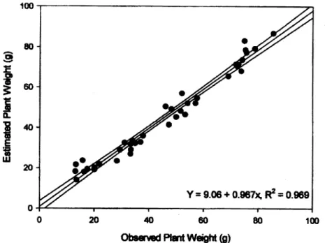
Sample collection took approximately 20 minutes/plant for alfal- fa (Medicago sativa L.). Analysis of images took another 60 to 90 minutes. Regression analysis gave an R2 of 0.969 for predicted vs.
observed plant weights. Testing this model using 10 alfalfa plants yielded weight estimates of defoliated plants accurate to within +/- 8.5%. The advantage of the RC model is its ability to use eas- ily obtained coefficients from simple linear regression models developed from each plant in a way that accounts for the lack of independence between samples within an individual plant. The technique described here offers an objective and accurate method for measuring changes in plant biomass with possible applications in ecology, botany, and range science. In particular, application of this technique for estimating forage utilization may improve accuracy of estimates and, thereby, improve range management practices.
Key Words: image analysis, alfalfa, Medicago sativa, random coefficient model.
Resumen
Los cambios en la utilizacion de forraje han sido dificiles de medir en forma no destructiva sin un grado de subjetividad. Esta subjetividad, combinada con la carencia reproduction de las estimaciones visuales, ha hecho que las tecnicas de medicion de utilizacion de forraje sea un topico de considerable discusion. El objetivo de este estudio fue desarrollar y probar la certeza y repetibilidad de una tecnica computational objettva para medir la biomasa vegetal. Fotografias digitales de plantas de interes tomadas antes y despues de ser sujetas a una defoliation partial fueron analizadas utilizando programas de computation ya disponibles para el analisis de imagenes. Los datos resultantes fueron utilizados para desarrollar un modelo lineal simple de coeficiente aleatorio (RC) para estimar la biomasa vegetal removida basandose en el area de la planta en la fotografia. La coleccion de la muestra tomo aproximadamente 20 minutos/planta de "Alfalfa" (Medicago sativa L.), el analisis de las imagenes tomo otros 60 a 90 minutos. El analisis de regresion produjo una R2 de 0.969 para los pesos de planta predichos con- tra los observados. La prueba de este modelo usando 10 plantas de "Alfalfa" produjo estimaciones de peso de las plantas defoli- adas con una certeza dentro de +/- 8.5%. La ventaja del modelo RC es su capacidad para usar coeficientes facilmente obtenidos a partir de modelos de regresion lineal desarrollados de cada plan- ta en una manera que toma en cuenta la falta de independencia entre muestras dentro de una planta individual. La tecnica descrita aqui ofrece un metodo objetivo y certero para medir cambios en la biomasa de las plantas con posibles aplicaciones en ecologia, botanica y manejo de pastizales. En particular, la apli- cacion de esta tecnica para estimar la utilizacion de forraje puede mejorar la certeza de las estimaciones, por to tanto, mejo-
rar las practicas de manejo de pastizales.
Measurement of current-year's forage production that is either consumed or destroyed by grazing animals (Society for Range Management 1974) is critical for successful rangeland manage- ment. Despite the importance of accurately measuring range uti- lization, methods currently available have various constraints that limit their usefulness (Holechek et al. 1989). Techniques that
The authors would like to thank 2 anonymous reviewers for their constructive com- ments. Field assistance from David Hu and Andrine Morrison is greatly appreciated.
Trade names used in this publication are solely for the purpose of providing spe- cific information. Mention of a trade name does not constitute a guarantee, endorsement, or warranty of the product by the U. S. Department of Agriculture or New Mexico State University.
Manuscript accepted 25 May 02.
allow greater accuracy and can detect small differences in animal use are extremely tedious and labor intensive. These latter prob- lems severely limit quantitative research because large sample sizes are required to obtain accurate forage use estimates (Estell et al. 1998). The objective of the work described in this paper was to develop a rapid, accurate, and repeatable quantitative tech- nique for objective assessment of forage utilization. We also desired a technique that was readily available to most researchers at reasonable costs. To accomplish this task, we focused on recent technological advancements in digital photography and image analysis. The photographic aspect of this method adds a level of flexibility and reliability not found in other methods.
140 JOURNAL OF RANGE MANAGEMENT 56(2) March 2003
Photographs provide a permanent record that allows an objective estimate of the area, and through modeling, the mass of a plant to be calculated.
Materials and Methods
Field Technique
The field component of this study was conducted at the USDA, Agricultural Research Service, Sheep Research Facility
located at the La Tuna Federal Correctional Institute in Anthony, Tex.
Alfalfa (Medicago sativa L.) was used because of its importance as a forage plant. Fifty alfalfa plants were randomly selected from a 10 x 2-m plot. Each plant was transplanted to a 5-gallon bucket.
Transplanting each plant allowed us to deal with developing the technique on a plant-by-plant basis with no interference from neighboring plants or other objects.
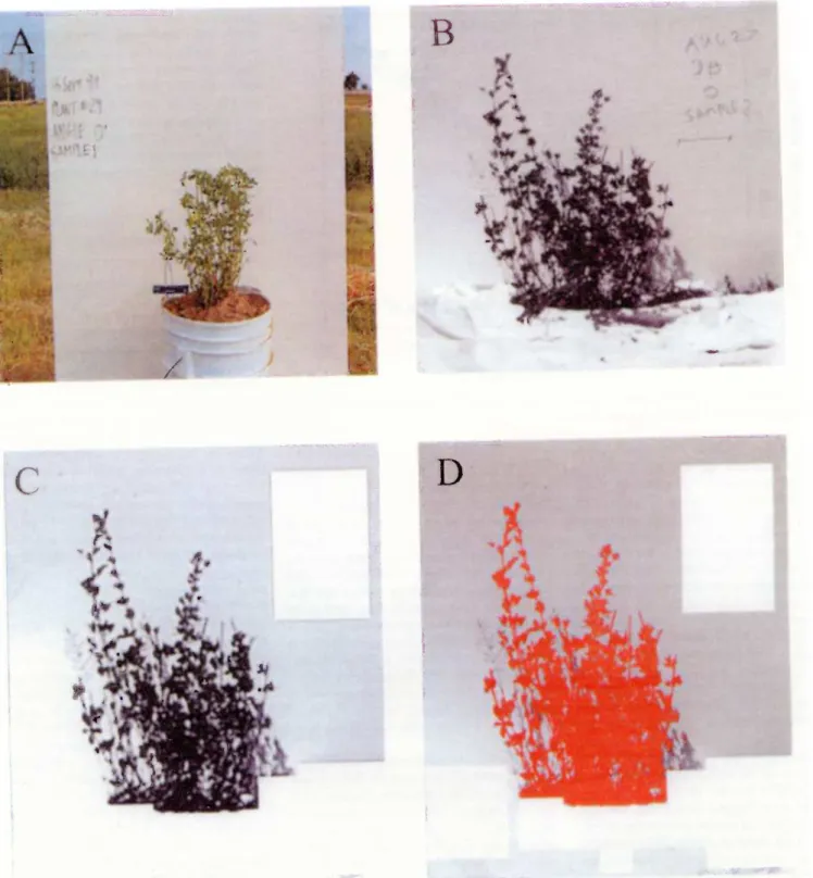
To separate the plant from the back- ground, a sheet of white, dry-erase board was placed behind, but not touching, the plant (Fig. 1A). Plant identification, date, sample number, and photo angle were recorded on the dry-erase board. A ruler attached to a wire was placed to the side of the plant on a plane bisecting the midpoint of the plant. Each ruler was held in place by inserting the attached wire into the soil.
A second ruler was placed perpendicular to the first, also on a plane bisecting the plant's midpoint. These rulers served to calibrate the image and to establish 0 and 90° reference angles. To improve calibra- tion accuracy, the rulers were trimmed to a total length of 10 cm, eliminating the need to see the marks on the ruler.
A digital camera (Kodak® DC260) was used to photograph the plants. Two pho- tographs were taken at each sampling stage (sample 0-k) with the first 2 taken prior to defoliation (sample 0). The first photograph of each pair was taken at the midpoint of the plant height and width from a direction minimizing shadows. The second was taken at 90°, on a horizontal plane, from the first. The white backdrop
was also rotated at each step.
Plants were hand-defoliated in 5 steps.
Approximately 20% of the total plant weight was removed and collected as a sample during each step. As each sample was collected, the sample number was recorded on the backdrop and the plant re- photographed. Succeeding photos were taken from as close to the same position as possible. Samples collected at each step
were bagged and labeled separately.
During the last defoliation step, all
remaining above ground tissue was removed. Each sample was dried at 60° C for 24 hours prior to being weighed to the nearest 0.5 g. The weight of each defolia- tion was recorded and then summed to determine total weight of the plant.
Image Analysis
Jandel's SigmaScan Pro® 3.0 was used to analyze the digital images. Any image analysis software could be used provided it has something approximating the fol- lowing capabilities: image cropping, cali-
bration of scale, color/black and white/contrast transforms, intensity selec- tion procedures, and some form of data reporting program. These are used to pre- pare the image of the plant for areal mea- surement. Image cropping helps isolate the target image from incidental objects. This will become important as the technique evolves for use in the field. Once the image is adequately prepared, the program counts pixels of various values that cone- spond to the image. These pixels are then transformed to area based on the measure- ment of a known distance on the image, in this case the 10-cm ruler, to the number of pixels contained in the length of the image of the ruler. Color/black and white/contrast transforms and intensity selection proce- dures enhance isolation and measurement of the target image (Fig. 1B, C, and D). In our method, the color image was trans- formed to black and white (grayscale) due to the program we used being better able to delineate the image in black and white.
Once the measurements are made, such that a calculation of area for each image is available, the data can be copied into a spreadsheet for further analysis.
Sample weights and photographic areas were converted to percent weight remain- ing and percent area remaining, respec- tively. We used a mean calculated from the percent remaining areas for angles 0°
and 90° to address the 3 dimensional aspect in a 2 dimensional form. Forty plants were used to develop a statistical model and 10 plants to test the model. To test for repeatability of the image analysis, we calculated the area for 1 plant image 10 times. To test sampling precision, we calculated the mean deviation from the desired 20% defoliation sample size and standard deviation of this mean for the samples taken from the 40 plants used to build the model.
Model Building
A statistical model was constructed to provide estimates of individual plant uti- lization, specifically for this particular
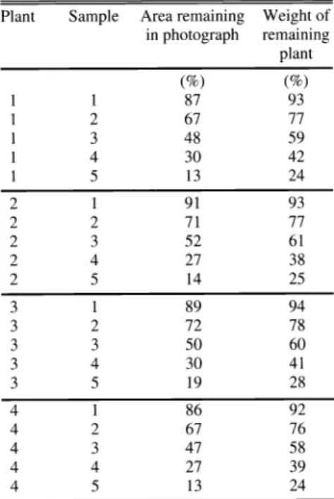
Table 1. Example data used to demonstrate statistical methods.
Plant Sample Area remaining Weight of in photograph remaining
plant
(%) (%)
1 1 87
3 1
1
1
2 2
3 2
2
3 1
2 3
4
3 5
4 1
4 2
4
4 4
4 5 13
variety of alfalfa (Malone) at this particu- lar stage of growth. The random coeffi- cient (RC) model was used and can be written as [yij = (30 + si + (1 + di)xij +
i=1... n and j=1, k] where yij is the percentage of the ith plant remaining after the jth sample is removed, is the remain- ing area covered in the photograph of the ith plant after the jth sample is removed,
(30 is the y-intercept, 1i is the slope, and
Si, di, and are random effects in the model associated with the random devia- tion of the ith plant's intercept from the intercept (3p, the random deviation of the
ith plant's slope from the slope f 31, and ran- dom error, respectively (Graybill 1976).
The first step in building the RC model is to estimate a simple linear regression (SLR) equation for each plant. Each SLR equation describes the straight-line rela- tionship between the percentage of remaining plant (y) and the percentage of remaining area covered in the photograph (x) for a single plant. In general notation, let bpi and b 1 i denote the estimated y- intercept and slope for the ith plant (i = 1,..., n). Computations were performed using fifteen significant digits and rounded to one for illustration purposes. The esti- mated SLR equation for the ith plant is
= b0i + blixi.
A small subset of the data set (n = 4, k = 5) is given in Table 1 to use in illustrations of the statistical computations. The esti- mated SLR equations and associated sums of squared residuals for each of the 4 plants in Table 1 are reported in Table 2.
JOURNAL OF RANGE MANAGEMENT 56(2) March 2003 141
Table 2. Estimated Simple Linear Regression (SLR) equations and Sum of Squared Residuals relating the percentage of remain- ing plant (y) to the percentage of remaining area covered in the photograph (x) for each plant in Table 1.
Plant SLR Equation Sum of Squared Residuals
1 y =13.25 + 0.9337x 6.9594 2 y =13.77 + 0.8829x 4.7088 3 y=12.15+0.9241x 7.5185 4 y =13.24 + 0.9283x 4.9426
The y-intercept and slope of the RC equation are estimated by computing the sample averages of the estimated individ- ual plant y-intercepts and slopes, respec- tively. The estimators for the y-intercept and slope can be written as
and
_ l n
_ -b0i
n t=1
1 -
(1)
(2)
respectively. For our example,
4
fl0 = -- b01=(13.2+13.8+12.1+ 13.2)/4 =13.1 41=1
and /1 =
- l b11= (0.93+0.88+0.92+0.93)14 = 0.92
4=1
Thus, the estimated e nation for the RC model is y ij = (30 + 1 x = 13.1+0.92x for this example.
The estimated mean of y at a given value of x (say x*) is
(Y1XX*)fl0+fllx* (3)
For the example, an estimate of the per- centage of a plant remaining that was observed to have, say, 80% of the area remaining in a photograph of the plant after it was browsed by an animal, is y given x = 80 or (91 x = 80) = 130 + (31(80)
=13.1 + 0.92x = 86.5.
Results and Discussion
Theoretically, the limit for detection of biomass removal should correspond to the area of the photo covered by a pixel given that the tissue removed is on a plane visi- ble to the camera, i.e., not hidden by inter- vening tissue. This plane of visibility is probably the most important source of variation in the individual plant models.
Photographing plants from perpendicular directions and taking the mean area of the 2 images helped to reduce variation incor- porated into the model by the 3-dimen- sional shape being reduced to 2 dimen- sions during analysis. Estimates of the remaining percentages of plant weights were accurate to +/-21% using the 0°
angle photographs and to +1-17% using the 90° angle photographs, but were accu- rate to +/- 8.5% using the mean of the 0°
and 90° angle photographs. The mean area for the repeated images was 676 cm2 (SD
= 21.61, CV = 3.19, n = 10). The basic premise, that a pair of photographs taken at perpendicular angles can adequately model the 3-dimensional plant, seems to hold up well.
Problems encountered were the inabili- ty to distinguish plant tissue from back- ground clutter, poor image quality, and increasing area with decreasing biomass.
The backdrop solved the background clut- ter problem. Using a digital camera and image manipulating software allows the operator to manipulate image factors and does much to solve image quality prob- lems. The area-biomass problem is typi- cally the result of allowing the background screen to contact the plant or photograph- ing the plants under windy conditions thereby changing the apparent area
between photographs. These 2 factors are the main contributors to the plane of visi-
bility problem mentioned above. To ensure the repeat positioning of the cam- era for sequential shots, one could use 2 tripods placed at right angles to the plant and simply move the camera between the tripods. The use of quick release heads on the tripods would facilitate this approach.
With SigmaScan Pro® 3.0, the set thresh- old routine is a potential source of subjec- tivity. Carefully setting the threshold val- ues in the first image so that plant tissue is
maximized and extraneous material is minimized and then holding this value constant throughout the series of images will minimize the subjectivity inherent in this step. Figure 1D shows an example of a threshold setting where plant tissue is highlighted, but shadows and grass stems are not.
There are additional considerations if film is used. In a previous trial, we used Kodachrome, 64 slide film. Upon return of the processed slides, they were digitized with a Nikon Coolscan® slide digitizer.
This gave us good control over the image quality with respect to setting up the image for further analysis. Prints could possibly be used with a flatbed scanner, but the superior resolution, for a given
film speed, of slides vs. prints may argue against the use of print film. This differ- ence in resolution is due to the inherent loss of information that occurs when an image is transferred to a different medium, i.e., film negative to paper. It is possible that this loss of resolution would be too small to have an effect on this technique.
A fast film (ISO of 200 or more) used with flash would enable working during periods of light to moderate winds. The use of a flash should help reduce problems created by shadows. Depth of field should be maximized so that the entire image of the plant is as sharp as possible.
Time investments in this technique are somewhat longer than with previous meth- ods listed in Table 3, but the improved
Table 3. Comparison of methods for estimating utilization.
Method Time Accuracy
(days)a (%) Digital Photographic 4 ± 8.5
Ocular by Plotb 2 + 19
Ocular by Plantb + 2
Leaf Lengthb + 16
Plant Countb + 26
Height/Weight Ratio + 10-25 aTime
includes model building and training.
bPechanec and Pickford (1937) (these values are means).
Clark (1945).
results offset the increased time invested.
Collecting samples and photographing alfalfa plants took an average of 20 min- utes/plant. A large part of the post-sam- pling time spent depends on the camera used. Digital cameras provide usable images immediately. Turn-around time for development of film is dependent on whether the film is sent to a lab or devel- oped in house. Once slides, or digitized images, are available, the process takes 3
to 5 minutes per image to calculate the variables of interest. This data is then tran- scribed to spreadsheet form and appropri- ate statistical analyses completed. Training of inexperienced individuals could proba- bly be done in 2 sessions of roughly 4 hours each, an hour each for photography, digitizing, image analysis, and data collec- tion plus some time to practice the tech- nique. Once simple linear regression equa- tions are computed for each plant, con- struction of the random coefficient model is relatively easy.
Statistical analysis of this data set using simple linear regression across all plants would seem to be an intuitive approach.
An important assumption associated with simple linear regression (SLR) is that the
142 JOURNAL OF RANGE MANAGEMENT 56(2) March 2003
Fig. 1. A. Apparatus for separating plant from background. B. Image set in black and white. C. Cleaned image. D. Image ready for measuring.
random variable (y) at each value of x is independent of the random variable y at any other value of x. In the present work, sequential samples were taken from each plant resulting in measures of biomass (y) at various values of area (x) that are not independent of each other. The RC model addresses the problem of a lack of inde- pendence by using the line produced for
each plant by simple linear regression as the attribute of interest. From a statistical perspective, this approach is preferred because the estimates are more precise and because the sources of variability can be partitioned and examined to improve
future models.
The RC model fit to the data from 40 of the alfalfa plants resulted in the equation
[Yip = 9.06 + 0.976x]. Figure 2 shows the estimated and observed percentages of plant remaining for sample points from 10 plants not used in constructing the model.
There is an increased sensitivity at lower levels of defoliation. The greater sensitivi- ty is advantageous due to desired utiliza- tion levels, which usually requires leaving more than 50% of the plant.
JOURNAL OF RANGE MANAGEMENT 56(2) March 2003
143
0 20 40 60 60 100
Observed Ptent Weight (g)
Fig. 2. Estimated vs. observed plant weight remaining with 95% confidence intervals for 10 alfalfa plants with 4 samples from each plant.
The optimal sample allocation between number of plants and number of samples per plant is dependent on plant morpholo- gy. However, because of statistical
assumptions of normality, we recommend no fewer than 30 plants. The optimal num- ber of measures per plant is dependent on the researcher's experience with the sam- ple/photographic methodology. However, for purposes of fitting the RC model, a minimum of 4 measurements per plant including the whole plant measurement is required. The researcher must conscien- tiously attempt to select samples at the same x-values for each plant to meet sta- tistical assumptions of the model. For our samples, the mean deviation from the ideal 20% intervals between areas of consecu- tive samples within a plant for the 40 plants used in building the model was
12.5% (SD = 6.2, n = 160).
One of the biggest drawbacks with cur- rent methods of forage and browse utiliza- tion is the level of subjectivity required.
Ocular estimates rely on the experience of the observer and may be subject to indi- vidual bias, particularly if the observer is not well trained or fails to periodically check his observations against a standard (Bement and Klipple 1959). Height/weight methods generally perform well, but are dependent on plants used to develop the model being similar in morphology to the plants being estimated (Clark 1945). The technique described in this paper incorpo- rates aspects of several methods. It is simi- lar to ocular-estimate-by-plant and height/weight methods in that individual
plants are used as the basic units and a
weight/area relationship is developed (Lommasson and Jenson 1938, Cook and Stubbendieck 1986). The digital-photo- graphic method minimizes subjectivity through the use of photographs. Repeated measurements of an image gave a coeffi- cient of variation of 3.19%. Due to varia- tion in plant morphology across species, seasons, or sites, a model may need to be developed for each application (Caird 1945, Clark 1945). Once a model for a given plant is developed, it should be use- ful indefinitely. We do not know at the present time what the limits on usefulness are for a given model, say alfalfa, when applied to a plant with a different mor- phology.
Collection of plant samples and their related photographs can be done fairly rapidly in the field and subsequent model- ing and analysis completed in the labora- tory. Additionally, photographs from sites to be analyzed for forage utilization can be taken and analyzed at a time convenient to the individual doing the assessment. A series of forage conditions could be pho- tographed at intervals throughout the sea- son and an analysis of season-long changes could be carried out. This tech- nique will be difficult to use on large shrubs or trees due to the limitations of harvesting the entire plant for modeling.
Estimates of weight/unit area may allow the use of this method for large shrubs or trees although indirect methods are proba- bly of more value (Bonham 1989). Also, this method has not yet been tested on
grasses or woody plants. Any situation where individual plants can be delineated in the field of view will probably work.
Situations where plants are in close prox- imity, such as turf, may be problematic.
As software of this type develops, the use of variation in color will likely improve the ability to differentiate specific targets and thereby improve the utility of digital- photographic methods such as the one pre-
sented here.
Conclusions
The digital-photographic method described herein accurately estimated the weight of individual alfalfa plants at sequential defoliation episodes to within ± 8.5%. The weight values were calculated from paired perpendicular photographs taken of each plant at each level (0, 20, 40, 60, 80, and 100%) of defoliation. Time needed to complete the model building varied from 22 to 32 hours total time depending on familiarity with techniques.
Once an appropriate model is developed for a plant species, objective estimates of plant material present can be readily cal- culated based on photographs of the plant.
Before and after photographs will give estimates of plant biomass removed, or remaining, if photographs are obtained in short enough temporal intervals that plant growth or leaf abscission does not become a confounding factor. Within this context, plant phenology should not affect esti- mates. The use of a digital-photographic method for estimating plant biomass lost to herbivores has applications in agricul- ture, ecology, and other fields. As image analysis technology improves, the applica- bility and accuracy of techniques such as this will improve. One aspect in particular need of improvement is the ability to sepa- rate target plants or groups of plants from background objects. For most shrubs and forbs in arid and semiarid environments that have a random or regular distribution, the problem associated with plant separa- tion should be minimal. In all cases, the use of blocking objects, such as the back- ing board used here, will be needed to sep- arate the plant from its background. The use of readily available computer technol- ogy and photographic equipment will decrease the subjectivity and increase the accuracy of field measurements of plant geometry and associated losses due to her- bivory and/or other factors.
144 JOURNAL OF RANGE MANAGEMENT 56(2) March 2003
Literature Cited
Bement, R.E. and G.E. Klipple.1959. A pas- ture comparison method of estimating uti- lization of range herbage on the central Great Plains. J. Range Manage. 12:296-298.
Bonham, C.D.1989. Measurements for terres- trial vegetation. John Wiley & Sons, New York, N.Y.
Caird, R.W. 1945. Influence of site and graz- ing intensity on yields of grass forage in the Texas Panhandle. J. Forest. 43:45-49.
Clark, I. 1945. Variability in height of forage grasses in central Utah. J. Forest.
43:273-283.
Cook, C.W. and J. Stubbendieck. 1986.
Range research: basic problems and tech- niques. Soc. Range Manage., Denver, Colo.
Estell, R.E., E.L. Fredrickson, D.M.
Anderson, K.M. Havstad, and M.D.
Remmenga. 1998. Relationship of tarbush leaf surface terpene profile with livestock herbivory. J. Chem. Ecol. 24:1-12.
Graybill, Franklin A. 1976. Theory and appli- cation of the linear model. Duxbury Press, North Scituate, Mass.
Holechek, J.L., R.D. Pieper, and C.H.
Herbel. 1989. Range management: princi- ples and practice. Prentice Hall, Engelwood Cliffs, N.J.
Lommasson, T. and C. Jensen. 1938. Grass volume tables for determining range utiliza- tion. Sci. 87:444.
Pechanec, J.F. and G.D. Pickford. 1937. A comparison of some methods used in deter- mining percentage utilization of range grass- es. J. Agr. Res. 54:753-765.
Society for Range Management. 1974. A glossary of terms used in range management,
2nd Edition. Soc. Range Manage., Denver, Colo.
JOURNAL OF RANGE MANAGEMENT 56(2) March 2003 145