Munich Personal RePEc Archive
Size effect in transitional dynamics of the
banking network
Garcia, Alfredo Daniel and Szybisz, Martin Andres
Instituto de Investigaciones Económicas, Facultad de Ciencias
Económicas, Universidad de Buenos Aires
15 June 2017
Online at
https://mpra.ub.uni-muenchen.de/80195/
Size effect in transitional dynamics of the banking network
Alfredo García y Martín Szybisz (1)
We consider a developed economy banking system, that, when surpass certain size, may
destabilize and even enter in chaos. Taking Deposits (𝐷𝑡), Reserves (𝑅𝑡), Loans (𝐿𝑡), the ratio
of (𝑅𝑡) to (𝐷𝑡) and a parameter 𝛾 that weights endogenously the system memory, we analyse
stability and the possibility of chaos. Using data for the U.S. between 1960 and 2012 we
found that a maximum instability state is verified in 2008 when the crisis hits the U.S.
banking system core carrying to a public bailout. A larger system does not necessarily lead to
robustness but can expand to greater fragility. A proposed banking system stability indicator
is also analysed.
Key Words: Banking System, Financial Crises, Instability, Systemic Risk, Chaos
JEL: G01 - Financial Crises
“Credit driven boom bust cycles are temporally asymmetrical.
The build up is slow and long, the collapse quick and sudden.
In Hemingway’s The Sun Also Rises, one of the protagonists Asks his friend: “How did you go bankrupt?” “Two ways”, went the answer, “gradually, then suddenly.” (Leijonhufvud, 2013)
1. Introduction
(1 )University of Buenos Aires, Faculty of Economic Science, Institute of Economic Research, UBACyT (UBA 2013-2016) and
Systemic banking crises are rare events that strike in the middle of credit booms and are
followed by long and deep recessions (Boissay, Collard and Smets 2013). Bank crises
produce, among other consequences, payment chain disruptions and uncertainty on asset
values and on debt re-payment capabilities.
Part of the economic literature associates financial (and aggregate economy) instability to
fractional reserves banking systems (Cochrane 2012). By contrast, those advocating the
benefits of bank credit point to the emergence of credit bubbles that are not sustainable over
time as a source of instability (Schularick Moritz, Taylor 2009).
Traditional financial literatures see the origin of systemic banking crises as a classic situation
of depositors panic or a mismatch in the interbanking flow of funds. Others (Diamond - Rajan
2005) pointed out to a rapid transmission of liquidity shortages as a cause of contagion that
eventually turns into widespread insolvency.
Great efforts have been done in studying the sources of instability and fragility of the
economic structure. An aspect of fragility we consider here is the growth of income inequality
as a source of insolvency. Authors like Michael Kumhof and Romain Rancière (2010)
employed a theoretical framework to explore the link between revenue enhancements enjoyed
by high-income families; poor and middle classes increased indebtedness and financial
system's vulnerability.
The bank system grows by accumulation of deposits of top income households and loans to
maintain lifestyles of middle and low income sectors. The flip of a complex dynamical system
from a state of steady growth to a highly unstable one, “may be initiated by some obvious
external event, such as a war, but is more usually triggered by a seemingly minor
happenstance or even an unsubstantial rumour” (May, Levin and Sugihara 2008:893). A
minor increase in the bad debt ratio in some banks portfolios in a highly interconnected
system with fast feedback mechanisms within it and slight changes in their loan policy, may
become suddenly an explosive situation and afterwards “will exhibit some form of hysteresis,
such that recovery is much slower than the collapse. In extreme cases, the changes may be
irreversible” (May, Levin and Sugihara 2008:893). The impact of an unexpected increase in mortgage defaults, next to a drop in property values, may be taken as a minor change in the
One way of representing systems is with a network. In this paper we adopt this view of the
banking structure as a system. This implies that it possess at least nodes (banks, not
necessarily all of equal size) and interconnections of different kinds. The topology of the
banking network has been studied in detail in reference to the number of connections, the
degree of interconnectedness, and of assortativity (Loepfe, et all and its cites, 2013). In his
work the authors affirm that relevant properties of real world banking systems includes high
clustering; size heterogeneity and sensibility to contagion even with low density connections.
The authors also point out that “the transition from safe to risky regimes can be very sharp”
and that the range for this “is situated at low link densities and high values of modularity and
size heterogeneity. Crucially all real world examples found in the literature show precisely
these characteristics”.
We will adopt those results and analyze the stability of this kind of networks. Of the many
topological characteristics of the banking network we select to investigate the relationship
between an increasing size of the network and its effect on stability. In this work we take size
as the quantity of deposits that the banking system operate. This definition allows
comparability and consistency in different moments of time and place2.
A larger banking system has been seen, before the 2007 crisis in the U.S, as a beneficial
element, even by international financial institutions as the IMF. Bank concentration, was a
sign of strength (Beck, Demirgüç-Levine 2006). In marked contrast, May, Levin, & Sugihara
(2008) presented an argument that the combination of large size and high inter-connectivity
can be, as in ecological systems, a source of instability.
As the UK Financial Services Authority point out in the Turner Review (Turner 2009) “the
shift to an increasingly securitised form of credit intermediation and the increased complexity
of securitised credit relied upon market practices which, while rational from the point of view
of individual participants, increased the extent to which procyclicality was hard-wired into
the system”. The systemic risk associated to an increase in the size of the system by keeping
unchanged the “hard-wired” interconnection is the subject of our work.
2Alternatively; “size of the banking system” as “quantity of bank entities” have some drawbacks. It may be
An unexplored approach, intended herein, is to analyze the effects of the banking network
size change 3 and explore some critical events (for example, the amount of US banking credit
trend break in 2008 (Figure 2); where the system suddenly change from a long stable period
of growth to a widespread recession).
Very simple nonlinear systems can have very complex dynamics (Aulbach & Kieninger
2001). Small changes in critical variables produce unexpected and unpredictable results
modifying abruptly the development of the system (Fichter 1998). Apparently predictable, the
system starts to behave in an unexpected way in a short period of time and stabilizes
afterwards, but in a different trajectory.
Vitali, Glattfelder and Battiston (2011) shown that models with systemic-risk propensity are
characterized by high connection density (interconnectivity). Instead of strength,
concentration may increases fragility.
2. Stylized Dynamics
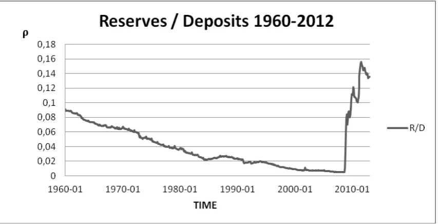
Over a long period of time (50 years) the US banking sector increased deposits and loans
successfully with a declining reserve ratio 𝜌 (see Figure 1). This growth was not seen as a
problem neither by the authorities nor by the markets, until, unexpectedly, severe
complications emerged.
3 Stability defined as absence of excessive fluctuations of the variables and convergence when small shocks
occurs (see for instance Heijdra, B. J., 2002;Romer, 2006; Shone ,2002).
Figure 1
Source: Board of Governors of the Federal Reserve System, "Bank credit, all commercial
banks".
Banks monitor the ratios between deposits, loans and non-performing loans daily. As far as
the net present value of their portfolios remained within the expected level of profitability; in
an environment of declining interest rates and low inflation, the expansion can last a long
period of time (Figure 2). Loans supply feeds positively the economic growth while the
financial system grows in its size.
Figure 2
[image:6.595.71.508.526.737.2]But future expected values may or may not be achieved. If present value of the portfolio falls
due to an increase in non-performing debt, one or more banks may try to reduce loan
portfolios exposure and increase reserves. If the system is large and highly interconnected,
such individual behavior can spread quickly.
A sustained upward trend of deposits 𝐷𝑡 over time can be postulated (necessary condition to
increase the size of the system) even with constant money circulation velocity, no money
quantity increase and the absence of endogenous money creation. The source of this growth
may come, instead, from the accumulation of financial surpluses by economic agents (for
simplicity we call them rentiers) that, having a steady flow of income that they cannot
consume; turn this resources to various financial instruments. Such agents are, for example,
Sovereign Wealth Funds and Pension Funds (Garcia & Nicolini 2012 and they references).
Rentiers decide whether fully or partially placed such surplus in the banking system, changing
the volume of deposits in the system. The variation of deposits and therefore the trajectory of
𝐷𝑡 is defined by the sum of the individual decisions of each rentier. These surpluses received by banks are in turn placed as loans 𝐿𝑡 for those agents who spend above their income, that is
to the net debtors of the system (an effect of this asymmetry can be found in the existence of a
rate return on financial income which is secularly above the growth rate of the economy
(Piketty 2014, Garcia & Nicolini 2012 and they references)).
The behavior of rentiers in deciding whether or not to keep their surpluses in the banking
system can be considered as a random walk because of the autonomy of decision of each
rentier. However it is possible to think that in certain situations groups may form that act
coordinately, increasing deposits or making withdrawals. This approach postulate that they
may form coalitions (clusters); each replicating certain strategy, supporting long periods when
influx of deposits dominated and other critical periods where the decision to withdraw
dominates. Such cases of “behavior copy” (herd behavior) have been studied in models of
financial markets (Eguiluz, V. M., & Zimmermann, M. G. 2000). They can be used to analyse
situations when portfolio decisions are concentrated in a reduced group of investment fund
administrators and banks strategy leads to create products to recover liquidity like
securitization schemes of less liquid assets such as costumer loans or mortgages.
A tendency to the growth of the banking system may be seen as a more than proportional
increases in deposits relative to GDP. Within this kind of scenarios, the connection of
proposed by Cont, and Bouchaud (2000) and Eguiluz and Zimmermann, M. G. (2000), for an
asset market. Decisions to buy, sell or stay inactive are associated with coalitions of actors
(clusters) that follow the same strategies. In Cont, and Bouchaud (2000) the size distribution
of these coalitions are made dependent on a parameter that arises from the probability that two
agents are linked together. A higher probability of connection increases the size of the clusters
and reduce the number of clusters in proportion to the size of the system.
With this background in view, we may assume that, in a long period of expansion, a larger
number of rentiers surpluses is deposited in banks accounts, forming clusters of agents with
the same opinion over business conditions. A concrete dynamic develop as follows. The
growth of deposits lead to an increase of long term credits like mortgages. The increase in
demand lead to an increase in the value of assets, such as real estates; what in turn elevate the
amount of the new credits and exposes the system to a greater risk of bad loans. Once big
clusters have been formed a critical situation could lead to massive withholdings of funds and
then a sharp decrease of deposits take place. The fundamental stylized fact for the model to
work is that of deposits growing over time.
In due course, deposits become loans, and all the bank system remains in a steady growth
path. Our work analyses what happens when the growth of deposits leads to a growth of
loans that cannot be sustained indefinitely; eventually stops abruptly and reversed it trend
going (possibly and temporarily) into chaos.
3. The model
Let’s consider the aggregate banking sector of a developed economy and the following
variables and parameters.
𝐷𝑡= Deposits of period 𝑡
𝑅𝑡= Reserves of period 𝑡
𝐿𝑡= Loans of period 𝑡
𝜌𝑡= Reserve ratio (reserve holdings of banks to demand deposit liabilities) in period 𝑡
𝑅𝑡 = 𝜌𝑡𝐷𝑡 (1)
𝐿𝑡 = (1 − 𝜌𝑡)𝐷𝑡 (2)
Bank decisions on Reserves for each period are related to the Reserves/ Deposits ratio of the
previous period and are condensed in equation (3). Usually, the more Loans the larger the
Reserves needed(Bagehot, 2004).
𝜌𝑡+1= 𝑓(𝑅𝑡, 𝐿𝑡) (3)
Therefore,
𝜌𝑡+1= 𝛾𝑅𝑡𝐿𝑡 (4)
Equation (4) has some properties that a function, that relates the coefficient of reserves to
previous reserves and loans, is expected to have. The multiplicative form indicates that both;
reserves and loans must not be zero as a necessary condition to the existence of the
coefficient. In other words reserves and loans are not separable. The derivative of 𝜌𝑡+1
respect to reserves and loans is positive and related to the other component. For instance,
if 𝐿𝑡 grows 𝜌𝑡+1 is incremented by the proportion 𝛾 of 𝑅𝑡. There is a unit-elasticity of
𝐿𝑡 and 𝑅𝑡 respect to 𝜌𝑡+1; witch is one way to review consistency; indicating that when reserves or loans changes, 𝜌𝑡+1 varies proportionally. When 𝐷𝑡varies the function does not
define if 𝜌𝑡+1 grows or get smaller, what is consistent with the empirical data of graph 2.
The use of an aggregate and unique 𝛾 with an equal decision period for all agents depends on
the assumption that the sector has fast and flexible interconnections and efficient transmission
mechanisms.
Taking equation (1) one period forward and replacing (4) into it;
𝑅𝑡+1 = 𝛾𝑅𝑡𝐿𝑡 𝐷𝑡+1 (5)
𝑅𝑡+1= 𝛾𝑅𝑡(1 − 𝜌𝑡)𝐷𝑡𝐷𝑡+1 (6)
And by equation (1) together with (6)
𝑅𝑡+1= 𝛾𝑅𝑡𝐷𝑡+1(𝐷𝑡− 𝑅𝑡) (7)
Logistical functions with one lagged period are used in Macroeconomics to account for
nonlinearities and at the same time are reasonably simple from the mathematical point of view
(Sordi 1996).
Following Shone (2002) we consider the equilibrium for this type of model. For 𝑡0, the
solution value is 𝑥(𝑡0) = 𝑥∗. The fixed point 𝑥∗ is called “steady state” or “equilibrium
point”.
A fixed point is asymptotically stable if any trajectory, started near it, approaches it as 𝑡 → ∞.
We use the concept of equilibrium or fixed point to denote the position where the variables do
not change (the first derivative with respect to 𝑡 is zero) (Shone 2002).
The fixed point in (7) is given by:
𝑅∗= 𝛾𝑅∗𝐷∗(𝐷∗− 𝑅∗) (8)
Where 𝑋∗ denote the value of the variable 𝑋 at the fixed point.
𝑅∗=𝛾𝐷∗2− 1
𝛾𝐷∗ (9)
For a positive level of reserves it must be that:
𝛾𝐷∗2> 1 (10)
From the other side the maximum level of Reserves is given by taking the first derivate of
𝜕(𝑅𝑡+1)
𝜕𝑅𝑡 = 𝛾𝐷𝑡𝐷𝑡+1− 2 𝛾𝐷𝑡+1𝑅𝑡= 0 (11)
The maximum level in t+1 would be 𝑓 (𝐷𝑡
2). Replacing this result in (7)
𝑅𝑡+1 = 𝛾𝐷2 𝐷𝑡 𝑡+1(𝐷𝑡−𝐷2 ) =𝑡 𝛾𝐷𝑡 2𝐷
𝑡+1
4 (12)
The maximum amount of Reserves could not be greater than the total Deposits;
𝛾𝐷𝑡2𝐷𝑡+1
4 ≤ 𝐷𝑡+1 → 𝛾𝐷𝑡2≤ 4 (13)
This means that
1 < 𝛾𝐷𝑡2≤ 4 (14)
It is easy to recast equation 4 (7) in the usual form of the logistic equation
𝜌𝑡+1 = 𝛾𝐷𝑡2(𝜌𝑡− 𝜌𝑡2) (15)
Considering (7) and (14) we find a cycle which includes the possibility of chaos for any value
for𝛾𝐷𝑡2 above 3.57. Let us call this parameter “stability coefficient”, since this number is a
parameter of the logistic equation (15) whose characteristics are well known and possess all
the information necessary to know the dynamic stability of the relation between deposits,
loans and reserves5. It is worth to mention that once the stability coefficient is calculated for
4 As pointed out by Professor Kawamura, the limit value for chaos (2.57) indicate by Shone (2002) seems to be
incorrect. Indeed, equation (7) of our model equation can be written in the general form of the logistic equation that has a well-known limiting value of 3.57 as Shone itself point out writing in general about the logistic equation.
5 This value was originally found by Benhabib and Day (1981) in a consumer choice model that produces chaos
each period it remain fixed for the projections that can be made using it. Giving the value of
the stability coefficient, the reserve percentages may be calculated iteratively for some
temporal horizon. Our empirical review for data of commercial banks of the US Federal
Reserve Bank system6 (see below) showed that the nearest point to the limit value of 3.57 was
in September 2008 (reaching 2,92), from 2,19 in August going to 1,95 in October of that year.
The relevance of 𝐷𝑡2 is linked to the importance of the system size (see below). Briefly, 𝛾𝐷𝑡2 7
shows how the memory of the system represented by 𝛾 reacts to its total size 𝐷𝑡. If the agent’s
decisions are based on their present common experience (past experience memory), once the
system grows, it may enter into instable regimes and even chaos. In practical terms these
means that the dynamics of decisions on reserves of the past is no longer a valid guide for the
future.
Decisions on bank Reserves level, using the 𝛾 parameter, could provide useful information
about certain characteristics of the system. If 𝛾 is unique and the decision period the same for
all agents, the system is highly interconnected and concentrated (at least, at the decision
making level). Both characteristics elevate the probability towards a regime that have the
potential to be chaotic.
In this way, the γ parameter may not only represents the memory of the system, but also interconnectivity and concentration, characteristics that may be present in the banking system
taking in account our discussion in section 2.
4. Empirical Evidence
First, we will evaluate whether the proposed relation in the previous section between 𝑅𝑡
and 𝑅𝑡+1 approximate the empirical data of the Federal Reserve for aggregate data of
6By that time several businesses and institutional depositors withdrew money from their accounts in order to drop their balances below the $100,000 insured by the Federal Deposit Insurance Corporation (FDIC) – an event known in banking circles as a "silent run." The fourth bank of the Federal Reserve System, the Wachovia , lost a total of $5 billion in deposits in one day—about one percent of the bank's total deposits- and was pressured by the federal authorities to put itself up for sale over the weekend (Charlotte Observer 2008).
commercial banks of the US. The period 𝑡 is a month in our calculations for all variables
[image:13.595.74.513.187.387.2]and parameters; we use monthly data at the beginning of it.
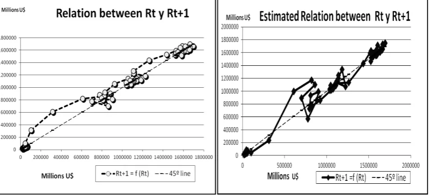
Figures 3 and 4
Reserves (in millions of dollars)
Figure 3, Source: Board of Governors of the Federal Reserve System 1960-2012 adjusted by
inflation (Federal Reserve of Saint Louis). Figure 4: based on our model using the relations of
𝛾 and 𝑅𝑡, 𝐿𝑡 given in equation 4 to calculate 𝑅𝑡+1 respect to 𝑅𝑡.
Figure 3 shows the relationship between 𝑅𝑡 and 𝑅𝑡+1 observed for the Federal Reserve
System for the period between 1960 and 2012. The points above the 45° line indicate that the
system accumulates reserves. From 1960 until August 2008, Reserves were kept in the range
from 20 to 45 billion dollars and are represented by the small cluster shown on the origin. The
first significant point is August 2008 when Reserves jump to almost 103 billion. From then on
an unstable loop emerges and remains for one year until Reserves stabilize near the 110
billion dollar mark. The system keeps accumulating Reserves with more fluctuations in the
range of 160/170 billion until year 2012.
Figure 4 shows the result of our estimation using 𝛾 to calculate 𝑅𝑡+1 respect to the 𝑅𝑡 when
instability and subsequent fluctuations emerged in 2008. Since the system calculates an
expected reserve ratio based on the levels of reserves and deposits of the previous period,
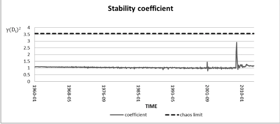
Next, we calculate the stability of the 𝛾𝐷𝑡2 value. Figure 5 shows the results of our model. It
is worth to mention that the period for which the stability coefficient may be useful would be
normally very short. The stability coefficient is an initial condition and the logistic equation is
very sensible to small changes in the initial conditions9. The value for the coefficient obtained
may generally be useful in a high frequency environment; that is time slot of minutes and
hours. The longer the time slot the less useful the coefficient.
Given that Macroeconomic data does not appear for very short time periods and in the aim of
[image:14.595.70.524.258.460.2]covering the bigger period possible we have taken monthly data to build our empirical review.
Figure 5
Source: Own calculation, based on statistical data of the Board of Governors of the
Federal Reserve System 1960-2012 adjusted by inflation (Federal Reserve of Saint Louis).
We estimate 𝛾 using the relation of equation 4 taking available data of 𝜌𝑡+1, 𝑅𝑡 and 𝐿𝑡.
During 2008 the system registered the most important instability close to chaos for the
considered period. Some instability respect to registered values also emerged in 2001.
9 As Lorenz point out: “Chaos: When the present determines the future, but the approximate present does not
The system does not go through an adaptive transition phase before the instabilities, which is
a hint that a chaotic situation could be considered in the theoretical analysis of the U.S.
financial crisis of 2007 – 2008. The agents within the system, probably in grasp of some
variables of his environment; may had had difficulties in processing the small changes in
information that leads to the crisis.
Another relevant fact is that, despite that the instable situation is quickly surpassed the system
appears to behave relatively more unstable and oscillatory than before, as it is shown in figure
5.
Therefore, even with a deterministic model (not stochastic), infinitesimal changes that
accumulate (see Figure 1) in a growing system (see Figure 2) may cause a sudden and
significant change leading to an instable (near chaotic) situation (see Figure 4 and 5); since it
is impossible to know (like in any other chaotic system10) with sufficient precision which or
how to modify previous decisions practice.
5. Is it a real state of chaos?
From the monthly data, although very much unstable than any other period, during the 2000
decade, chaos does not appear. If we take the records from the third of September of 2008
(from the weekly records) instead the of the first of that month (from the monthly data)
together with data of the first day of the monthly data of October 2008 the result for the
stability coefficient results 3,73. This is due to the well-known characteristic of high
sensitivity to initial conditions (Lorenz 1990).
According to Banks, J., Brooks, J., Cairns, G., Davis, G., & Stacey,P (1992) a chaotic system
must possess the following conditions ; a) sensitivity to initial conditions, b) possibility for
any value of the solution space to be achieved by small variations in parameters and variables
c) impossibility of predicting what values will be reached in the future. The three conditions
are necessary; sufficiency is achieved if and only if all three are true. The conditions were
observed during our empirical verification of a chaotic situation as follow.
It is possible to observe point (a), in Figure 5, where the set of initial conditions given by the
combination of variables and parameters 𝑅𝑡, 𝐿𝑡, 𝜌𝑡, and 𝛾 is no different than the set for the
period 1960 to 2008; therefore the changes in initial conditions that gave rise to the 2008
chaotic situation were very small. As to (b), once chaos is reached, 𝜌𝑡 increase (see figure 1)
is a good indication that the banking system was in a deep crisis, and that the variables
involved in the system could have reached any value even from very low levels of Loans,
Deposits and Reserves. Finally, in the case of (c) we can consider Figure 1 and 5 together and
observe that the increase in Reserves from August 2008 onwards was reached by a dynamic
that gave no previous indication of the values that 𝜌𝑡 would reach later.
The accelerated growth of the system in the five years prior to the crisis is eloquent. The
presence of 𝐷2 in equation (14) indicates that any growth increases the possibility of chaos
more than proportionately. As shown in Figure 2, the amount of Loans adjusted by inflation
increased sevenfold between 1960 and 2012 while GDP did it only five times. The larger and
more concentrated the system, the more unstable it becomes, also, the greater the possibility
of chaos.
The possibility to represent the system with a model with a single parameter 𝛾 could be seen
as an indication that the period of decision of all agents in the system is the same and also the
information is shared and distributed among the agents so as to produce a single aggregate
reaction. Only one-month interval for decisions indicates that there is a very small reaction
time for the entire network. A system where decision-making and business strategies are
heavily concentrated based either on the volume of loans or on the parameters used for the
valuations of portfolios (particularly uncertainty on debtor performance) reduces the diversity
of opinions and increases the chances for a rapid spread.
To see what can trigger the possibility of chaos we decompose the stability coefficient and get
(see appendix 1, equation (A.4))
𝛾𝐷𝑡2 =(1 + 𝑔(1 + 𝑔𝑅𝑡)𝐷𝑡
𝐷𝑡)𝐿𝑡 (16)
The higher the ratio 𝐷𝑡
𝐿𝑡 the higher would be 𝛾𝐷𝑡
2. When reserves are very low then the ratio 𝐷𝑡
𝐿𝑡
is closer to one increasing the possibility of chaos, is worth to note that that was precisely the
situation near September 2008 (see Figure 1). The other possibility is that the growth rate of
between 𝑡 and +1, 𝑔𝐷𝑡. This was also the situation in September 2008 where from a low
value of reserves any addition to those would have a big impact in the growth rate of reserves.
Keister, T., & McAndrews, J. (2009) argues that total reserves in the banking system are
determined almost entirely by the central bank’s actions. These reserves may be created as a byproduct of lending policies designed to mitigate the effects of a disruption in financial
markets. Individual banks cannot influence the reserve quantity of the system in a significant
way because when a bank interact with other bank one increase his reserves and the deposit of
his clients for the same amount that the other decreases his reserves and deposits. In the same
way if a client deposit some money on the other side the reserves increases the same amount,
being the reserve growth percentage bigger than the growth percentage of the deposits.
If the effect of the amount of currency held by the public and the payment into and out the
treasure are small, equation (16) suggest the necessity of a bigger agent as the Central Bank
that have the power to increase the amount of reserves very quickly in great amounts in time
of crisis. Other significant agents may act and have also significant influence over deposits
and reserves, like rentiers (Garcia & Nicolini 2012). This kind of complexities can be worked
out within network models that allow different agent size (node) and influences
(interconnections).
But what triggered the crisis?. The literature widely linked the behavior of investment banks
(shadow banking) and the generation of risky financial products coupled with an extremely
permissive attitude of the Federal Reserve (Bernanke 2010). We believe that the size of the
commercial bank system may well also be taken into consideration.
A possible explanation of what is going on beyond the equation of the model is that growing
Credit / GDP ratio is a strong signal of imbalances (Markeloff, Warner and Wollin, 2012). A
stagnant Wages to GDP ratio and rising Debt to GDP ratio can do the rest. The core of the
bank network may start a generalized liquidity preference response (growing reserves) to an
increase in the level of non-performing loans which will most likely expand throughout the
network. From the evidence of section 4, the abrupt change might be adequately illustrated by
a chaos dynamic model.
We use a simple model of a banking system to explore its inter-temporal stability over long
periods. We studied the US commercial bank system for the period 1960-2012, which was
very stable for 40 years until in 2008 reached a chaotic state. Stability was regained almost
instantaneously (given the time scale with which we worked) but with important fluctuations
from then on.
The work intends to show the importance of introducing a logistic equation that include the
possibility of a chaos considering the size of the system as a relevant variable.
In terms of the model, a single means that any alarm signal spreads quickly throughout the
system and the average of agents reacts in the same interval of time indicating a highly
interconnected and probably concentrated network; additionally, 𝐷2 indicates that the growth
in the size of the system increases more than proportionately the possibility of chaos when is
characterized by large interconnections and concentration.
The stability of the system could be followed with the simple indicator 𝛾𝐷𝑡2. It give with a
number between 1 and 4 a measure of solidity of the system. The closer this indicator is to
one the more stable the system. If it is greater than 3,57 the system reach a chaotic state.
“Deterministic chaos” and “noise-probabilistic exogenous shocks” coexist. To distinguish one from the other is essential to design a consistent banking policy. We made reference to a
banking system, where changes in the state of the system could not be anticipated by the
agents within it, even if individually, they may control the own variables (𝐷, 𝑅, 𝐿). In this way
it exposes the difficulty and limits of anticipating subsequent development of the banking
system.
From the point of view of active policies, considering chaos theory can be seen as a fertile
ground where new types of interventions can be explored to stabilize more effectively the
system. Following Bullard & Butler (1993), the utilization of this type of nonlinear
deterministic models that take into account size, interconnections and complexity could be
seen as an interesting starting point for redesigning banking policies. A parameter reaching
certain high values might be a warning indication that the system should not be regulated only
looking at what is happening to each single bank. Larger institutions do not necessarily lead
to robustness, but to a greater fragility.
From the model (equation 16) is possible to see that some unstable situation would arise when
reserve are relatively low. This growth needs some combination of loans payment disruption,
deposit retirement and a Central Bank that have the possibility to carry out the reserve
expansion.
Other issue to consider is that the origin of the banking system need of additional reserves
may very probable be connected to banks liquidity necessities; constrained by not receiving
some payment in time (pay chain disruption). Put in the simplest way, the combination of
decline in the reserve percentage and growing credits (Figure 1 and 2), in an interconnected
system may translate via pay chain disruption very quickly to the connected banks. If
investment banks can take credit of traditional bank and eventually the investment bank have
some liquidity problem it affect the traditional bank and the banks connected to the latter. A
greater interconnected system is more exposed to the failure of one of its component (Size
risk) because they are more fragments that can fail and spread his own failure; just the
opposite to the known “to big to fail”. We may conclude that the ability of a system to grow for a long period of time in a stable manner should not be seen as a sign of robustness.
Due to the financial liberalization of the 1980 and 1990 we live in a world where banks are
engaged in virtually every financial market; not just in their home country but around the
world. For instance, the Gramm-Leach-Bliley Act of 1999 took down barriers to competition
between traditional banks, investment banks, and insurance companies (Wright, & Quadrini,
2009) increasing interconnections of the banking system. Perhaps, as Leijonhufvud (2011)
pointed out, we must remember the experience of the Glass-Steagall Act of 1933 that did not
allow a highly interconnected banking system and successfully preserved stability.
Appendix 1
Decomposition of the stability coefficient
Another way to gain intuition of the stability coefficient is to take
𝑅𝑡+1 = 𝛾𝑅𝑡𝐷𝑡+1(𝐷𝑡− 𝑅𝑡) (7)
𝛾 = 𝑅 𝑅𝑡+1
𝑡𝐷𝑡+1(𝐷𝑡− 𝑅𝑡) (𝐴. 1).
Giving that 𝑅𝑡+1
𝑅𝑡 = (1 + 𝑔𝑅𝑡) where 𝑔𝑅𝑡 is the reserves growth between t and t+1;
𝛾 = 𝐷(1 + 𝑔𝑅𝑡)
𝑡+1(𝐷𝑡− 𝑅𝑡) (𝐴. 2)
Multiplying both sides by 𝐷𝑡 and giving that 𝐷𝑡+1
𝐷𝑡 = (1 + 𝑔𝐷𝑡) where 𝑔𝐷𝑡 is the deposit
growth between t and t+1 and 𝐷𝑡− 𝑅𝑡 = 𝐿𝑡.
𝛾𝐷𝑡 =(1 + 𝑔(1 + 𝑔𝑅𝑡)
𝐷𝑡)𝐿𝑡 (𝐴. 3)
Finally,
𝛾𝐷𝑡2 = (1 + 𝑔(1 + 𝑔𝑅𝑡)𝐷𝑡
𝐷𝑡)𝐿𝑡 (𝐴. 4)
Given some ration between deposits and loans, the more reserves grows between t and t+1
respect to the growth of deposits the higher the coefficient 𝛾𝐷𝑡2.
References
Allen, F., & Santomero, A. M. (1997). ”The theory of financial intermediation”. Journal of Banking & Finance, 21(11), 1461-1485.
Aulbach, B., & Kieninger, B. (2001). “On three definitions of chaos”. Nonlinear Dyn. Syst. Theory, 1(1), 23-37.
Bagehot, W. (2004). Lombard Street: a description of the money market. Kessinger
Publishing, LLC.
Banks, J., Brooks, J., Cairns, G., Davis, G., & Stacey, P. (1992). “On Devaney's definition of chaos”. The American mathematical monthly, 99(4), 332-334.
Beck, T., Demirgüç-Kunt, A., & Levine, R. (2006). ”Bank concentration, competition, and
Benhabib, J., & Day, R. H. (1981). “Rational choice and erratic behavior”. The Review of Economic Studies, 48(3), 459-471.
Bernanke, B. S. (2010). Causes of the recent financial and economic crisis. Statement before
the Financial Crisis Inquiry Commission, Washington, September, 2.
Board of Governors of the Federal Reserve System for: Reserves of depository institutions,
total; not seasonally adjusted, Bank credit, all commercial banks, not seasonally adjusted,
http://www.federalreserve.gov/datadownload
Boissay F., Collard F., Smets F. (2013). “Booms and Systemic banking crises”. European Central Bank Working Paper Series, no1514 / February 2013.
Boldrin, M., & Woodford, M. (1990). “Equilibrium models displaying endogenous fluctuations and chaos: a survey”. Journal of Monetary Economics, 25(2), 189-222.
Bullard, J., & Butler, A. (1993). “Nonlinearity and chaos in economic models: implications
for policy decisions”. The Economic Journal, 103(419), 849-867.
Bureau of Economic Analysis, Real Gross Domestic Product, Chained Dollars 2005,
http://www.bea.gov/iTable/iTable.cfm?ReqID=9&step=1#reqid=9&step=1&isuri=1&910=X
&911=0&903=6&904=1960&905=2012&906=A
Charlotte Observer (2008). Wachovia faced a ‘silent' bank run, Oct. 02, 2008,
http://www.charlotteobserver.com/2008/10/02/226799/wachovia-faced-a-silent-bank-run.html#.UlfyeFPudQI
Cochran, J. P. (2012). Testimony before the Subcommittee on Domestic Monetary Policy and
Technology Committee on Financial Services U. S. House of Representatives “ Fractional
Reserve Banking and Central Banking as Sources of Economic Instability and banking
crises”. National bureau of economic research, (No.w10071).
Cont, R, & Bouchaud, J.P. (2000). “Heard Behavior and Aggregate Fluctuations in Financial
Markets” Macroeconomic Dynamics 4, 1469-8056
Diamond, D. W. & Rajan, R. G. (2005). ”Liquidity shortages and banking crises”.The Journal of Finance, 60(2), 615-647.
Eguiluz, V. M., & Zimmermann, M. G. (2000). ”Transmission of information and herd
Federal Reserve of Saint Louis/Economic Research for: Consumer Price Index: All Items for
the United States (USACPIALLMINMEI), Index 2005=100, Monthly, Not Seasonally
Adjusted http://research.stlouisfed.org/fred2
Heijdra, B. J., & Van der Ploeg, F. (2002). Foundations of modern macroeconomics. Oxford
University Press.
Fichter Lynn S. (1998). A glossary of terms and concepts associated with non-equilibrium
thermodynamic systems (Dissipative Structures, Artificial Life, Chaos, and Complexity).
Compiled by the Department of Geology and Environmental Studies James Madison
University
Garcia, A. D.; & Nicolini-Llosa, J. L. (2012). “International banks insolvency and Ricardian
rent from Texas to Norway”. Royal Economic Society, 2012 Annual Conference Cambridge University; and Reunión Anual Asociación Argentina de Economía Política. (AAEP) 2011.
http://www.aaep.org.ar/anales/works/works2011/Garcia.pdf.
Keister, T., & McAndrews, J. (2009). Why are banks holding so many excess reserves?.
Current Issues in Economics and Finance, 15(8).
Kumhof, M., & Rancière R. (2010). “Inequality, Leverage and Crises”. International Monetary Fund WP 10/268.
Laeven L., & Valencia F. (2008). ”Systemic banking crises: a new database”. IMF WP/08/224. International Monetary Fund. Retrieved 2008-09-29
Leijonhufvud, A. (2011). “Economics of the Crisis and the Crisis of Economics” Lecture
given at the Stockholm School of Economics, September 20, 2011
Leijonhufvud, A. (2013) “Central Banking, Stability and Income Distribution” Lecture given
at the University of Cordoba, September 20, 2013
Loepfe, L., Cabrales, A., & Sánchez, A. (2013). Towards a Proper Assignment of Systemic
Risk: The Combined Roles of Network Topology and Shock Characteristics. PloS one, 8(10),
e77526.
Lorenz, E. N. (1990). “Can chaos and intransitivity lead to interannual variability?”. Tellus A, 42(3), 378-389.
Markeloff, R., Warner, G., & Wollin, E. (2012). Modeling Systemic Risk to the Financial
May, R. M., Levin, S. A., & Sugihara, G. (2008). “Complex systems: Ecology for
bankers”. Nature, 451(7181), 893-895.
Nicolini LLosa J. L. (2012). ”Financial Rentiers and Debt Crisis”. Reunión Anual Asociación
Argentina de Economía Política (AAEP) 2012.
http://www.aaep.org.ar/anales/works/works2012/Nicolini.pdf
Piketty, T. (2014). Capital in the twenty-first century. Harvard University Press.
Romer, D. (2006). Advanced Macroeconomics. McGraw Hill, (3rdedition)
Schularick M., Taylor A.M. (2009). “Credit Booms Gone Bust: Monetary Policy, Leverage
Cycles and Financial Crises, 1870–2008”. National Bureau of Economic Research, (No.
w15512).
Shone, R. (2002). Economic Dynamics: Phase diagrams and their economic application.
Cambridge University Press.
Sordi, S. (1996). Chaos in Macrodynamics: an Excursión through the Literature. Universita
degli studi di Siena.
Turner, A. (2009). The Turner Review: A regulatory response to the global banking crisis
(Vol. 7). London: Financial Services Authority.
Vitali S., Glattfelder J. B., Battiston, S. (2011). “The Network of Global Corporate Control”.
PloS one, 6(10), e25995.