http://www.scirp.org/journal/jep ISSN Online: 2152-2219
ISSN Print: 2152-2197
DOI: 10.4236/jep.2017.810066 Sep. 15, 2017 1037 Journal of Environmental Protection
Energy-Saving Scheduling in a Flexible Flow
Shop Using a Hybrid Genetic Algorithm
Rong-Hwa Huang
1, Shun-Chi Yu
2, Po-Han Chen
11Department of Business Administration, Fu Jen Catholic University, Taiwan
2Department of Tourism and Hospitality, China University of Science and Technology, Taiwan
Abstract
Many researches discussing reduced energy consumption for environmental protection focus on machine efficiency or process redesign. To optimize the machine operation time can also save the energy, and these researches have received great interests in recent years. This study considers three different states of machines, among processing there are two different speeds, to solve the problem of minimizing energy costs under time-of-use tariff with no tardy jobs in flexible flow shop. This problem is basically NP-hard, we pro-posed a hybrid genetic algorithm (GA) to solve problems in reasonable timeliness. The result shows that to optimize different states of machines under time-of use tariff can reduce energy costs significantly in on-time de-livery.
Keywords
Flexible Flow Shops, Energy-Saving Genetic Algorithm, Energy Consumption Cost, Non-Tardy, Genetic Algorithms
1. Introduction
Goldratt and Cox [1] posit that goal achievement by a goal-oriented system is limited by at least one constraint. The limitation of electricity affects the energy in Taiwan. Good energy-saving production systems have become important is-sue during peak time. In practical production, energy saving is essential for en-hancing production activity and maximizing the effectiveness of processes on machines. The electricity consumption of industries exceeds half of global con-sumption and affects the operating efficiency in practical situations.
A flexible flow shop (FFS) scheduling problem provides multiple identical parallel machines at each station for increasing capacity and reducing costs. How to cite this paper: Huang, R.-H., Yu,
S.-C. and Chen, P.-H. (2017) Energy-Saving Scheduling in a Flexible Flow Shop Using a Hybrid Genetic Algorithm. Journal of En-vironmental Protection, 8, 1037-1056.
https://doi.org/10.4236/jep.2017.810066
Received: August 11, 2017 Accepted: September 12, 2017 Published: September 15, 2017
Copyright © 2017 by authors and Scientific Research Publishing Inc. This work is licensed under the Creative Commons Attribution International License (CC BY 4.0).
http://creativecommons.org/licenses/by/4.0/
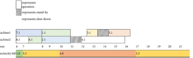
DOI: 10.4236/jep.2017.810066 1038 Journal of Environmental Protection Flow shop processing involves constant sequences of initial, standard, steady, and nonpermutable production, such as that of steel, optoelectronics, and metal, which are common in real-world situations [2][3]. To offer widely ap-plication, Linn and Zhang [4] indicated that FFS scheduling applies to tradi-tional flow shop situations. The attempted problem is excellently solved. However, the energy consumption of machines affects the efficiency and qual-ity of production; for instance, increased on-peak electricqual-ity consumption of machines causes an increase in temperature, wearing of parts, and improper manual operation. The time-of-use (TOU) tariff is a common used for adjust-ing peak power consumption worldwide. Generally, the billadjust-ing period is di-vided into on-peak hours, mid-peak hours, and off-peak hours. The electricity costs during the on-peak period are the highest, whereas those during the off-peak period are the lowest. Moreover, machines can be switched to opera-tion, standby, and shutdown modes for preventing unnecessary energy was-tage.
As for trade-off of energy saving method, Ribas et al. [5] demonstrated that enterprises added machines to certain stages, thus enhanced production effi-ciency and customer satisfaction. An energy-efficient mathematical model for solving FFS scheduling problems and multiobjective optimization to minimize the makespan and total energy consumption [6]. The experimental results showed that the relationship between the makespan and energy consumption may be conflicting. A proposed energy-saving decision is useful for minimizing energy consumption. To minimize trade-off of earliness and tardiness in a prac-tical production environment, Huang et al. [7] developed a farness particle swarm optimization (FPSO) algorithm for solving reentrant two-stage multi-processor flow shop scheduling problems.
house-DOI: 10.4236/jep.2017.810066 1039 Journal of Environmental Protection holds can alter their electricity consumption in response to varying prices and incentives; thus, a consumer may reduce electricity costs by more than 25%. Different values of the weighting factor (α) provide varying costs. According to the α values and their preferences, consumers can choose their electricity costs. FFS scheduling can save energy and lower manufacturing costs by clean tech-nologies, environmental policy, reducing the completion time and inventory in industrial environments.
Energy-saving models are created for important issues, Mouzon and Yildirim [12] developed operational methods for minimizing the energy consumption of manufacturing equipment and total completion time. The energy used in processes can be saved by turning off nonbottleneck (i.e., underutilized) ma-chines or equipment when they are idle for a certain period of time. In particu-lar, an analysis indicated that the proposed dispatching methods are effective in reducing the energy consumption of underutilized manufacturing equipment. Therefore, a production manager has a set of nondominated solutions (i.e., a set of efficient solutions) that he or she can use for determining the most efficient production sequence; moreover, they minimize the total energy consumption while optimizing the total completion time. Fang et al. [13] developed a new mathematical programming model for flow shop scheduling problems to mi-nimize the peak power load, energy consumption, and associated carbon foot-print along with the cycle time. In a flow shop with two machines producing various parts, the operation speed was considered an independent variable, which can be changed to affect the peak load and energy consumption. The results dem-onstrated that the proposed approach enables determining near-optimal sche-dules for achieving energy-saving goals. Tibi and Arman [14] developed a ma-thematical linear programming model to optimize the decision-making for managing a cogeneration facility as a potential clean-development mechanism project in a hospital in Palestine. The model optimized the cost of energy and the cost of installation of a small cogeneration plant under constraints on elec-tricity-and-heat supply and demand balances. The results proved the efficiency of the proposed method. He et al. [15] demonstrated that the environmental load resulting from the energy consumption of machine tool systems is broadly recognized. Improving scheduling saves energy, facilitates efficient use of ma-chine tools, and reduces energy consumption by idle equipment. One proposed energy-saving optimization method involves machine tool selection and a series of machine operations for flexible job shops. The method was designed to reduce the energy consumption of machine operations, and the scheduling was aimed at reducing the unused power consumption of machine tools. The current study investigated how to develop and use clean technologies like non-tardy proce-dures for scheduling the use of parallel machines to maintain practical produc-tion for environmental protecproduc-tion.
DOI: 10.4236/jep.2017.810066 1040 Journal of Environmental Protection energy-aware scheduling of manufacturing processes by using advanced plan-ning and scheduling, a mathematical model for optimally planplan-ning energy sav-ing for a given schedule. The new approach relies on the MIP model, where the reference schedule is modified to account for energy consumption without changing the jobs’ assignments and sequencing provided by the reference sche-dule. The results demonstrated that a commercial MIP solver and an original MIP heuristic are applicable in practical production.
Enumeration and heuristic methods have been applied for energy saving in previous studies [10]. Integer programming, branch and bound programming, and MIP are the most widely used enumeration methods that can provide ap-propriate solutions. However, high computational times limit the applicability of enumeration methods to small-scale problems [17]. Thus, heuristics such as the genetic algorithm, simulated annealing algorithm, and ant colony optimization algorithm are commonly used for solving energy-saving problems. Lian [18] ob-tained the average relative error rates of −28.20% and 60.25% for a combined local and global PSO algorithm against PSO and genetic algorithms, respectively. Zhang et al.[19] presented an I-ATTPSO algorithm with an average effective-ness improvement rate of −14% in small-scale problems and 55% in large-scale problems. Liu et al.[20] obtained an average relative error rate of 0.65% for the PSO-EDA_PI algorithm against other algorithms. Zhao et al.[21] found the av-erage relative error rate of their proposed logistic dynamic PSO algorithm against other algorithms to be approximately 1.19% - 2.39%.
In many industrialized countries, manufacturing industries pay stratified electricity charges depending on the time of the day (i.e., on-peak, mid-peak, and off-peak hours) [22]. China saves energy concerning the impact of internal industrial configuration in terms of size and ownership structure on aggregate energy intensity [23]. Besides, Germany property owners can deduce where they should ideally invest in order to optimize the energy efficiency of their building stock sustainably [24]. By contrast, the emerging smart grid concept may de-mand that industries pay real-time hourly electricity costs for the efficient usage of energy. To enable decision makers to apply feasible solutions for resolving unrelated parallel machine scheduling problems, Moon et al.[25] developed an energy-efficient method by using the weighted sum objective of production scheduling and electricity usage. Reliability models using a hybrid genetic algo-rithm along with their blank job insertion algoalgo-rithm consider the energy cost aspect of the problem with the objective function of optimizing the weighted sum of two criteria: the minimization of the production makespan and the mi-nimization of time-dependent electricity costs. The results demonstrated its performance in simulation experiments in practical production.
DOI: 10.4236/jep.2017.810066 1041 Journal of Environmental Protection proposed a mathematical model for minimizing energy consumption costs for single machine production scheduling during production processes. The job processing time consists of the starting time, idle time, and times when the ma-chine must be shut down, turned on, and turned off. The proposed mathemati-cal model enables the operation manager to implement the least expensive pro-duction scheduling during a propro-duction shift. To obtain feasible solutions by using a genetic algorithm, this study also determined whether the heuristic solu-tion provides the minimum cost and optimal schedule for minimizing energy costs. In addition, an analytical solution was applied to generate the optimal so-lution. Moreover, analytical solutions and heuristic solutions were compared, and the heuristic solution is considered preferable for larger problems. The re-sults indicate that significant reductions in energy costs can be achieved by avoiding high-energy price periods. The results have a positive environmental effect by reducing energy consumption during peak periods, thereby increasing the possibility of reducing CO2 emissions from power generator sites. Although a genetic algorithm can efficiently solve energy-saving problems and prevent en-trapment at a local optimum, the current study improves the solving process for enhancing performance in practical production and environmental protection.
By applying the nontardy constraint to practical production, the current study attempted to minimize makespan costs. A Cmax minimization genetic algorithm (CGA) and energy minimization genetic algorithm (EGA) are proposed for use in the first stage of solving two-stage multiprocessor flow shop scheduling prob-lems and minimizing makespan costs. Furthermore, an adjusted Cmax minimi-zation genetic algorithm (ACGA) and adjusted energy minimiminimi-zation genetic al-gorithm (AEGA) used in the second stage were compared for obtaining superior solutions and aiding enterprises in increasing profits and lowering overhead costs. The current study compared the proposed solution with two reported so-lutions that yielded comparable improvements.
The remainder of the paper is organized as follows: In Section 2, the FFS is formulated. In Section 3, the basic algorithms are introduced briefly. Then, the framework of energy-saving genetic algorithm for solving the FFS is proposed in Section 4. The influence of parameter setting is investigated based on design of experiment testing in Section 4, and computational results and comparisons are provided as well. Finally, we end the paper with some conclusions in Section 5.
2. Problem Definition
DOI: 10.4236/jep.2017.810066 1042 Journal of Environmental Protection Figure 1. State of machine process.
chart of the attempted problem.
The FFS problem provides multiple identical parallel machines at each station for increasing capacity and reducing costs in practical production. One machine at every station can be selected for each job and the process begins from the first station. After the final job is completed in the second stage, all jobs are com-pleted.
The scope and constraints of this study are demonstrated as follows: 1) Number of jobs, machines and stages are known.
2) Processing time of each job on each machine is known and constant. 3) Each machine in each stage can only process one job simultaneously. 4) The sequence through which jobs pass through machines may differ with the sequence of machine receiving job.
5) Jobs cannot be preempted.
6) There is no permutation, or machine breakdown. 7) The job ready time is 0.
8) Machines can switch into operation, stand-by, and shut-down.
2.1. Notation
T = total period set, all jobs in this study
M = total parallel machines at stage i, all machines in this study D = due date set, all jobs completed dates in this study
J = job set, all jobs waiting for scheduling in this study
K = stage set, all stages in this study
max
C = the maximal completion time of all jobs
j
d = the due date of job Jj
jkm
C = the completion time of job Jj processed in the m-th machine at the
k-th stage jkm
S = the starting time of job Jj processed in the m-th machine at the k-th stage
jkm
P = the processing time of job Jj processed in the m-th machine at the
k-th stage O t
E = the turn-on energy consumption of all machines at t-th time
I t
E = the stand-by energy consumption of all machines at t-th time
R t
E = the working energy consumption of all machines at t-th time
O km
DOI: 10.4236/jep.2017.810066 1043 Journal of Environmental Protection
I km
e = the stand-by energy consumption in the m-th machine at the k-th stage R
jkm
e = the working energy consumption of job Jj processed in the m-th machine at the k-th stage
t
EP = the electricity bill of different time period
jkmt
α = indicator of whether job Jj is scheduled at the k-th stage in m-th machine at t-th time (αjkmt = (0, 1); if αjkmt = 1, job Jj is processed at the
k-th stage in m-th machine at t-th time; otherwise αjkmt = 0) jkmt
β = indicator of whether job Jj is assigned at the k-th stage in m-th machine at t-th time (αjkmt = (0, 1); if αjkmt = 0, job Jj is processed at the
k-th stage in m-th machine at t-th time; otherwise αjkmt = 1)
kmt
Y = indicator of whether at the k-th stage the m-th machine turned on at
t-th time (Ykmt = (0, 1); if Ykmt = 1, the m-th machine was turned on at t-th time; otherwise Ykmt = 0)
kmt
δ = indicator of whether at the k-th stage the m-th machine turned off at
t-th time (δkmt = (0, 1); if δkmt = 0, the m-th machine was turned off at t-th time; otherwise δkmt = 1)
2.2. Mathematical Model
1) Objective function
(
)
min
∑
t T∈ EP Et tR+EtI +EtO (1) Equation (1) is the objective formulation and is primarily designed for mini-mizing energy consumption costs, such as those during operation, standby mode, and working. This equation measures the common criterion of the com-pletion of all jobs and aids enterprises in improving the energy consumption and efficiency of production scheduling.2) Total energy consumption
,
I I
t j J k K m M jkmt kmt km
E =
∑ ∑ ∑
∈ ∈ ∈ β δ e t∈T (2) ,R R
t j J k K m M jkmt jkm
E =
∑ ∑ ∑
∈ ∈ ∈ α e t∈T (3)O O
t m M kmt km
E =
∑
∈ γ e (4) Equation (2) is the standby total energy consumption of all machines at thet-th time. Equation (3) is the total energy consumption of all machines in the
t-th time period. Equation (4) is the turn-on total energy consumption of all machines in the t-th time period.
3) Completion time of job
, , ,
jkm j
C ≤d j∈J k∈K m∈M (5)
, , , ,
jkm jkm jkm
C =S +P j∈J k∈K m∈M t∈T (6)
( )1 , , ,
jkm j km
C ≤S + j∈J k∈K m∈M (7)
( 1) , , ,
jkm k m
C ≤S + j∈J k∈K m∈M (8)
DOI: 10.4236/jep.2017.810066 1044 Journal of Environmental Protection is the completion time of job j by the m-th machine at the k-th stage and equals the starting time plus the processing time. Equation (7) is the completion time of job j by the m-th machine at the k-th stage and is no longer than the starting time of job (j + 1) for the m-th machine at the k-th stage. Equation (8) is the completion time of job j by the m-th machine at the k-th stage and is no longer than the starting time of job j for the m-th machine at the (k + 1)-th stage. Be-cause of continuous production, the processing time prolongs the completion time and consumes energy. Therefore, minimizing energy consumption can re-main the primary objective of machines for further production.
4) The constraints of job processing
1, , , jkmt
m M∈
α
= j=J k∈K t∈T∑
(9)1, , , kmt kmt k K m M t T
γ +δ ≤ ∈ ∈ ∈ (10) , , , ,
jkmt kmt j J k K m M t T
α =δ ∈ ∈ ∈ ∈ (11)
Equation (9) controls all jobs during each stage and ensures that they are processed only once. Furthermore, Equation (10) controls the m-th machine and ensures that only one job can be processed by it. Finally, Equation (11) deter-mines whether the m-th machine is turned off at the t-th time (δkmt = (0, 1); if
kmt
δ = 0, the m-th machine was turned off at t-th time; otherwise δkmt = 1.
3. Concept of Energy-Saving Genetic Algorithm Solving
Procedure
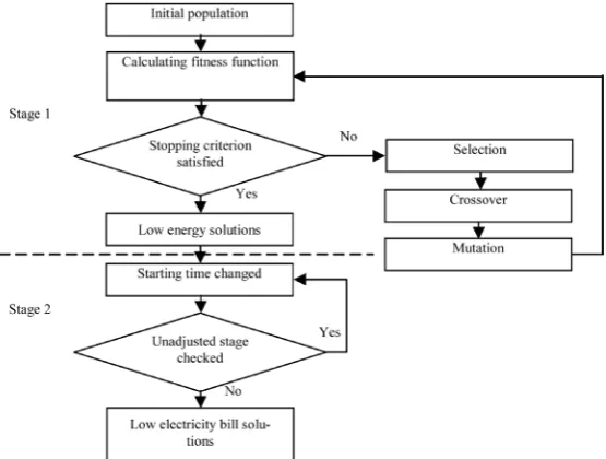
[image:8.595.237.515.494.704.2]According to FFk|EP State EC Tt, | | j=0, this study constructed energy-saving genetic algorithm (ESGA) using two-stage solving procedures: a genetic algo-rithm for maximizing the makespan and another for minimizing energy con-sumption in the second stage. Figure 2 demonstrates the starting time of solu-tions applied in the first stage to avoid on-peak hours.
DOI: 10.4236/jep.2017.810066 1045 Journal of Environmental Protection
3.1. The First Stage of ESGA
This study utilized two genetic algorithms for solving problems: the CGA for minimizing the makespan and calculating the electricity cost and EGA for de-termining low energy consumption scheduling and calculating the electricity cost concurrently [6]. The procedures of the proposed method are demonstrated as follows:
3.1.1. Encoding
According to Dai et al.[6], a job set, stage set, and machine set (
s
=
1, 2,
,
k
) are present at each stage. This study formulated FFS scheduling as a genetic ma-trix in which the columns are jobs and stages are rows.1,1 1,
1,1
,1 ,
j
k j
k k j
a
a
A
a
a
a
× =
(12)The am n,
(
m=1, 2,, ,k n=1, 2,,j)
is a real number in the interval (1,s
M ). am n, indicates which machine processes job j, and the decimal indicates the processing sequence; the lower the decimal is, the earlier the job is processed. A coding matrix represents a chromosome in which k× j genes are present.
1,1, 1,2, , 1,j, 2,1, 2,2, , k j,
a a a a a a
(13) For example, in FFS scheduling, the coding matrix consists of three stages, in which there are two machines and eight jobs to be processed.
1.301 2.533 1.415 2.76 1.824 2.351 1.113 2.204
1.261 1.997 2.442 1.528 2.609 1.016 2.224 2.185
1.518 1.635 2.254 2.965 2.753 1.378 2.181 2.156
A
=
(14)Row 1 represents processing conditions of the first stage. The a1,1=1.301 means J1 processed in machine 1, a1,2=2.533 means J2 processed in ma-chine 2, and a1,3=1.145 means J3 processed in machine 1. The decimal of
1,1
a is 0.301smaller than 0.415 of a1,3, which represents a1,1 is processed earli-er than a1,3.
[
]
1.301, 2.533, 1.415, 2.76, 1.824, 2.351,1.113, 2.204, 1.261,
1.997, 2.442, 1.528, 2.609, 1.016, 2.224, 2.185, 1.518, 1.635,
2.254, 2.965, 2.753, 1.378, 2.181, 2.156
(15)
3.1.2. Initial Population
The initial solution is the first population of a genetic algorithm. Generally, two methods can generate initial solutions: one is randomly generated and other re-quires research. The scale of the initial population affects the efficiency and quality of solutions. A random initial solution was used in this study.
3.1.3. The Fitness Function
DOI: 10.4236/jep.2017.810066 1046 Journal of Environmental Protection
( )
max 1 f x
C
= (16) The fitness function of EGA is as below:
( )
(
1)
T I O
t t t t t T
f x
EP E E E
∈
=
+ +
∑
(17)3.1.4. Selection
The algorithm selects a favorable parent from chromosomes and proceeds with crossover and mutation. Each chromosome has a fitness value, which determines the possibility for crossover and mutation. This study adopted roulette wheel se-lection.
3.1.5. Crossover
The proposed algorithm partially exchanges two chromosomes. In this study, the exchange rate was set as, which is a rounded-up approximation of the quantity of exchanged chromosome multiplied by the exchange rate. If the quantity of exchanged chromosome is odd, then one chromosome is added to the total chromosomes and the quantity becomes even. The exchange rate was set at 0.9, and this study adopted a two-point crossover method to solve the considered problem.
3.1.6. Crossover
Mutation can generate multiple and various children. A mutation rate of Pm was set in this study. The proposed method arbitrarily generates a probability value. If the value is below the mutation rate, mutation occurs. The mutation rate was set at 0.1. The mutation rate is uniformly distributed from 0 to 1. If the rate becomes 1, the proposed algorithm regenerates an interval of real numbers (1, Ms + 1).
3.2. The Second Stage of ESGA
Although the genetic algorithm generates scheduling with lower electricity costs, some jobs still generate high electricity costs. The solutions generated from the GCA and EGA in the first stage were adjusted using the ACGA, and problems in the second stage were solved using the AEGA to avoid high-energy price pe-riods.
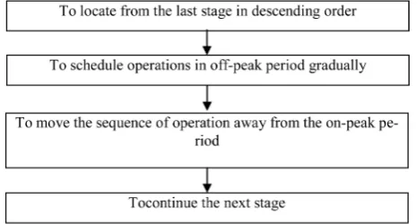
The adjustment rule begins from the final stage and proceeds in descending order. The proposed approach organizes the operations into the final order. The method gradually schedules operations in the off-peak period and moves the sequence of operation away from the on-peak period until all jobs are scheduled. Figure 3 illustrates the flow chart.
3.3. A Brief Example
DOI: 10.4236/jep.2017.810066 1047 Journal of Environmental Protection factory working period is from 6 a.m. to 10 p.m. on each day. Table 1 shows the operation time:
Table 2 shows the consumed energy of machines. The starting time of the machines is assumed to be short with sudden turn-on energy consumption.
Table 3 shows the electricity costs of every time period. The parameters of the proposed method are as follows: initial population, 30; exchange rate, 0.9; muta-tion rate, 0.1; and stopping criterion, 300 iteramuta-tions.
3.3.1. The First Stage of ESGA
Figure 4 shows the computational result using CGA, and the electricity bill is NT$ 3277.8.
[image:11.595.206.540.428.593.2]Figure 3. Flow chart of solving procedure of ESGA.
Table 1. The operation working time.
Jobs The working time of jobs at different stages
Stage 1 Stage 2 Stage 3
1 Hour 3 4 1
2 Hour 3 2 2
3 Hour 1 2 3
4 Hour 4 2 3
5 Hour 2 2 0.5
6 Hour 0.5 1 1.5
7 Hour 2 0.5 1
[image:11.595.207.540.625.697.2]8 Hour 1.5 2 1.5
Table 2. The operation working time.
Conditions of machines Stage 1 Stage 2 Stage 3
Stand-by (kW) 3 7 6
Operation (kW) 8 18 17
Turn-on (kW) 4 10 8
DOI: 10.4236/jep.2017.810066 1048 Journal of Environmental Protection
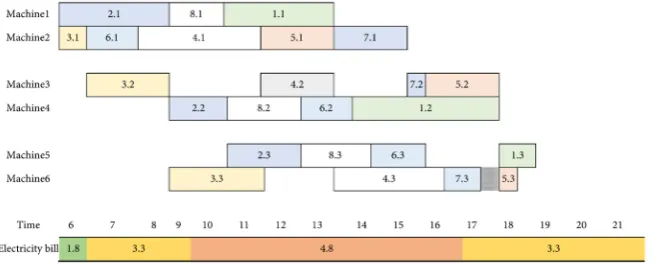
Figure 5 shows the computational result using EGA, and the electricity bill is NT$ 2900.6.
3.3.2. The Second Stage of ESGA
The adjustment rule begins from the final stage and proceeds in descending or-der. The proposed approach organizes operations into the final oror-der. The me-thod gradually schedules operations in the off-peak period and moves the se-quence of operation away from the on-peak period until all jobs are scheduled. Figure 6 shows the computational result obtained using the ACGA and the electricity cost is NT$ 2929.7.
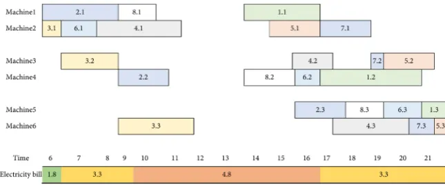
Figure 7 the computational result using AEGA, and the electricity bill is NT$ 2807.4.
[image:12.595.216.537.438.569.2]Table 4 lists four computational results obtained using the CGA as the
[image:12.595.207.539.619.734.2]Figure 4. The Gantt chart of computational result using CGA.
Figure 5. The Gantt chart of computational result using EGA.
Table 3. The electricity bill of time periods.
Factory working period 6:00~20:00
Time period Summer electricity price (NT$)
Off-peak 6:00~7:00 1.8
Mid-peak 7:00~10:00 3.3
17:00~20:00 3.3
DOI: 10.4236/jep.2017.810066 1049 Journal of Environmental Protection Figure 6. The Gantt chart of computational result using ACGA.
[image:13.595.208.539.427.478.2]Figure 7. The Gantt chart of computational result using AEGA.
Table 4. Comparison of electricity bills.
CGA EGA ACGA AEGA
Electricity bills (NT$) 3277.8 2900.6 2929.7 2807.4
Comparison costs ratio 1 0.88 0.89 0.86
benchmark for comparison. According to Table 4, applying the CGA generates the highest electricity cost, because it neglects the costs of standby, shutdown, and different time periods. Furthermore, the EGA considers different conditions of machines and can lower the electricity cost; however, jobs are processed in the on-peak period. The proposed method using ESGA can efficiently avoid processing jobs in the on-peak period. Moreover, ESGA can lower the electricity cost by up to 11% and 14%, respectively, compared with the CGA. The results demonstrate higher energy saving with the AEGA than with the CGA, EGA, and ACGA.
4. Computational Experiments
DOI: 10.4236/jep.2017.810066 1050 Journal of Environmental Protection consumption of machines, processing time of jobs, and due dates. For the con-sidered problems, the number of jobs was 30, 60, or 90; the type of stage was 3 or 5; and the number of machines in the two stages = 6, 9. Table 2 and Table 5 show the energy consumption of machines. Moreover, the processing time of jobs was limited within U [2] [9]; the unit time was 30 minutes; the factory working period was from 6 a.m. to 10 p.m. on each day; and the electricity costs of various time periods are shown in Table 3. The formula of the due date
(
1)
1(
1(
1)
0.25)
k i i
TF = P k
−
∑
+ + ∗ , among which the Pi represents the average processing time of machines, and TF is the tardy factor; Type I was 0.3 and Type II was 0.5. The working duration per day was assumed to be 16 hours. Therefore, when the formula of the due date provided a duration of 20 hours, the due date was estimated to be 2 days. Finally, the parameters of the genetic algorithms were set on the basis of a pretest to improve the results; specifically, the initial population was 30; the exchange rate was 0.9; the mutation rate was 0.1; and the stopping criterion was 500 iterations.4.1. Analysis of Effectiveness
To assess the effectiveness of the proposed algorithm in solving the considered problems, 12 conditions were applied to randomly test 30 generated problem sets; specifically, the number of jobs was 30, 60, or 90; the type of stage was 3 or 5; and the number of machines in the two stages was 6 or 9. Table 6 provided a comparison of the average solutions and average solving times of the CGA, EGA, ACGA, and AEGA for efficacy analysis under Type I of slacker due dates.
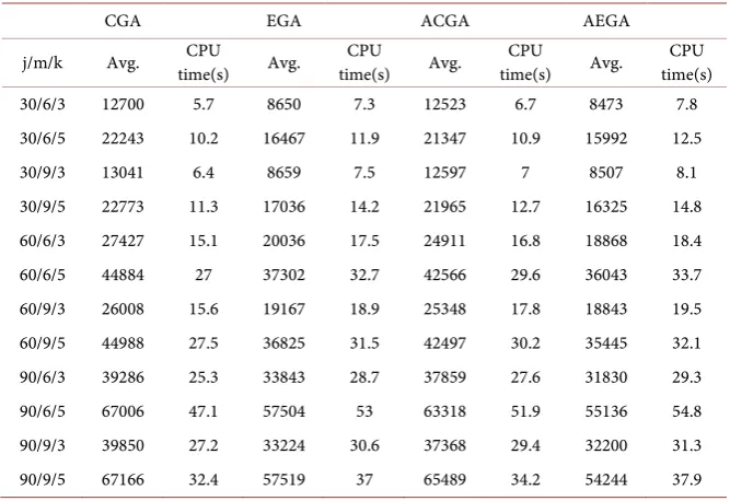
Table 7 provided a comparison of the average solutions and average solving times of the CGA, EGA, ACGA, and AEGA for efficacy analysis under Type II of non-slacker due dates.
Table 6 and Table 7 illustrate that for different due dates, the cost of energy consumption is lower for the ACGA and AEGA than for the CGA. Type I has slacker due dates than those of Type II, indicating that the EGA and AEGA pro-vide superior solutions. A data set of 30/6/5 has the same due date as that of Type I and Type II; therefore, the improvement is not remarkable. The CGA calculates the electricity cost for the minimal makespan; therefore, the CGA and ACGA might not provide superior solutions in the Type I condition. Table 8 show comparison cost ratios for electricity costs obtained using all methods un-der Type I of slacker due dates.
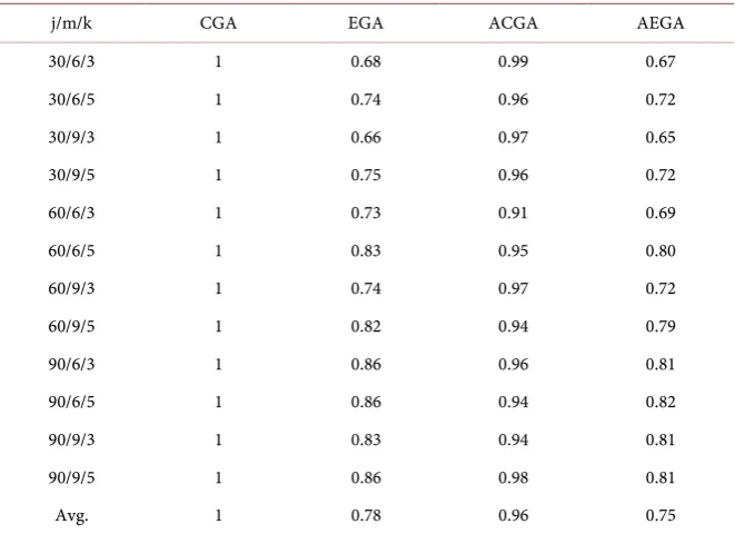
Table 8 and Table 9 show comparison cost ratios for electricity costs obtained using all methods under Type I of non-slacker due dates.
Table 5. The energy consumption during three time periods of 5-stage machines.
Conditions of machines Stage 1 Stage 2 Stage 3 Stage 4 Stage 5
Stand-by (kW) 3 7 6 6 5
Operation (kW) 8 18 17 15 14
DOI: 10.4236/jep.2017.810066 1051 Journal of Environmental Protection Table 6. The effectiveness of time window Type I.
CGA EGA ACGA AEGA
j/m/k Avg. time(s) CPU Avg. time(s) CPU Avg. time(s) CPU Avg. time(s) CPU
30/6/3 12673 5.8 8558 7.1 12471 6.6 8314 7.5
30/6/5 22519 9.9 15957 12.1 20681 11.3 15438 12.6
30/9/3 13173 6.4 8721 7.6 12405 7.2 8616 8.2
30/9/5 23098 11.4 16516 13.8 20893 12.2 15706 14.4 60/6/3 26545 15.3 19420 17.6 24187 16.5 18242 18.2 60/6/5 44668 27.4 37244 32.4 42057 30.3 34822 33.2 60/9/3 25903 16 18763 19 24779 18.2 18412 19.7 60/9/5 44647 27 36474 31.7 42664 29.9 34236 32.1 90/6/3 39398 25.7 31909 29.4 37783 28.5 29634 30.8 90/6/5 65787 48.5 57154 53.9 62155 51.3 53657 55 90/9/3 40014 26.7 31456 30.5 37869 29.7 30431 31.1 90/9/5 66557 31.5 57340 37.4 64741 33.6 53933 38
[image:15.595.206.540.359.588.2]Remarks: The unit cost is NT$.
Table 7. The effectiveness of time window Type II.
CGA EGA ACGA AEGA
j/m/k Avg. time(s) CPU Avg. time(s) CPU Avg. time(s) CPU Avg. time(s) CPU
30/6/3 12700 5.7 8650 7.3 12523 6.7 8473 7.8
30/6/5 22243 10.2 16467 11.9 21347 10.9 15992 12.5
30/9/3 13041 6.4 8659 7.5 12597 7 8507 8.1
30/9/5 22773 11.3 17036 14.2 21965 12.7 16325 14.8 60/6/3 27427 15.1 20036 17.5 24911 16.8 18868 18.4 60/6/5 44884 27 37302 32.7 42566 29.6 36043 33.7 60/9/3 26008 15.6 19167 18.9 25348 17.8 18843 19.5 60/9/5 44988 27.5 36825 31.5 42497 30.2 35445 32.1 90/6/3 39286 25.3 33843 28.7 37859 27.6 31830 29.3 90/6/5 67006 47.1 57504 53 63318 51.9 55136 54.8 90/9/3 39850 27.2 33224 30.6 37368 29.4 32200 31.3 90/9/5 67166 32.4 57519 37 65489 34.2 54244 37.9
Remarks: The unit cost is NT$.
Table 8 and Table 9 illustrate that the EGA, ACGA, and AEGA yielded lower electricity costs than did the CGA. Moreover, the AEGA provided solutions su-perior to those of the ACGA method in terms of effectiveness.
4.2. Analysis of Robustness
DOI: 10.4236/jep.2017.810066 1052 Journal of Environmental Protection Table 8. The comparison costs ratio of electricity bills of time window Type I.
j/m/k CGA EGA ACGA AEGA
30/6/3 1 0.68 0.98 0.66
30/6/5 1 0.71 0.92 0.69
30/9/3 1 0.66 0.94 0.65
30/9/5 1 0.72 0.90 0.68
60/6/3 1 0.73 0.91 0.69
60/6/5 1 0.83 0.94 0.78
60/9/3 1 0.72 0.96 0.71
60/9/5 1 0.82 0.96 0.77
90/6/3 1 0.81 0.96 0.75
90/6/5 1 0.87 0.94 0.82
90/9/3 1 0.79 0.95 0.76
90/9/5 1 0.86 0.97 0.81
Avg. 1 0.77 0.94 0.73
Table 9. The comparison costs ratio of electricity bills of time window Type II.
j/m/k CGA EGA ACGA AEGA
30/6/3 1 0.68 0.99 0.67
30/6/5 1 0.74 0.96 0.72
30/9/3 1 0.66 0.97 0.65
30/9/5 1 0.75 0.96 0.72
60/6/3 1 0.73 0.91 0.69
60/6/5 1 0.83 0.95 0.80
60/9/3 1 0.74 0.97 0.72
60/9/5 1 0.82 0.94 0.79
90/6/3 1 0.86 0.96 0.81
90/6/5 1 0.86 0.94 0.82
90/9/3 1 0.83 0.94 0.81
90/9/5 1 0.86 0.98 0.81
Avg. 1 0.78 0.96 0.75
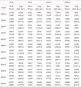
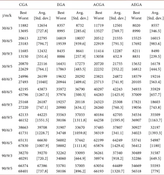
specifically, the number of jobs was 30, 60, or 90; the type of stage = 3, 5; and the number of machines in the two stages Ms = 6, 9. Table 10 and Table 11 pro-vide a comparison of the average solutions, optimal solutions, and poorest solu-tions calculated using the CGA, EGA, ACGA, and AEGA in the analysis of ro-bustness.
[image:16.595.208.539.358.598.2]DOI: 10.4236/jep.2017.810066 1053 Journal of Environmental Protection Table 10. The robustness of time window Type I.
CGA EGA ACGA AEGA
j/m/k Worst Best [Std. dev.] Avg. Worst Best [Std. dev.] Avg. Worst Best [Std. dev.] Avg. Worst Best [Std. dev.] Avg.
30/6/3 11330 12687 [492.6] 12202 8136 9105 [356.6] 8991 11083 12249 [422.5] 11693 7964 8832 [307] 8507
30/6/5 21853 23085 [677.9] 22469 16430 18034 [537.5] 17232 21090 22272 [427.3] 21836 15082 16512 [420.3] 16030
30/9/3 11336 13170 [684.2] 12253 8521 9118 [353.6] 8819 10534 12430 [686.5] 11707 8100 8864 [497] 8381
30/9/5 20937 23189 [862.1] 22169 16131 17282 [457.5] 16707 19170 22567 [1304.3] 21395 15434 16172 [295.2] 15805
60/6/3 24779 27195 [984.5] 25987 19118 20513 [653.2] 19822 23062 25432 [936.9] 24515 18267 19706 [646.8] 18945
60/6/5 42020 44735 [999.2] 43378 35442 36632 [676.3] 35805 39517 42368 [1065.6] 41239 34267 36301 [758.8] 35256
60/9/3 24565 27261 [1149.6] 25913 18209 19711 [594.7] 18920 24124 25826 [646.8] 24719 17415 18753 [370.2] 18288
60/9/5 43167 46538 [1209.4] 44852 35305 37244 [881.6] 36377 41856 43784 [865.1] 42481 33707 36761 [845.2] 35112
90/6/3 38541 40956 [907.9] 39749 32015 34513 [955.7] 33263 37124 38134 37712 [438] 27963 31085 [1161.7] 29877
90/6/5 65226 67744 [929.0] 66485 55357 57823 [913.8] 56175 61613 63426 [720.1] 62774 52056 54253 [889.5] 53456
90/9/3 39596 41817 [839.8] 40707 30663 31878 [436.2] 31270 35614 37759 [941.5] 37211 29920 31085 [416.2] 30545
90/9/5 65027 68482 [1270.9] 66754 55440 57461 [682.9] 56450 62526 66064 [1878.7] 64235 54006 55744 [674.4] 54620
Remarks: The unit cost is NT$.
causing the electricity cost to decrease partially. Thus, the robustness of the proposed method was fairly identified.
5. Computational Experiments
This study investigated the use of limited resources of parallel machines to pro-mote practical production and environmental protection. Ideal practical produc-tion for better energy using effective scheduling prevents processes from exces-sive energy consumption and energy price fluctuations. Recent studies on sus-tainable manufacturing focused on energy saving to reduce the unit production cost and environmental impacts.
DOI: 10.4236/jep.2017.810066 1054 Journal of Environmental Protection Table 11. The robustness of time window Type II.
CGA EGA ACGA AEGA
j/m/k Worst Best [Std. dev.] Avg. Worst Best [Std. dev.] Avg. Worst Best [Std. dev.] Avg. Worst Best [Std. dev.] Avg.
30/6/3 11882 13695 [727.8] 12654 8357 8995 [285.6] 8732 11719 13527 [769.7] 12501 8020 8990 [346.5] 8557
30/6/5 20613 23183 [794.7] 22795 16819 19539 [939.6] 18037 20512 22919 [791.5] 21555 15525 17692 [983.6] 16015
30/9/3 11685 13150 [551.6] 12432 8435 8886 [257.9] 8641 11414 13058 12287 652.9 8211 8831 [239.5] 8490
30/9/5 20870 22629 [764.1] 22116 16431 17863 [483.5] 17273 20720 22232 [552.2] 21755 15632 16812 [444.5] 16178
60/6/3 24996 27493 [1040] 26199 19632 20944 [409.6] 20292 23821 25713 [741.9] 24872 18579 20105 [563.4] 19216
60/6/5 42195 45796 [1267.5] 43873 35972 37976 [500.5] 36790 40297 44283 [1425.9] 42243 34933 37009 [657.7] 35929
60/9/3 25168 27220 [747.1] 26187 19257 20980 [634.1] 20118 24323 26260 [760.3] 25308 17821 19056 [743.8] 18603
60/9/5 42133 46152 [1551.5] 44225 35563 38106 [1311.8] 37033 40184 44258 [1595.9] 42705 34534 36907 [1163.7] 35509
90/6/3 38663 41731 [1228.7] 39708 31907 34748 [1059.8] 33670 37485 38319 [341.1] 37807 30927 34023 [1393.3] 32197
90/6/5 65131 67830 [1007.9] 66630 56002 58882 [1111.8] 57442 62199 65876 [1429.4] 64249 53741 56412 [1180] 54987
90/9/3 38270 40291 [720.2] 39270 32262 34060 [664.9] 33093 36261 38974 [918.2] 37340 30489 32286 [649.5] 31587
90/9/5 66374 68401 [737.8] 67386 55781 58106 [896.2] 57005 63054 66193 [1320.7] 64489 54669 56518 55593 [779]
Remarks: The unit cost is NT$.
According to the analysis, the CGA, EGA, ACGA, and AEGA can efficiently solve problems. The electricity cost ratio for the CGA, EGA, ACGA, and AEGA is 1:0.78:0.95:0.74, demonstrating that the AEGA can efficiently solve the prob-lem. The robustness test results show that the ACGA and AEGA of ESGA are affected by original solutions during adjustment procedures and partially reduce electricity costs. Thus, the robustness of the proposed method was appropriately identified. As a whole, the proposed method can lower electricity bills to fit green energy nowadays.
Finally, enterprises can adopt the proposed method for enhancing practical production in the flexible job shop scheduling environment and generate profits by fully exploiting the advantages of the method in the future. In addition, the proposed method can mitigate the environmental impact of manufacturing processes and protect environment at the same time.
References
DOI: 10.4236/jep.2017.810066 1055 Journal of Environmental Protection [2] Tongur, V. and Ülker, E. (2014) Migrating Birds Optimization for Flow Shop
Se-quencing Problem. Journal of Computer and Communications, 2, 142-147.
https://doi.org/10.4236/jcc.2014.24019
[3] Zabihzadeh, S.S. and Rezaeian, J. (2016) Two Meta-Heuristic Algorithms for Flexi-ble Flow Shop Scheduling ProFlexi-blem with Robotic Transportation and Release Time. Applied Soft Computing, 40, 319-330. https://doi.org/10.1016/j.asoc.2015.11.008
[4] Linn, R. and Zhang, W. (1999) Hybrid Flow Shop Scheduling: A Survey. Computers and Industrial Engineering, 37, 57-61.
https://doi.org/10.1016/S0360-8352(99)00023-6
[5] Ribas, I., Leisten, R. and Framiñan, J.M. (2010) Review and Classification of Hybrid Flow Shop Scheduling Problems from a Production System and a Solutions Proce-dure Perspective. Computers & Operations Research, 37, 1439-1454.
https://doi.org/10.1016/j.cor.2009.11.001
[6] Dai, M., Tang, D., Giret, A., Salido, M.A. and Li, W.D. (2013) Energy-Efficient Scheduling for a Flexible Flow Shop Using an Improved Genetic-Simulated An-nealing Algorithm. Robotics and Computer-Integrated Manufacturing, 29, 418-429.
https://doi.org/10.1016/j.rcim.2013.04.001
[7] Huang, R.H., Yu, S.C. and Kuo, C.W. (2014) Reentrant Two-Stage Multiprocessor Flow Shop Scheduling with Due Windows. The International Journal of Advanced Manufacturing Technology, 71, 1263-1276.
https://doi.org/10.1007/s00170-013-5534-4
[8] Mukund Nilakantan, J., Huang, G.Q. and Ponnambalam, S.G. (2015) An Investiga-tion on Minimizing Cycle Time and Total Energy ConsumpInvestiga-tion in Robotic Assem-bly Line Systems. Journal of Cleaner Production, 90, 311-325.
https://doi.org/10.1016/j.jclepro.2014.11.041
[9] Zhang, H., Zhao, F., Fang, K. and Sutherland, J.W. (2014) Energy-Conscious Flow Shop Scheduling under Time-of-Use Electricity Tariffs. CIRP Annals-Manufacturing Technology, 63, 37-40. https://doi.org/10.1016/j.cirp.2014.03.011
[10] Setlhaolo, D., Xia, X. and Zhang, J. (2014) Optimal Scheduling of Household Ap-pliances for Demand Response. Electric Power Systems Research, 116, 24-28.
https://doi.org/10.1016/j.epsr.2014.04.012
[11] Jin, W., Hu, Z. and Chan, C. (2017) An Innovative Genetic Algorithms-Based In-exact Non-Linear Programming Problem Solving Method. Journal of Environmen-tal Protection, 8, 231-249. https://doi.org/10.4236/jep.2017.83018
[12] Mouzon, G., Yildirim, M.B. and Twomey, J. (2007) Operational Methods for Mini-mization of Energy Consumption of Manufacturing Equipment. International Journal of Production Research, 45, 4247-4271.
https://doi.org/10.1080/00207540701450013
[13] Fang, K., Uhan, N., Zhao, F. and Sutherland, J.W. (2011) A New Approach to Scheduling in Manufacturing for Power Consumption and Carbon Footprint Re-duction. Journal of Manufacturing Systems, 30, 234-240.
https://doi.org/10.1016/j.jmsy.2011.08.004
[14] Tibi, N.A. and Arman, H. (2007) A Linear Programming Model to Optimize the Decision-Making to Managing Cogeneration System. Clean Technologies and En-vironmental Policy, 9, 235-240. https://doi.org/10.1007/s10098-006-0075-2
[15] He, Y., Li, Y.F., Wu, T. and Sutherland, J.W. (2015) An Energy-Responsive Opti-mization Method for Machine Tool Selection and Operation Sequence in Flexible Machining Job Shops. Journal of Cleaner Production, 87, 245-254.
DOI: 10.4236/jep.2017.810066 1056 Journal of Environmental Protection [16] Bruzzone, A.A.G., Anghinolfi, D., Paolucci, M. and Tonelli, F. (2012) Energy-Aware
Scheduling for Improving Manufacturing Process Sustainability: A Mathematical Model for Flexible Flow Shops. CIRP Annals-Manufacturing Technology, 61, 459-462. https://doi.org/10.1016/j.cirp.2012.03.084
[17] Shao, W., Pi, D. and Shao, Z. (2017) Memetic Algorithm with Node and Edge His-togram for No-Idle Flow Shop Scheduling Problem to Minimize the Makespan Cri-terion. Applied Soft Computing, 54, 164-182.
https://doi.org/10.1016/j.asoc.2017.01.017
[18] Lian, Z.G. (2010) A Local and Global Search Combine Particle Swarm Optimization Algorithm for Job-Shop Scheduling to Minimize Makespan. Discrete Dynamics in Nature and Society, 2010, Article ID 838596, 11 p.
[19] Zhang, C.S., Ning, J. and Ouyang, D. (2010) A Hybrid Alternate Two Phases Par-ticle Swarm Optimization Algorithm for Flow Shop Scheduling Problem. Comput-ers and Industrial Engineering, 58, 1-11. https://doi.org/10.1016/j.cie.2009.01.016
[20] Liu, H.C., Gao, L. and Pan, Q. (2011) A Hybrid Particle Swarm Optimization with Estimation of Distribution Algorithm for Solving Permutation Flowshop Schedul-ing Problem. Expert Systems with Applications, 38, 4348-4360.
https://doi.org/10.1016/j.eswa.2010.09.104
[21] Zhao, F., Tang, J., Wang, J. and Jonrinaldi, J. (2014) An Improved Particle Swarm Optimisation with a Linearly Decreasing Disturbance Term for Flow Shop Sche-duling with Limited Buffers. International Journal of Computer Integrated Manu-facturing, 27, 488-499. https://doi.org/10.1080/0951192X.2013.814165
[22] Li, T., Castro, P.M. and Lv, Z. (2017) Life Cycle Assessment and Optimization of an Iron Making System with a Combined Cycle Power Plant: A Case Study from Chi-na. Clean Technologies and Environmental Policy, 19, 1133-1145.
https://doi.org/10.1007/s10098-016-1306-9
[23] Ma, B. and Yu, Y. (2017) Industrial Structure, Energy-Saving Regulations and Energy Intensity: Evidence from Chinese Cities. Journal of Cleaner Production, 141, 1539-1547. https://doi.org/10.1016/j.jclepro.2016.09.221
[24] Peyramalea, V. and Wetzelb, C. (2017) Analyzing the Energy-Saving Potential of Buildings for Sustainable Refurbishment. Procedia Environmental Sciences, 38, 162-168. https://doi.org/10.1016/j.proenv.2017.03.098
[25] Moon, J.Y., Shin, K. and Park, J. (2013) Optimization of Production Scheduling with Time-Dependent and Machine-Dependent Electricity Cost for Industrial Energy Efficiency. The International Journal of Advanced Manufacturing Technol-ogy, 68, 523-535. https://doi.org/10.1007/s00170-013-4749-8
[26] Shrouf, F., Ordieres-Mere, J., Garcia-Sanchez, A. and Ortega-Mier, M. (2014) Op-timizing the Production Scheduling of a Single Machine to Minimize Total Energy Consumption Costs. Journal of Cleaner Production, 67, 197-207.
https://doi.org/10.1016/j.jclepro.2013.12.024
Submit or recommend next manuscript to SCIRP and we will provide best service for you:
Accepting pre-submission inquiries through Email, Facebook, LinkedIn, Twitter, etc. A wide selection of journals (inclusive of 9 subjects, more than 200 journals)
Providing 24-hour high-quality service User-friendly online submission system Fair and swift peer-review system
Efficient typesetting and proofreading procedure
Display of the result of downloads and visits, as well as the number of cited articles Maximum dissemination of your research work