Systemic Financial Risk Indicators and Securitised Assets: an Agent Based Framework

Munich Personal RePEc Archive

Systemic Financial Risk Indicators and

Securitised Assets: an Agent-Based

Framework

Mazzocchetti, Andrea and Lauretta, Eliana and Raberto,

Marco and Teglio, Andrea and Cincotti, Silvano

University of Genoa, University of Birmingham, University of

Genoa, University Ca’ Foscari of Venice, University of Genoa

24 October 2018

Online at

https://mpra.ub.uni-muenchen.de/89779/

Systemic Financial Risk Indicators and Securitised Assets: an Agent-Based

Framework

Andrea Mazzocchettia_{, Eliana Lauretta}b_{, Marco Raberto}a_{, Andrea Teglio}c,d_{, Silvano Cincotti}a

a

DIME-CINEF, Universit`a di Genova, Via Opera Pia 15, 16145 Genova, Italy

b

Department of Finance, Birmingham Business School, University of Birmingham, University House, Edgbaston Park Road, Birmingham B15 2TY, UK

c

Department of Economics, University Ca’ Foscari of Venice, Cannaregio 873, 30121 Venezia, Italy

d

Universitat Jaume I, Campus del Riu Sec, 12071 Castell´on, Spain

Abstract

The paper presents an agent-based model of a credit economy which includes a securitisation process and

a bailout mechanism for banks’ bankruptcies. Within this model’s framework banks are able to sell mortgages

to a Financial Vehicle Corporation, which finances its activity by creating Mortgage-Backed Securities and

selling them to a mutual fund. In turn, the mutual fund collects liquidity by selling shares to households

and remunerating them with a monthly interest rate. The impact of this mechanism is analysed by means

of computational experiments for different levels of securitisation propensities of banks. Furthermore, we

study a set of systemic risk indicators which have the aim to assess financial imbalances within the financial

system. Two of them are the mortgage-to-GDP ratio and the Capital Adequacy Ratio which are constructed

to detect only the in-balance sheet changes in banks’ credit exposure. We consider two additional indicators,

similar to the previous ones with the only difference that they are able to account also for the off-balance

sheet items. Moreover, we introduce a novel indicator, the so-called VUC indicator, which also targets the

off-balance assets. Results confirm that higher securitisation propensities weaken the financial stability of

banks with relevant effects on different sectors of the economy. Most important, the analysis of systemic risk

reveals the important issue of designing suitable systemic risk indicators for predicting incoming financial

crises, finding that an essential feature of these indicators should be to integrate banks’ off-balance sheet

assets.

Keywords: sytemic financial risk indicators, securitisation, housing market, agent-based models

JEL classification: C63, R31, G21, G23

Email addresses: [email protected](Andrea Mazzocchetti),[email protected](Eliana Lauretta),

Introduction

The paper contributes to the literature of macro-financial agent-based models, financial innovation and

systemic risk. The study aims to answer the question of why financial risk indicators, with a particular focus

on those detecting financial instabilities, remain only partially able to identify in time and quantify the actual

financial system risk exposure. The models applied so far for detecting financial imbalances (e.g. see Borio

and Lowe, 2002a; Misina and Tkacz, 2009; Barrell et al., 2010, among others) still present large errors in

their predicting power (ECB, 2011; Deghi et al., 2018).

We analyse five systemic risk indicators which have the aim to assess financial imbalances within the

financial system. Two of them are the well-known mortgage-to-GDP ratio and the Capital Adequacy Ratio1

(e.g. see Borio and Lowe, 2002a; Barrell et al., 2010), which are constructed to detect only the in-balance

sheet (in-BS) changes in credit exposure of the banking sector (CAR) and the financial system as a whole

(credit-to-GDP). We consider two additional indicators, similar to the previous ones with the only difference

that they are able to account also for the off-BS items. We call them adjusted mortgages-to-GDP and

adjusted CAR. Moreover, we introduce a last indicator, so-called VUC indicator (see Lauretta et al. (2016)),

which also targets the off-balance sheet (off-BS) assets.

Usually, banks decide to forward the off-BS items to the securitisation process to reduce the level of risk

exposure of their credit portfolio. We analyse these indicators and compare the in-BS and off-BS dimensions

in the context of the agent-based macroeconomic simulator Eurace (Cincotti et al., 2010, 2012a; Raberto

et al., 2012; Teglio et al., 2017). To the best of our knowledge, this is the first time that in-BS and off-BS

measures to detect financial imbalances are analysed and implemented in an agent-based economy.

Eurace reproduces an artificial macroeconomy integrating different sectors and markets populated by

heterogeneous and bounded rational agents. Each agent is characterised by a double-entry balance sheet (i.e.

the “balance sheet approach” described in Teglio et al. (2010)) which enables us to observe the debts-credits

dynamics in- and off-balance sheet and, thus to take account of those dynamics in the assessment of the

systemic financial risk. We use this model for its peculiarity to reproduce real-world economic dynamics in a

simplified but still rich way. In fact, it presents the ideal environment for the study of the out-of-equilibrium

and non-linear dynamics of the economy.

The version of Eurace presented here includes a housing market in the style of Ozel et al. (2016), and a

securitisation mechanism on the footprints of Mazzocchetti et al. (2018) and Lauretta (2018) that allows banks

to free up their balance sheets from risk-weighted assets and circumvent the prudential capital requirements.

A behavioural rule governs the model: the securitisation propensity. It is introduced as an exogenous

parameter and determines the level of banks’ resort on the securitisation. To higher values of the securitisation

propensity corresponds a higher resort to securitisation. Moreover, the model shows a bailout resolution

1

mechanism for banks’ bankruptcies, which foresees the banks’ rescue by means of government spending if

banks’ equity becomes negative (see Section 3.2 for more details).

In the aftermath of the crisis, the management of banks breakdowns has been a major concern for the

public institutions of most developed countries around the globe. In the last decade, sovereign States and

international organisations coped with the burden of the threat of banks’ failures and employed several policy

tools to bring back the economic system to a certain level of stability. Moreover, some financial institutions

turned out to be “too big to fail”, therefore government interventions became vital. To give an example, the

US government intervened in 2008 with the TARP2_{(Troubled Asset Relief Program) allowing the Treasury to}

purchase illiquid, difficult-to-value assets from banks, up to 475 billion dollars, de facto introducing the first

financial system bailout. Accordingly, the Federal Reserve responded to the financial crisis by implementing

unconventional monetary policies (see Guerini et al., 2018), that involved the purchase of mortgage-backed

securities, bank debt and Treasury notes, reaching 2.1 trillion dollars in June 20103_{. During the banking}

crises, also several European governments organised rescue packages to support banks, which involved 114

financial institutions during the period 2007-2013 (Gerhardt and Vennet (2017)).

We run simulations for a time span of 35 years. The results show that increasing the value of securitisation

propensity enhances the amount of off-BS mortgages transferred to the securitisation process, while reducing

the amount hold in-BS and, thus increasing, once the boom and bust occurs, the intensity of a recession,

given a higher credit exposure of the whole financial system. The securitisation mechanism allows banks to

exploit regulatory capital arbitrage and impact on their CAR. Consequentially, they can avoid increasing

their equity and remain able to continue to meet the capital requirements while their overall systemic risk

grows.

The bailout mechanism introduced in the model reproduces well what we witnessed in the last decade

after the Global Financial Crisis (GFC). It shows the effect of the securitisations process on government

accounting and how the costs of a bailout fall on the taxpayers. Also, we can observe the negative effects

of the increased risk exposure of the credit market on the housing market and business cycle dynamics (see

Section 5 for more details on this particular point).

Moreover, we compute the systemic risk indicators mentioned at the beginning of this introduction, and

the outcomes show that banks can satisfy the capital requirement while they keep building-up gradually a

higher risk exposure. The mortgages-to-GPD and CAR in their original version do not detect the development

of the increasing exposure because they monitor only the in-BS dynamic and they do not consider the off-BS

items. Therefore, this two indicators can become misleading. However, the adjusted version of

mortgages-to-GDP and CAR together with the VUC indicator seem more adequate to monitor and anticipate this risk

exposure (see Section 5).

2

seehttps://www.treasury.gov/initiatives/financial-stability/TARP-Programs/Pages/default.aspx

3

The discussion on the effectiveness and reliability of the systemic risk indicators has been particularly

lively so far, both for what concerns timing and impact on the real economy (see Section 1). Certainly, the

costs of banks’ bailout have been high for the entire economy and mostly burdened on taxpayers. Therefore,

it is of the utmost importance to develop and study better indicators which could time and prevent the

increase of the systemic risk in the economy.

The remainder of the paper is organised as follows. Section 1 presents a brief review of the systemic risk

indicators and explains how they are used in this study. Section 2 and 3 review the main elements of the

Eurace model and describe in details the novel modelling features. Sections 4 and 5 shows the results of

1. Literature review

It is extremely important to have timely and effective measures of systemic financial risk assessment

because they are central to macro-prudential supervisory and regulatory policies. This means that there is

the need for tools and models able to monitor, capture and evaluate potential risks that can build up financial

instabilities within the financial system. Usually, the notion of systemic financial risk is associated with

assessing the total size of the risk present at a certain point in time within the financial system (Schwaab

et al., 2011), namely the time-varying probability of a systemic event. It is characterised by both

cross-sectional (how risks are correlated across financial institutions) and time-related dimensions (how systemic

risk evolves over time given a change in certain business and market conditions) (Bandt et al., 2012; Adrian

and Brunnermeier, 2016).

In the past, the Value at Risk (VaR) was the most common measure of risk used by financial institutions

and authorities, and it was able to analyse the single institution’s level of risk. However, this measure was

unable to capture the single institution’s contribution to the overall systemic risk and the ensuing

cross-sectional dimension of the systemic risk (Adrian and Brunnermeier, 2016). In the aftermath of the global

financial crisis (GFC) the Governments, Central Banks, and other Financial Authorities have been dealing

with the cumbersome process to bring back the financial system to certain degrees of stability and recover the

damaged economies of the countries involved. The debate, in both academic and non-academic level, started

questioning systemic risk methodologies (e.g. see Acharya et al., 2017; Adrian and Brunnermeier, 2016;

Banulescu and Dumitrescu, 2015; Diebold and Yilmaz, 2014; Billio et al., 2012; Goodhart and Segoviano,

2009; Huang et al., 2009). For example, the European Central Bank (ECB, 2011) in its Financial Stability

Review of June 2011 contributed to this open discussion and introduced three models, each focusing on

different aspects of systemic risk. The first aimed to apply a multivariate regression quantiles to assess the

contribution of each financial institution to systemic risk. The second used macro and credit risk data in

order to detect financial institutions shared exposure to common observed and unobserved drivers of financial

distress. Finally, the third one provided a coincident indicator of systemic risk by aggregating information

from different segments of the overall financial system. More recently, in the Financial Stability Review of the

ECB in 2018, Deghi et al. (2018) propose a Financial Stability Risk Index (FSRI) for the Euro area, which

forecasts the near-term risk for the economy to fall into a deep recessions. The index power is derived from

the extraction of the co-movement information of a combination of a large set of macro-financial indicators

and taking into account also the role of spillovers and contagion risk.

A relevant section of the literature in systemic risk focuses on identifying those systemically important

institutions that can trigger systemic instability in the financial system. A branch of the literature has used

contingent claims analysis in order to assess systemic risk (e.g Lehar, 2005; Gray et al., 2008). However, this

approach presents a downside given the strong assumptions imposed concerning the banks’ liability structure.

et al., 2012, among others). An important contribution to mention is that of Acharya et al. (2017) who

assume that undercapitalization of the financial sector as a whole produces negative externalities which can

impact on the real economy. They measure the single bank’s contribution to systemic risk as its propensity to

be undercapitalized when the whole system is undercapitalized, i.e. systemic expected shortfall (SES). SES

increases in the institution’s leverage and its marginal expected shortfall (MES). Adrian and Brunnermeier

(2016) introducedCoVar, which they define as “the difference between the Conditional Value at Risk (CoVaR)

of the financial system conditional on an institution being in distress and the CoVAR conditional on the

median state of the institution.” Huang et al. (2009, 2012) developed a systemic risk indicator measured

by the price of insurance against systemic financial distress. It assesses the single bank’s (or group of

banks) marginal contribution and identifies the systemic importance of each bank to the systemic risk. The

authors refer to this indicator as Distress Insurance Premium (DIP). Moreover, the post-crisis literature on

systemic financial risk (e.g. Trichet, 2009; ECB, 2009, 2011; Bandt et al., 2012) distinguished three main

(but linked to each other) sources of financial instability: contagion, shared exposure to financial markets or

macroeconomic risks, and financial imbalances. Contagion risk is defined as an initially idiosyncratic market

disturbance which become widespread in the cross-section over time and is led by price co-movement on

the downside. Shared exposure to financial market or macroeconomic risks is the situation where adverse

conditions of the financial markets or the macroeconomy may impact on financial intermediaries and markets

and cause simultaneous negative effects. Finally, financial imbalances occur in presence of boom and bust

of credit or other asset prices. For the purpose of this study, we will focus our attention on the financial

imbalances in particular. They are not easy to detect and quantify, given that they can arise and develop

gradually over time without producing any relevant change in inflation.

Among the most common measures, the literature often refers to the Credit-to-GDP ratio and the Capital

Adequacy Ratio (e.g. see Borio and Lowe (2002a), Barrell et al. (2010)) to assess systemic risk. The first

measure detects the credit exposure of the entire financial system with respect to GDP, while the second, also

known as the capital to risk-weighted assets (RWA) ratio, measures the banking sector credit exposure with

respect to its available capital. However, all the systemic measures discussed above rely mostly on in-BS data

and asset prices and do not take into account the role played by other variables, such as the off-BS assets. The

latter permits banks to hedge their idiosyncratic risk and presents the peculiarity, through the securitization

process, of amplifying financial imbalances within the financial system while keeping volatility low (i.e. what

Brunnermeier and Sannikov (2014) define the “volatility paradox”) by impacting on the Capital Adequacy

Ratio and favouring the creation of endogenous multi-leverages (Lauretta, 2018). As a consequence, the

financial system, as a whole, results in a higher risk exposure which is only partially detected by the available

2. Model

The model presented in this paper to conduct our investigation is the agent-based macroeconomic model

Eurace (see Cincotti et al., 2012a; Raberto et al., 2012; Teglio et al., 2017; Petrovic et al., 2017; Ponta et al.,

2018).

In general, agent-based models (ABM) have been widely used in the last decade in many economic fields4_,

including macroeconomics (see e.g. Delli Gatti and Desiderio, 2015; Caiani et al., 2016; Dawid et al., 2018;

Dosi et al., 2017). One of the main advantage of the ABM approach relies on the opportunity to study the

emergent aggregate statistical regularities in the economy, which are not originated by the behavior of an

“average” and rational individual, but are the result of agents’ behavior and interactions5_.

Eurace model represents a fully integrated macroeconomy composed by several agents that act following

behavioral rules and interact through various markets. Each agent is characterised by a double-entry balance

sheet that includes the details of all assets and liabilities (Table 8). The dynamical change of agents’ balance

sheet entries depends on agents’ plans and on the result of agents’ interaction within the different market

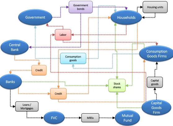
settings. Figure 1 provide an overview of the model, showing the main agents and their interactions through

markets. Arrows directions indicate the role that agents take in the markets, i.e. demand or supply.

Government bonds

Households

Consumption Goods Firms

Capital Goods Firm Government

Central Bank

Stock shares Labor

Consumption goods

Capital goods

Credit Credit

Banks

Loans / Mortgages

FVC MBSs Mutual_Fund

Housing units

Figure 1: Eurace model overview. Round boxes include agents, while rectangular boxes include markets. The outgoing arrows represent the supply and incoming arrows represents the demand

In the model agents’ decision processes are characterized by bounded rationality and limited capabilities

of computation and information gathering; thus, agents’ behavior follows adaptive rules derived from the

management literature about firms and banks, and from experimental economics literature about the behavior

4

See Fagiolo and Roventini (2017) for a survey and a comparison with DSGE models

5

of consumers and financial investors (Teglio et al., 2010; Raberto et al., 2012; Cincotti et al., 2012b; Teglio

et al., 2017). In general, agents interact in different types of markets, i.e. market for consumption goods and

capital good, housing market, labor market, credit market, securitisation market and financial market for

stocks and government bonds (figure 1). Most markets are based on a decentralized exchange with pairwise

trading, thus allowing us to capture some realistic features of goods, labour and credit markets, like price

dispersion, exchange out of equilibrium and rationing.

Furthermore, the balance sheet approach (Teglio et al., 2010) allows us to ensure the consistency at any

time step between stocks and flows in the model, both at the level of the single agent and at the aggregate

one, in line with the post-Keynesian stock-flow-consistent modeling approach (Godley and Lavoie, 2012).

Macroeconomic agent-based stock-flow constistent models have been developed up to date only in few works

(Kinsella et al., 2011; Riccetti et al., 2015; Caiani et al., 2016). In particular, Caiani et al. (2016) build a

general and flexible benchmark macroeconomic AB-SFC model, where the economy is fully decentralized and

all transactions between private agents occur through local interactions based on matching protocols. The

stock-flow consistency of a model allows to check that all monetary and real flows are accounted for, and

that all changes to stock variables are consistent with these flows6.

3. Novel modelling features

In this study, we aim to assess the systemic risk arising from the securitisation practise. For this purpose,

we enriched Eurace model with an improved securitisation process and a bank resolution mechanism, which

allows us to evaluate the risks for the whole economy entailed by banks’ bankruptcies. In the following, we

provide a description of the core modelling features related to this work, highlighting the new developments.

3.1. Securitisation process

The securitisation mechanism used in this paper is an enhancement of the one proposed in Mazzocchetti

et al. (2018). In particular, we have introduced an endogenous demand for mutual fund (MF) equity shares,

enabling the MF to finance its activity by issuing new shares, that can be purchased by households using part

of their monthly disposable income. This demand side specification plays a crucial role in the securitisation

functioning, since a restraint in MF liquidity hampers its capacity to purchase MBSs, thus forcing the banks

to retain unwanted credit in their balance sheet.

We recall here the main characteristics of the securitisation process, focusing on the mortgage case, and

then introduce the new features. The choice to securitise only mortgages relies on the opportunity to take

into account the prepayment risk, i.e. the risk that households pay off their mortgages through housing

units’ fire sales when financially distressed (a description of the housing market is recalled in the appendix,

6

for further details and related computational experiments with the housing market, see Ozel et al. (2016)).

The prepayment of mortgages plays a crucial role in the securitisation market, mainly for two reasons:

• Prepayments reduce the amount of mortgages in banks’ balance sheet; thus, a wave of mortgage

prepay-ments triggered by housing units’ fire sales may hamper banks’ possibilities to sell the desired amount

of mortgages to the FVC.

• Prepayments reduce the profits of banks and, if securitisation is active, also of the mutual fund. In

fact, whenever a mortgage is payed off the payments of its interest stops.

Securitisation mechanism allows banks to free up their balance sheet from mortgages and their related risk

by selling them to a Financial Vehicle Corporation (FVC), which finances its activity by creating

Mortgage-Backed Securities (MBSs) and selling them to a MF. Since Eurace includes a capital requirement provision

that mimics Basel II regulations, banks can exploit the securitisation process to reduce the risk weighted

assets in their balance sheet, thus complying with capital requirements without increasing their equity.

In the following, we describe the mortgage lending process and the securitisation framework. Let us

consider a bank bwith equityEb and risk-weighted portfolioWb, consisting of risk weighted loansWb,L and mortgagesWb,U, such that:

Wb =Wb,L+Wb,U. (1)

A householdhcan send a credit requests to banks. Whenever it enters in the housing market, it can buy

house units and, in case its liquidity is lower than the offered price, it asks for a mortgage. Let us assume

thatUbbhis the mortgage asked by the potential borrower (householdh) to the bankb. Bankbcan grant the

mortgage amount Ubbh to household honly if is endowed with an amount of equity which is higher than a

fraction of the risk-weighted assets in its balance sheet, i.e. it satisfies the capital requirement:

Eb>k(Wb+ωUbhUbbh) (2)

where k is fixed and equal to 0.17_{. Moreover, risk weight of household mortgages (ω} b

Uh) is assumed

constant and equal to 70%8_.

As stated in equation 2, bank’s lending activity is limited by the ratio of its risk-weighted assets and

equity. The ceiling of risk-weighted assets for the bank is given byαtimes its equity capital, i.e. αEb, where

α = 1_k. Thus, from a regulatory perspective, bank is constrained by the following rule: Wb ≤αEb. With

the introduction of the securitisation mechanism, the bank can put off its balance sheet the amount of

risk-weighted assets that exceed the ceiling; thus it could keep lending whenever Wb exceedsαEb. However, we

7

For a study of the effects of different capital requirements in Eurace see Raberto et al. (2012)

8

want to consider a behavioral specification that allows the bank to sell credit when it approaches the ceiling,

thus considering different thresholds, computed quarterly as a fraction of the ceiling. For this purpose, we

introduce an exogenous securitisation propensity parameter µ≤1. According toµ, the bank’s threshold is

given by (1−µ)αEb. The higher the value of µ, the lower will be the threshold of the bank, resulting in

more securitisation. In fact, whenever bank’s risk-weighted assets exceed the threshold, the bank computes

the amountSb of risk weighted assets that it want to sell to the FVC as:

Sb=Wb−(1−µ)αEb (3)

Conversely,Sbis set to zero (no securitisation), if bank’s risk-weighted assets do not exceed the threshold.

We define Ub as the amount mortgages in bank b balance sheet. It is worth remarking that Wb is the

sum of risk-weighted loans (Wb,L) and risk-weighted mortgages (Wb,U); thusSb is computed including also

the risk-weighted loans. However, we securitise only mortgages, which in extreme cases may be not enough

to fully satisfy the bank’s planned sales.

The amount of mortgages (USb) that the bank sell to the FVC is computed as the ratio betweenSb and

the bank’s risk-weighted mortgages and is uniformly distributed among bank’s mortgages. In particular:

(_U

Sb =

Sb

Wb,U

Ub if Wb,U > Sb

USb =Ub if Wb,U ≤Sb

(4)

FVC funds the purchase of loans and mortgages by issuing mortgage-backed securities (MBSs), that are

sold to the MF. In the same fashion of Mazzocchetti et al. (2018), the MF is endowed with an initial provision

of liquidity that allows it to purchase an amount of securitised products for two quarters, given a µ equal

to 100%. Furthermore, the fund aims at maintaining its liquidity at the target level (M∗

D), which represents

the amount of “operating liquidity” that is needed to carry out the securisation process for a quarter withµ

equal to 100%.

Each quarter, mutual fund computes its liquidity needsLD as:

(

LD=MD∗ −MD if MD∗ > MD

LD= 0 if M

∗

D≤MD

(5)

whereMD is the current liquidity of the fund. Therefore,LD represents the amount of liquidity that the

fund should rise. To do so the mututal fund can issue new equity shares, that generally are purchased by

households.

The rationale behind the use of a liquidity target relies on the choice to avoid a direct relation between

quarterly securitisation and the issuing of new shares, which would give rise to frequent shocks on households’

disposable income. On the contrary, a liquidity target let the fund to periodically adjust the liquidity level in

simply as a buffer for its securitisation activity, but relies on share issuing for financing new purchases.

The mutual fund computes quarterly the liquidity needed to reach its target, and, accordingly, issues new

shares that are bought by the households at the face value 9_{. Moreover, the mutual fund remunerates the}

owners of the issued shares paying a monthly interest, given by the central bank policy rate plus a spread

sD,t. To some extent the mutual fund may be considered as a fund whose benchmark is the policy rate,

which is outperformed by the spread sD,t. A minimum spread value ̟ is fixed, so that the mutual fund

always pays an interest that is higher than the policy rate. However, when new shares are to be issued, the

spread is increased by the mutual fund until it fulfills its liquidity needs. Accordingly, the spread is reduced

when the fund has enough liquid resources.

In order to link the spread to the fraction of disposable income that households are willing to invest

in equity shares, we enriched the behavioral specification of the demand side of mutual fund’s shares by

including the following relation:

bt=min(η sD,t, ̺) (6)

where bt is the fraction of disposable income that households use to purchase new shares,10 ̺ is the

maximum income percentage that households can invest andη is a parameter which represent the marginal

propensity of households’ investments in new shares with respect to the spread. In this setting,ηis equal to

15; thus for each yearly percentage point offered by the mutual fund as a spread on the policy rate, households

spend the 15 percent of their monthly disposable income to purchase the shares. Although the securitisation

is active on a quarterly base and the liquidity needsLD are updated accordingly with the same timing, the

issues of new shares occur monthly, in order to smooth the purchases across the quarters. The shares bought

by households give them the right to receive the earnings of the mutual fund, which are given by the interest

payments on the mortgages associated with securitised products.

It is worth remarking that the purchase of ABSs and MBSs by the mutual fund in the model is not

100% guaranteed. In particular, households are available to buy mutual fund’s shares only within a certain

proportion of their disposable income (̺); otherwise, mutual fund may not be able to finance the purchase

of ABSs and MBSs and securitisation stops until new funds are raised by the mutual fund.

3.2. Bailout

In order to tackle banks’ bankruptcies, we introduce a bailout mechanism which is activated whenever

the banks’ equity becomes negative.

It is worth remarking that, whenever credit rationing occurs, banks increase their equity by retaining

9

The face value is computed as the ratio between the nominal value of the mutual fund assets divided by the number of outstanding shares.

10

their earnings, with the aim to comply with the capital requirement (Wb ≤ αEb) and grant more credit.

However, bank’s equity may be reduced by loans and/or mortgages write-offs, which can occur in case of

GCPs bankruptcies or severe financial distress of households. If write-offs are high enough to make banks’

equity fall down below zero, the government intervenes by recapitalising the banks for an amount that allows

the credit institutions to re-comply with capital requirements.

Therefore, in this setting the cost of banks’ bankruptcies is supported by government and finally burden

the tax payers. In fact, the fiscal policy pursued by government is the stability and growth pact (SGP),

which targets a deficit to GDP raito of 3%. The bailout costs increase government spending and most likely

4. Computational experiments

Results are obtained by performing Monte Carlo computational experiments, i.e., simulations are run

using different seeds of the pseudorandom number generator for each scenario. Following Lauretta (2018)

and Mazzocchetti et al. (2018), we set five values of the securitisation propensityµ(0%, 5%, 10%, 20%, 30%).

Simulations have a duration of 35 years and are replicated using 50 different seeds per scenario, for a total

of 250 simulation runs. The computational experiments have been performed with the following settings:

3000 households, 50 Consumption Goods Producers, 3 Banks, 1 Capital Good Producer, 1 Financial Vehicle

Corporation, 1 Mutual Fund, 1 Government and 1 Central Bank.

Even though simulations run for a time span of 35 years, for the first five years banks are not allowed to

sell credit to the Financial Vehicle Corporation, thus there are five common years of transition phase, which

we do not consider in the analysis. Trajectories can diverge at the beginning of year 6, when banks can sell

mortgages to the FVC and the distinction among securitisation scenarios is enabled.

We present results using the median of yearly averages (computed across different time windows) over

the seeds for each one of the considered scenarios. In particular we show, for each of the five values of µ

(0%, 5%, 10%, 20%, 30%), the median of economic and financial variables over the 50 seeds, along with the

first and the third quartile. In the description of results, in-BS mortgages represent the mortgages accounted

in banks’ balance sheet, while off-BS mortgages are the mortgages securitised and put off banks’ balance

sheet. Total mortgages represent the sum of in-BS mortgages and off-BS mortgages. Furthermore, in order

to better distinguish between monetary and non-monetary variables, in the figures we use the symbol “Ee_”

(Eurace Euro) to refer to the currency unit in the model (see (see Ponta et al., 2018).

Moreover, to the aim of our investigation, we analyse a set of five indicators: banks’ leverage, i.e the ratio

between banks’ weighted assets and equity, computed using only in-BS weighted assets and total weighted

assets; mortgages to GDP ratio, computed using only in-BS mortgages and total mortgages; a fifth indicator,

the so-called VUC indicator (see Lauretta et al., 2016, and Eq. 7):

V U C=

PN

b=1T CT

Eqb

GDP (7)

This indicator can be seen as a transformation of the mortgage-to-GDP indicator in which the numerator

expresses the ratio between the sum of the portion of banks credits T CT forwarded to the securitisation

process (off-BS assets) and the total bank’s equity Eqb_{. Following the common practice in the literature}

(e.g. see Borio and Lowe, 2002a,b; Drehmann and Juselius, 2014), theGDP is used to scale the indicator.

The mortgage-to-GDP takes into account the leverage applied at the commercial bank level, but ignores the

role played by other leverages operating within the financial system at different levels. The VUC indicator

simply detects a second order of leverage, representative of the multi-leveraging effect operating within the

financial sector, which can trigger systemic financial risk. This indicator has a relevant obsevartory power

flows. For policy purposes, the VUC indicator used together with the most common mortgage-to-GDP ratio

can improve the early-warning detection of financial imbalancies in the financial system.

Finally, it is worth remarking that the indicators, differently from the other variables, are presented using

the median, the first and the third quartile of yearly values (computed only in certain years, i.e. year 1,

5, 10, 15, 20, 25, 30 after securitisation starts) over the seeds for each one of the five values ofµ (0%, 5%,

10%, 20%, 30%). The reason is given by the need to consider the yearly values of the indicators in order to

compute the cross-correlations. In fact, we present a cross-correlation analysis between the indicators and the

yearly number of bankruptcies. Moreover, we add a cross-correlation measure between mortgages-to-GDP

indicators and the yearly number of firesales. Therefore, in order to correctly perform the cross-correlations

analysis, we consider the yearly time series of the indicators.

5. Results

Results of the computational experiments show the economic impact of the securitisation process across

time, focusing on the effect on the housing market and, more in general, on a selection of relevant economic

variables. In the specific context of securitisation, we also introduce and test a set of systemic risk indicators,

that should be used as early warning for incoming financial crises.

In the next sections, we describe first the main economic implications of the securitisation process,

analysing the specific effect of different securitisation propensity (µ), and finally we examine the effectiveness

of the proposed risk indicators.

5.1. The securitisation mechanism

As outlined in section 3.1, the securitisation process involves banks, a financial vehicle corporation (FVC)

and a mututal fund (MF). The latter is provided with an intial amount of liquidity which covers two quarters

of securitisation with µ equal to 100%. Moreover, the MF targets a liquidity threshold, under which new

equity shares are issued and sold to households.

Figures 2 and 3 show the effects of the different scenarios on the MF. Scenarios with a higher value ofµ

show higher purchases of mortgage-backed securities (panel (b)) which are financed by means of both internal

resources and by issuing of new equity shares (panels (a) and (c)). However, households’ monthly income

percentage that can be invested in shares’ purchase is limited, thus an excess supply of MBSs may not be

sustained by the fund, and banks could be rationed, i.e. not able to fulfill their planned credit sales (panel

(d)).

Some details of the mutual fund equity shares are shown in figure 3. In particular, the mutual fund

pays an interest rate to reward shareholders (panel (a) shows the yearly interest rate paid by the fund), and

increases the spread whenever it needs to collect more liquidity, in order to attract more investors. This

happens more frequently in the case of high securitisation scenarios, as the liquidity needed by the fund to

their income in fund shares (panel (b)). It is worth remarking the interest rate of the MF shares is composed

by the CB policy rate (panel (c)) and a spread. According to the MF interest rate, the mutual fund pays

monthly dividends to the shareholders.

Figure 4 reports the main effects of the securitisation propensity on bank’s balance sheet. For higher

propensityµ, banks sell more mortgages, thus reducing the amount of mortgages accounted in banks’ balance

sheet (panel (b)) and enlarging the off-balance sheet volume (panel (a)). Consequently, the proportion of

off-BS mortgages over the total amount of credit enhances.

Securitisation allows banks to free up their balance sheet from risky assets, thus in the short run their

capital adequacy ratio increases and more credit can be granted by the bank. Therefore, the growth rate11_of

mortgages (which are securitised) is higher than the growth rate of firm’s loans (which are not securitised),

as shown in figure 6.

Those findings are in line with the securitisation mechanism explained in section 3.1. In particular,

according to equation 3, when securitisation is active banks de facto refer to their internal (adjusted) capital

adeguacy ratio (CAR), avoiding the regulatory constraints12_{. In particular, the securitisation instrument}

allows banks to escape the capital requirement obligation, by selling risk-weighted mortgages to the FVC in

exchange of liquidity. This aspect is highlighted in figure 10b, showing that bank leverage13 is much higher

in the case of securitisation.

5.2. Securitisation effects on credit and housing market

In order to assess the impact of securitisation on lending activity and on the housing market, we analyse

the total credit growth rate considering two different time horizons after the activation of the securitisation

mechanism: a short one presenting the first five years and a long one, where we report all the 30 years.

Panels (a), (b) and (c) of figure 5 show an increase in the volume of total credit in the first five years. In

fact, at the beginning of year 6 banks start to free up their balance sheets by selling risky assets, enabling

the issuing of additional credit. After one year, mortgages growth rates are higher in the scenarios with

positive µ, showing that securitisation accelerates credit growth. As the paper focuses on the securitisation

of mortgage loans, which means being able to expand the supply of mortgages, we set up a parametrization

of the housing market where the demand by households is also sustained14_{. This is the main reason why}

the mortgage loans growth rate is more affected by securitisation propensity with respect to the firms’ loans

growth rate.

The effect of securitisation in the medium and long run is shown in figure 6, and strictly depends on

securitisation propensity (µ). In fact, the higher the value ofµ, the lower are credit growth rates in the long

11

Growth rates are computed as the percentage increase of the selected indicatorI with respect to its value in year 5, when securitization is enabled, i.e.,g(t) = I(t)−_I(5)

/I(5)

12

in the current setting the capital requirement is fixed at 10%.

13

Bank leverage is the inverse of CAR, i.e., assets over equity. Here we refer to both in-BS and off-BS assets

14

In particular, the value of the stockTET Aand flowTDST I constraints is equal to 0.5, while probability to enter in the

housing market (ΦH) is 50%. For details on the effects of different parameterizations in the housing market see Ozel et al.

Mututal Fund data

1 5 10 15 20 25 30

years after securitization starts

0.5 1 1.5 2 2.5 3 10 5 0% 5% 10% 20% 30% (a)

1 5 10 15 20 25 30

years after securitization starts

0 0.5 1 1.5 2 2.5 3 10 5 0% 5% 10% 20% 30% (b)

1 5 10 15 20 25 30

years after securitization starts

0 2 4 6 8 10

N° of MF equity shares issued

104 0% 5% 10% 20% 30% (c)

1 5 10 15 20 25 30

years after securitization starts

0% 20% 40% 60%

securitisation rationing probability

0% 5% 10% 20% 30% (d)

Mutual fund shares issuing

1 5 10 15 20 25 30

years after securitization starts

0% 2% 4% 6% 8%

MF interest paid on issued shares

0% 5% 10% 20% 30% (a)

1 5 10 15 20 25 30

years after securitization starts

0 2% 4% 6% 8%

income % invested in MF shares

0% 5% 10% 20% 30% (b)

1 5 10 15 20 25 30

years after securitization starts

0% 1% 2% 3% 4% 5% 6% CB rate 0% 5% 10% 20% 30% (c)

1 5 10 15 20 25 30

years after securitization starts

0 50 100 150 200 250 300 0% 5% 10% 20% 30% (d)

Banks’ balance sheet data

1 5 10 15 20 25 30

years after securitization starts

0 0.5 1 1.5 2 2.5 3 10 5 0% 5% 10% 20% 30% (a)

1 5 10 15 20 25 30

years after securitization starts

0 1 2 3 4 5 10 5 0% 5% 10% 20% 30% (b)

1 5 10 15 20 25 30

years after securitization starts

0% 20% 40% 60%

off-BS mortgages / total credit

0% 5% 10% 20% 30% (c)

1 5 10 15 20 25 30

years after securitization starts

0.5 1 1.5 2 2.5 3 3.5 10 4 0% 5% 10% 20% 30% (d)

run. This is mainly due to the higher instability triggered by the short-term boost of lending activity, not

supported by an adeguate equity base increase, but built only on mortgages sales. In fact, securitisation may

be impaired because the mutual fund does not have enough funds (panel (d) of figure 2) and whenµis high

banks may find it difficult to increase their equity base by retaining earnings, since most of them flow out to

off-BS mortgages. The results can be an increase in credit rationing (panel (a) of figure 7) and a decrease

of loans and mortgages growth rate. Moreover, in the long run a low equity level increases the risk of banks

bankruptcies due to credit write-offs.

The dynamics of the housing market is strictly linked with the mortgage volumes. In fact, the easier access

to mortgage loans enhances the demand for housing units by households, triggering a boost in the housing

price (panel (b) of figures 5 and 6). Following the dynamics of the mortgages, the housing unit price growth

rate is larger in the short run (after securitisation has been enabled) and for higher values of securitisation

propensity. However, in the medium and long run results may be reversed, with scenarios characterized by

greaterµshowing a slow down of the housing market activity, culminating in higher fire-sales volumes (figure

6e).

It is worth noting that both in the credit and housing markets a low value of securitisation propensity

(µ= 5%) achieves the best results, boosting credit activity in the short run without suffering growth rate

decreases in the long run with respect to the baseline scenario (µ= 0%).

5.3. Securitisation impact on firms

The effects of securitisation process affect also the financing activity of firms. In particular, following the

pecking order theory, Consumption Goods Producers (CGPs) first finance their production plan by means

of internal resources, then they resort to bank credit, and finally, if rationed in the credit market, they issue

new shares and sell them to households.

Thus, a boost or a restraint in banks’ lending activity changes the financial structure of GCPs. In fact,

as the securitisation process starts and banks are able to free up their balance sheet from risky assets, thus

improving their capability to grant new loans to firms, CGPs face lower rationing in the credit market. Panel

(a) of figure 7 illustrates this aspect, showing a reduction of credit rationing in the very first year after

securitisation starts. However, in scenarios where the propensity µis high, the lower bank equity level and

the increase of fire-sales (figure 6e) that reduces the amount of mortgages in banks’ balance sheet, may impair

the securitisation process (see section 3.1) and increase the number of credit rationing in the medium and

long run.

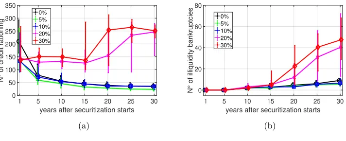
The higher frequency of firms rationed in the credit market leads to a higher number of illiquidity

bankruptcies, where firms are no more able to roll over debt and finance their production plan (figure 7b).

5.4. Securitisation effects on government accounting

Figure 8 shows the impact that banks’ defaults have on the government accounting. As stated in section

Growth rates

1 2 3 4 5

years after securitization starts

12% 14% 16% 18% 20%

total mortgages growth rate

0% 5% 10% 20% 30% (a)

1 2 3 4 5

years after securitization starts

6% 8% 10% 12% 14% 16% 18% 20%

housing price growth rate

0% 5% 10% 20% 30% (b)

1 2 3 4 5

years after securitization starts

8% 10% 12% 14% 16% 18% 20%

loans growth rate

0% 5% 10% 20% 30% (c)

1 2 3 4 5

years after securitization starts

10% 12% 14% 16% 18% 20%

total credit growth rate

0% 5% 10% 20% 30% (d)

Growth rates

1 5 10 15 20 25 30

years after securitization starts

0% 5% 10% 15% 20% 25% 30%

total mortgages growth rate

0% 5% 10% 20% 30% (a)

1 5 10 15 20 25 30

years after securitization starts

0% 5% 10% 15% 20% 25% 30%

housing price growth rate

0% 5% 10% 20% 30% (b)

1 5 10 15 20 25 30

years after securitization starts

0% 5% 10%

loans growth rate

0% 5% 10% 20% 30% (c)

1 5 10 15 20 25 30

years after securitization starts

-5% 0% 5% 10% 15%

total credit growth rate

0% 5% 10% 20% 30% (d)

1 3 5 10 15 20 25 30

years after securitization starts

0% 2% 4% 6% 8% 10% 12%

firesales / HM volume

0% 5% 10% 20% 30% (e)

Firms’ data

1 5 10 15 20 25 30

years after securitization starts

0 50 100 150 200 250 300 350

N° of credit rationing

0% 5% 10% 20% 30%

(a)

1 5 10 15 20 25 30

years after securitization starts

0 20 40 60 80

N° of illiquidity bankruptcies

0% 5% 10% 20% 30%

(b)

Figure 7: Yearly mean’s median, first quartile and third quartile over 50 seeds of a set of firms’ data. Yearly means are computed across different time windows, each of them reported in the x-axis. Five securitisation propensity values (µ) are considered (0%,5%,10%,20%,30%)

negative, the government provides the banks with the liquidity necessary to exceed the regulatory capital

requirement and carry on lending activity. However, bailout costs are paid by the government (panel (c) in

figure 8), increasing its expenses (panel (a) in figure 8) and deficit to GDP ratio (panel (b) in figure 8). In a

Stability and growth pact scenario15_{, this leads to an increase of taxes, de facto offloading the costs of bailout}

on taxpayers (panel (d) in figure 8).

5.5. Securitisation and macroeconomic variables

By affecting the credit and the housing market, securitisation also impacts the main macroeconomic

indicators. Figure 9 shows real consumption (panel (a)) and unemployment rate (panel (b)). In the short

and medium run the securitisation process allows banks to grant more credit (figures 5), triggering also an

expansionary effect on consumption (in relative terms, comparing the different values ofµ) and a consequent

reduction of the unemployment rate. However, in the longer run, expecially for scenarios with µ = 20%

and 30%, the higher instability of the banking system, subsidized by taxpayers by means of recessive fiscal

policies, leads to higher levels of unemployment.

5.6. Systemic risks indicators

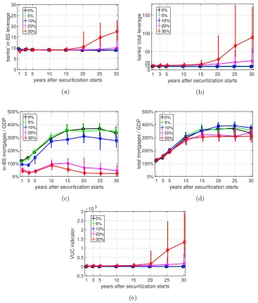
Figure 10 presents the time evolution of five systemic risk indicators, which are potential candidates to

be used as early warnings for incoming financial crises. As the focus of the paper is on the banking system

and credit market, we examined indicators that mainly target banks’ assets. In particular, we distinguish

two types of indicators, a first one, reported in figures 10a and 10c, which considers only assets in the balance

sheet of the bank, and a second one, reported in figures 10b, 10d and 10e, which includes also off-balance

sheet assets.

15

Government data

1 5 10 15 20 25 30

years after securitization starts

25% 30% 35% 40% 45% 50% 55%

government expenses / GDP

0% 5% 10% 20% 30% (a)

1 5 10 15 20 25 30

years after securitization starts

-5% 0% 5% 10% 15% 20% 25%

deficit / GDP

0% 5% 10% 20% 30% (b)

1 5 10 15 20 25 30

years after securitization starts

0% 5% 10% 15%

bailout costs / GDP

0% 5% 10% 20% 30% (c)

1 5 10 15 20 25 30

years after securitization starts

15% 20% 25% 30% 35% tax rate 0% 5% 10% 20% 30% (d)

Figure 8: Yearly mean’s median, first quartile and third quartile over 50 seeds of a set of government data. Yearly means are computed across different time windows, each of them reported in the x-axis. Five securitisation propensity values (µ) are considered (0%,5%,10%,20%,30%)

Macroeconomic data

1 5 10 15 20 25 30

years after securitization starts

1.1 1.2 1.3 1.4 1.5 1.6 1.7 1.8 real consumption 105 0% 5% 10% 20% 30% (a)

1 5 10 15 20 25 30

years after securitization starts

0% 5% 10% 15% 20% 25% unemployment rate 0% 5% 10% 20% 30% (b)

The indicators in the upper row (figures 10a and 10b) represent bank leverage, computed as the ratio

between bank’s weighted assets and equity. The indicators in the middle row (figures 10c and 10d) focus

on the ratio between mortgages and GDP, while the last indicator (figure 10e) focuses specifically on the

off-balance sheet assets, as explained in section 4.

We remind here that the capital requirements for banks are set to 10%, therefore allowing for a maximum

leverage of 10. Indeed, banks are able to comply with a leverage value under 10 until year 15, as figure 10a

shows, while afterwards the leverage tends to increase in the case of higher securitization propensity, as banks

are not stockpiling enough capital buffer. The leverage measure increases when also off-balance assets are

considered, as in figure 10b, supposedly revealing a higher systemic risk in the economy.

In a similar way, figure 10d shows the mortages to GDP ratio when also off-balance mortgages are

considered. However, in this case, differently from the previous one, the risk indicator in the high securitisation

scenarios are lower. Therefore this indicator does not warn about a higher risk when securitisation is active.

The last indicator, in figure 10e, which targets directly the off-balance sheets assets, weighted by the

economic activity (GDP), reveals, on the other hand, a strong risk in the case of high securitisation scenarios.

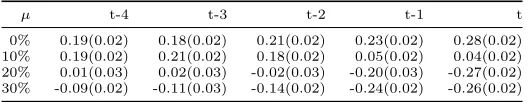
We assess the effectiveness of the different risk indicators in predicting economic and financial crises by

examining the cross-correlation of the indicators with the number of total bankruptcies, used as a proxy for

the crisis. Tables from 1 to 5 report these cross-correlations, considered with negative lags up to four years,

even if we are mainly interested to examine the minus one lag, i.e., the correlation of total bankruptcies with

the risk indicator one year before.

In principle, a good indicator should have a high correlation value for all the different scenarios, as the

securitisation propensity is not directly observable in the real world. In general, indicators including off-BS

assets have a better performance, while the ones excluding them could be completely misleading as in the

case of table 3, where the cross-correlation at t−1 is even negative. In particular, the total mortgage to

GDP indicator and the VUC indicator show both a positive and consistent correlation between the number

of bankruptcies and the value of the indicators in the previous years. However, the values of the correlation

coefficients are not extremely high and it is not easy to identify a clear “alarm” threshold, beyond which the

economy should be considered at danger.

In tables 6 and 7 we use fire-sales in the housing market as an alternative indicator for measuring the

magnitude of the crisis. Results show again that it is essential to consider indicators with off-BS assets

in the high securitisation scenarios. Moreover the correlation between the mortgage to GDP indicator with

successive crises (measured as fire-sales amount) is stronger. This can be explained by the fact that borrowers

of mortgage loans are the first “victims” of an extra leveraged credit market, and therefore the effect on

fire-sales is stronger. The effect on firms’ bankruptcies is still there, but it is attenuated by a longer economic

Systemic risk indicators

1 3 5 10 15 20 25 30

years after securitization starts

0 5 10 15 20 25 30

banks' in-BS leverage

0% 5% 10% 20% 30% (a)

1 3 5 10 15 20 25 30

years after securitization starts

0 10 20 50 100 150

banks' total leverage

0% 5% 10% 20% 30% (b)

1 3 5 10 15 20 25 30

years after securitization starts

0% 100% 200% 300% 400% 500%

in-BS mortgages / GDP

0% 5% 10% 20% 30% (c)

1 3 5 10 15 20 25 30

years after securitization starts

0% 100% 200% 300% 400% 500%

total mortgages / GDP

0% 5% 10% 20% 30% (d)

1 3 5 10 15 20 25 30

years after securitization starts

-0.5 0 0.5 1 1.5 2 2.5 3 VUC indicator 10-3 0% 5% 10% 20% 30% (e)

Crosscorrelations

µ t-4 t-3 t-2 t-1 t

0% -0.07(0.01) -0.20(0.02) -0.31(0.02) -0.06(0.02) 0.28(0.01) 10% -0.04(0.01) -0.08(0.01) -0.10(0.01) 0.01(0.01) 0.26(0.01) 20% 0.13(0.03) 0.14(0.04) 0.12(0.04) 0.19(0.03) 0.28(0.03) 30% 0.23(0.04) 0.25(0.04) 0.22(0.04) 0.22(0.04) 0.19(0.03)

Table 1: Cross-correlation of regulatory leverage (banks’ equity to in-BS weighted assets ratio) and total bankruptcies. Standard errors in parentheses

µ t-4 t-3 t-2 t-1 t

0% -0.07(0.01) -0.20(0.02) -0.31(0.02) -0.06(0.02) 0.28(0.01) 10% -0.05(0.01) -0.08(0.01) -0.05(0.01) 0.21(0.01) 0.40(0.02) 20% 0.23(0.03) 0.26(0.03) 0.27(0.04) 0.34(0.03) 0.35(0.03) 30% 0.33(0.03) 0.36(0.04) 0.31(0.03) 0.29(0.03) 0.18(0.03)

Table 2: Cross-correlation of total leverage (banks’ equity to total weighted assets ratio) and total bankruptcies. Standard errors in parentheses

µ t-4 t-3 t-2 t-1 t

0% 0.19(0.02) 0.18(0.02) 0.21(0.02) 0.23(0.02) 0.28(0.02) 10% 0.19(0.02) 0.21(0.02) 0.18(0.02) 0.05(0.02) 0.04(0.02) 20% 0.01(0.03) 0.02(0.03) -0.02(0.03) -0.20(0.03) -0.27(0.02) 30% -0.09(0.02) -0.11(0.03) -0.14(0.02) -0.24(0.02) -0.26(0.02)

Table 3: Cross-correlation of in-BS mortgages to GDP ratio and total bankruptcies. Standard errors in parentheses

µ t-4 t-3 t-2 t-1 t

0% 0.19(0.02) 0.18(0.02) 0.21(0.02) 0.23(0.02) 0.28(0.02) 10% 0.14(0.01) 0.17(0.02) 0.17(0.02) 0.19(0.02) 0.24(0.02) 20% 0.15(0.02) 0.18(0.02) 0.19(0.02) 0.23(0.02) 0.25(0.02) 30% 0.16(0.01) 0.18(0.01) 0.18(0.02) 0.24(0.02) 0.27(0.02)

Table 4: Cross-correlation of total mortgages to GDP ratio and total bankruptcies. Standard errors in parentheses

µ t-4 t-3 t-2 t-1 t

0%

10% -0.08(0.02) -0.07(0.02) 0.03(0.02) 0.43(0.02) 0.48(0.02) 20% 0.24(0.03) 0.26(0.03) 0.26(0.03) 0.35(0.03) 0.30(0.03) 30% 0.27(0.03) 0.28(0.03) 0.22(0.03) 0.22(0.03) 0.12(0.03)

Table 5: Cross-correlation of VUC indicator and total bankruptcies. Standard errors in parentheses

µ t-4 t-3 t-2 t-1 t

0% 0.23(0.02) 0.27(0.01) 0.41(0.01) 0.47(0.01) 0.60(0.01) 10% 0.23(0.02) 0.25(0.02) 0.34(0.02) 0.36(0.01) 0.51(0.01) 20% 0.07(0.03) 0.07(0.03) 0.13(0.03) 0.05(0.03) 0.09(0.03) 30% -0.06(0.02) -0.07(0.02) -0.03(0.02) -0.08(0.02) 0.01(0.03)

µ t-4 t-3 t-2 t-1 t 0% 0.23(0.01) 0.27(0.01) 0.41(0.01) 0.47(0.01) 0.60(0.01) 10% 0.26(0.01) 0.30(0.01) 0.42(0.01) 0.43(0.01) 0.59(0.01) 20% 0.24(0.01) 0.24(0.01) 0.38(0.01) 0.27(0.01) 0.51(0.01) 30% 0.24(0.01) 0.23(0.01) 0.37(0.01) 0.26(0.01) 0.47(0.01)

6. Conclusions

The paper studies the effects of the securitisation process in the assessment of systemic financial risk

indicators, using the agent-based model Eurace, which includes a housing market in the style of Ozel et al.

(2016), and implements a securitisation mechanism on the footprints of Mazzocchetti et al. (2018) and

Lauretta (2018) that allows banks to free up their balance sheets from risk-weighted assets and circumvent

the prudential capital requirements. The model has been enriched with an endogenous demand specification

of mutual fund equity shares and with a bailout resolution mechanism, which foresees the banks’ rescue by

means of government spending if banks’ equity becomes negative.

We analyse the impact of securitisation on credit market and on real economy, finding that scenarions

with higher securitisation propensities weaken the financial stability of banks with relevant effects on different

sectors of the economy. Moreover, a set of five systemic financial risk indicators is considered: banks’ leverage,

i.e the ratio between banks’ weighted assets and equity, computed using only in-BS weighted assets and total

weighted assets; mortgage to GDP ratio, computed using only in-BS mortgages and total mortgages; a fifth

indicator, the so-called VUC indicator, which is given by the ratio between off-balance sheet credit and banks’

equity, normalized with the GDP.

The results presented in the paper brings clear evidence of the role played by the securitisation process,

above certain levels of securitisation propensity, in paving the way toward booms and busts and ensuing

economic recessions. Furthermore, the analysis shows how banks can satisfy their capital requirements while

contributing to gradually building up higher risk exposure of the whole financial system.

The outcome of the computational experiments show that while the mortgage-to-GDP and banks’ leverage

can be misleading when considering only in-BS assets, thus not detecting correctly the financial imbalances,

the adjusted version of those indicators together with the VUC indicator instead seem more adequate to

monitor and anticipate this risk exposure.

Therefore, the paper highlights the importance of considering off-BS items when assessing for systemic

risk. However, we remain of the opinion that this does not mean to downgrade the systemic risk indicators

based on in-BS items, but their analysis and interpretation for regulatory reasons should be integrated

the off-BS items, which play a relevant role in detecting systemic risk, as our results shows. The ABM

framework allows to analyse, through numerical simulations, the relevance of off-balance assets in assessing

systemic financial risk. Otherwise, this would be more complicated to verify empirically, given the lack of

data availability on banks’ off-BS assets. Only recently, the European Central Bank has started to gather

from the Special Purpose Vehicle/Entity (SPV/SPE) these kind of data for the Euro area.

The data are available from 2012 annually and only from 2014 are they provided quarterly. Future work

needs to be done in this direction, and our analysis contributes to highlight as a priority for regulation the

access to the off-BS assets data. Of course, other variables can play an important role in developing systemic

risk, such as, among others, the size of financial institutions and the exposure in interbank lending. Future

in-BS and off-BS dimensions, but incorporate also other possible relevant variables for monitoirng systemic

Acknowledgment

The authors acknowledge EU-FP7 collaborative project SYMPHONY16 _{under grant no. 611875.}

16

References

Acharya, V. V., Pedersen, L. H., Philippon, T., Richardson, M., 2017. Measuring systemic risk. The Review

of Financial Studies 30 (1), 2–47.

Adrian, T., Brunnermeier, M. K., 2016. Covar. American Economic Review 106 (7), 1705–1741.

Bandt, O., Hartmann, P., Peydr´o, J., 2012. Systemic Risk in Banking: An Update. Oxford University Press,

Oxford.

Banulescu, G., Dumitrescu, E., 2015. Which are the SIFIs? a component expected shortfall approach to

systemic risk. Journal of Banking and Finance 50, 575–588.

Barrell, R., Davis, E., Karim, D., Liadze, I., 2010. Bank regulation, property prices and early warning systems

for banking crises in OECD countries. Journal of Banking & Finance 34, 2255–2264.

Billio, M., Getmansky, M., Lo, A., Pelizzon, L., 2012. Econometric measures of connectedness and systemic

risk in the finance and insurance sectors. Journal of Financial Economics 104 (3), 535–559.

BIS, 2017. High-level summary of basel III reforms. Basel Committee on Banking Supervision.

Borio, C., Lowe, P., 2002a. Asset prices, financial and monetary stability: Exploring the nexus. BIS Working

Papers 114, Bank for International Settlements.

Borio, C., Lowe, P., 2002b. Securing sustainable price stability: Should credit come back from the wilderness?

BIS Working Papers 157, Bank for International Settlements.

Brunnermeier, M. K., Sannikov, Y., 2014. A macroeconomic model with a financial sector. American

Eco-nomic Review 104 (2), 379–421.

Caiani, A., Godin, A., Caverzasi, E., Gallegati, M., Kinsella, S., Stiglitz, J. E., 2016. Agent based-stock flow

consistent macroeconomics: Towards a benchmark model. Journal of Economic Dynamics and Control 69,

375–408.

Cappiello, L., Kadareja, A., Kok, C., Protopapa, M., 2010. Do bank loans and credit standards have an effect

on output? A panel approach for the euro area. Working Paper Series 1150, European Central Bank.

Cincotti, S., Raberto, M., Teglio, A., 2010. Credit money and macroeconomic instability in the agent-based

model and simulator Eurace. Economics - The Open-Access, Open-Assessment E-Journal 4, 1–32.

Cincotti, S., Raberto, M., Teglio, A., 2012a. The Eurace macroeconomic model and simulator. In:

Agent-based Dynamics, Norms, and Corporate Governance. The proceedings of the 16-th World Congress of the

Cincotti, S., Raberto, M., Teglio, A., 2012b. Macroprudential policies in an agent-based artificial economy.

Revue de l’OFCE 124 (5), 205–234.

Dawid, H., Gemkow, S., Harting, P., van der Hoog, S., Neugart, M., 2018. Agent-Based Macroeconomic

Modeling and Policy Analysis: The Eurace@Unibi Model. Oxford University Press, pp. 490–519.

Deghi, A., Welz, P., ˙Zochowski, D., 2018. A new financial stability risk index to predict the near-term risk

of recession. Financial Stability Review.

Delli Gatti, D., Desiderio, S., 2015. Monetary policy experiments in an agent-based model with financial

frictions. Journal of Economic Interaction and Coordination 10 (2), 265–286.

Diebold, F., Yilmaz, K., 2014. On the network topology of variance decompositions: measuring the

connect-edness of financial firms. Journal of Econometrics 182 (1), 119–134.

Dosi, G., Napoletano, M., Roventini, A., Treibich, T., 2017. Micro and macro policies in the

Keynes+Schumpeter evolutionary models. Journal of Evolutionary Economics 27 (1), 63–90.

Drehmann, M., Juselius, M., 2014. Evaluating early warning indicators of banking crises: satisfying policy

requirements. International Journal of Forecasting 30 (3), 759–780.

ECB, 2009. The concept of systemic risk. Financial Stability Review.

ECB, 2011. Systemic risk methodologies. Financial Stability Review.

Fagiolo, G., Roventini, A., 2017. Macroeconomic policy in DSGE and agent-based models redux: new

devel-opments and challenges ahead. Journal of Artificial Societies and Social Simulation, 20 (1), 1.

Gerhardt, M., Vennet, R. V., 2017. Bank bailouts in Europe and bank performance. Finance Research Letters

22, 74–80.

Godley, W., Lavoie, M., 2012. Monetary Economics: An Integrated Approach to Credit, Money, Income,

Production and Wealth, 2nd Edition. Palgrave Macmillan: Basingstoke.

Goodhart, C., Segoviano, M., 2009. Banking stability measures. FMG discussion papers, Financial Markets

Group.

Gray, D. F., Merton, R. C., Bodie, Z., 2008. New framework for measuring and managing macrofinancial risk

and financial stability. Harvard Business School Working Paper 09-015, Levy Economics Institute.

Guerini, M., Lamperti, F., Mazzocchetti, A., 2018. Unconventional monetary policy: between the past and

future of monetary economics. European Journal of Economics and Economic Policies 15 (2), 122 – 131.

Huang, X., Zhou, H., Zhu, H., 2009. A framework for assessing the systemic risk of major financial institutions.

Huang, X., Zhou, H., Zhu, H., 2012. Systemic risk contributions. Journal of Financial Services Research

42 (1), 55–83.

Kinsella, S., Greiff, M., Nell, E. J., 2011. Income distribution in a stock-flow consistent model with education

and technological change. Eastern Economic Journal, 37 (1), 134–149.

Lauretta, E., 2018. The hidden soul of financial innovation: An agent-based modelling of home mortgage

securitization and the finance-growth nexus. Economic Modelling, 68, 51–73.

Lauretta, E., Chaudhry, S. M., Mullineux, A. W., 2016. Theory and evidence on the finance-growth

relation-ship: The virtuous and unvirtuous cycles. Discussion Paper 2016-8, University of Birmingham, Financial

Resilience Research Cluster.

Lehar, A., 2005. Measuring systemic risk: A risk management approach. Journal of Banking & Finance

29 (10), 2577–2603.

Mazzocchetti, A., Raberto, M., Teglio, A., Cincotti, S., 2018. Securitisation and business cycle: An

agent-based perspective. Industrial and Corporate Change (in press).

Misina, M., Tkacz, G., 2009. Credit, asset prices, and financial stress. International Journal of Central

Banking, 5 (4), 95–122.

Napoletano, M., Roventini, A., Sapio, S., 2006. Are business cycles all alike? A bandpass filter analysis of

the italian and US cycles. Rivista italiana degli economisti, 1/2006, 87–118.

Ozel, B., Nathanael, R. C., Raberto, M., Teglio, A., Cincotti, S., 2016. Macroeconomic implications of

mortgage loans requirements: an agent based approach. Working Papers 2016/05, Economics Department,

Universitat Jaume I, Castell´on (Spain).

Petrovic, M., Ozel, B., Teglio, A., Raberto, M., Cincotti, S., 2017. Eurace open: An agent-based multi-country

model. Working Papers 2017/09, Economics Department, Universitat Jaume I, Castell´on (Spain).

Ponta, L., Raberto, M., Teglio, A., Cincotti, S., 2018. An agent-based stock-flow consistent model of the

sustainable transition in the energy sector. Ecological Economics 145, 274–300.

Raberto, M., Teglio, A., Cincotti, S., 2012. Debt deleveraging and business cycles. an agent-based

persperc-tive. The Open-Access, Open-Assessment E-Journal, 6, 2012–27.

Riccetti, L., Russo, A., Gallegati, M., 2015. An agent based decentralized matching macroeconomic model.

Journal of Economic Interaction and Coordination, 10 (2), 305–332.

Schwaab, B., Koopman, S. J., Lucas, A., 2011. Systemic risk diagnostics: coincident indicators and early

Teglio, A., Mazzocchetti, A., Ponta, L., Raberto, M., Cincotti, S., 2017. Budgetary rigour with stimulus in

lean times: Policy advices from an agent-based model. Journal of Economic Behavior and Organization

(in press).

Teglio, A., Raberto, M., Cincotti, S., 2010. Balance sheet approach to agent-based computational economics:

The Eurace project. In: Combining Soft Computing and Statistical Methods in Data Analysis. Vol. 77 of

Advances in Intelligent and Soft Computing. Springer Berlin / Heidelberg, pp. 603–610.

Trichet, J., 2009. Clare distinguished lecture in economics and public policy. University of Cambridge, 10

December 2009.

Uribe, M., Schmitt-Groh´e, S., 2017. Open economy macroeconomics. Princeton University Press: Princeton,

New Jersey.

Watson, M., Stock, J., 1999. Business Cycle Fluctuations in U.S. Macroeconomic Time Series. Elsevier,