Munich Personal RePEc Archive
World Equalized Factor Price and
Integrated World Trade Space
Guo, Baoping
Individual Researcher
September 2018
Online at
https://mpra.ub.uni-muenchen.de/92503/
1
World Equalized Factor Price and Integrated World Trade Space
Baoping Guo1
Abstract – This study derived a general equilibrium for the Heckscher-Ohlin model at the
context of higher dimensions. The equalized factor price at the equilibrium is the Dixit-Norman price, i.e. that the world price will remain the same when allocations of factor
endowments change within the IWE box2. The study explored a way to show the legacy of
comparative advantages on the Heckscher-Ohlin model and demonstrated that the equalized factor price and world commodity price at the equilibrium ensured that the countries participating free trade gain from trade. The solution analytically addresses the Heckscher-Ohlin theorem with trade volume, the Factor-Price Equalization theorem with price solution, and comparative advantages with gains from trade. It shows the hided important logic in the IWE and the Heckscher-Ohlin model as that world factor endowments determine world price.
Keyword: Factor Price Equalization, Factor Price Localization, Heckscher-Ohlin Model,
General Equilibrium, Cone of Commodity Price, Cone of Diversification.
JEL Classification: F11
1. Introduction
The world trade equilibrium is an important field of general equilibrium theory. Its task is just as Lionel McKenzie (1987) described,
“Walras set of major objectives of general equilibrium theory as they have remained
ever since. First, it was necessary to prove in any model of general equilibrium that the equilibrium exists. Then its optimality properties should be demonstrated. Next, it should be shown how the equilibrium would be attained, that is, the stability of the equilibrium and its uniqueness should be studied. Finally, it should be shown how the equilibrium will change when conditions of demand, technology, or resources are varied.”
The Heckscher-Ohlin model is attractive, due to its capacities to show general trade equilibriums of multiple commodities, made by different factors, and trade by many countries from the model structure. Paul Samuelson and Lionel McKenzie are pioneers
both in general equilibrium theory and in international trade theory.Dixit and Norman
(1980) and Woodland (1982) build a foundation of the dual approach to study trade
1 Former faculty member of The College of West Virginia (CWV is renamed as Mountain State University, now it is the Beckley campus of West Virginia University), corresponding address: 8916 Garden Stone Lane, Fairfax, VA 22031, USA. Email address: bxguo@yahoo.com.
2
2
equilibrium. The factor-price equalization is the major focus for the studies of general trade
equilibriums of the Heckscher-Ohlin model. Dixit and Norman (1980)’s integrated world
equilibrium (IWE) is a so important contribution to understanding trade equilibriums and the FPE both from the supply side and from the demand side. Deardorff(1994) mentioned that the IWE is “Perhaps the most useful and enlightening approach to FPE”. Dixit and Norman (1980) demonstrated that the IWE box boarded by the cone of diversification
shares one equalized factor price (and commodity price). It described a “dynamic” and
mobile characteristic of general equilibrium. It paves the way to find what the equalized factor price is. It actually sets up a reference standard to evaluate if an equilibrium price is suitable to the Heckscher-Ohlin model. Helpman and Krugman (1985) popularized the IWE approach for the equilibrium analyses. Wu (1987) and Deardroff (1994) studied the FPE by the approach of the IWE on higher dimensions. Dearroff (1994) identified the lenses within the IWE for the FPE under multiple commodities.
The general equilibrium is a market process. The free trade tends to optimize distribution of
goods and services in at least some ways. A country participated in trade tends maximizing its welfare by minimizing its trade-off. A proper utility function to reflecting trade gaming
properties is useful to attain a general equilibrium of commodity, factor, and multi-country economy.
Guo (2018) provided a general equilibrium of trade for the 2 x 2 x 2 model. The equalized price at the equilibrium is just the price Dixit-Norman predicted. This is a very useful theoretical result, which shows the legacy of the model structure of the Heckscher-Ohlin theories.
Along the long tradition of researches in the general equilibrium of trade and the FPE, this study derives a general equilibrium of trade for higher dimensions model by using the IWE approach. The higher dimensions here are arbitrary factors, arbitrary commodities, and arbitrary countries. The FTE price at the equilibrium of this paper is the Dixit-Norman price; it allows mobile factors across countries without shifting the FPE.
The major concern of this paper is about conditions for the solution of general equilibrium in higher dimension. From the analysis view or methodology, the study finds that the country number is not an issue for the general equilibrium with higher dimensions model. We can address this issue by answer question that who is the trade partners for a country in multiple-country models. The trade partner for a country is the rest of the world. By this understanding, the analyses will be very simple; it is just like the analyses for the two-country economy, a two-country vs the rest of the world. The key point here is that the world price should reach the same results by analyses of the different country vs its rest of world.
3
Moreover, the factor number somehow is an issue when it is greater than 2, assuming that we process equilibrium analyses from factor contents of trade. The trade balance is a critical condition for trade equilibrium analysis. However, it is only a single equation, no matter how many factors were involved. For two-factor case, it just is the term of trade or the term of factor content of trade. We can obtain a relative factor price or relative
commodity price. For higher dimensions (N>=3), the trade balance is with multiple factor variables in one single equation, we cannot get a relative price for any pair of factors. For N=3, we miss one condition for the solution of equilibrium, For N=4, we miss two
conditions. For N=n, we miss N-2 conditions. This means that the equilibrium solution is not determined from the mathematical view. The budget condition is another format of
trade balance condition3, which is used in most equilibrium analysis. This is a challenge to
analyze general equilibrium. We did not explore this issue before. This issue not only challenges this study but also challenges other studies in this field. Using a utility function may solve fewer variables if it is properly designed. We provide a solution to this issue in this study.
This paper is divided into 6 sections. Section 2 reviews the trade equilibrium for the 2x2x2 model. Section 3 investigates the general equilibrium of trade of the 3x3x3 model in detail. Section 4 provides the general world trade equilibrium for multiple factors, multiple commodities, and multiple countries (the N x M x Q model). Section 5 studies the gains from trade by using prices at the equilibrium. Section 6 is discussions for the equilibriums.
2. Review of the general equilibrium of the 2 x 2 x 2 model
With the normal assumptions of the Heckscher-Ohlin theory, a standard 2 x 2 x 2 model can be presented as the following:
a. The production constraint of full employment of resources are
𝐴𝑋ℎ = 𝑉ℎ (ℎ = 𝐻, 𝐹) (2-1)
where A is a 2x2 technology matrix, Xh is a 2 x1 vector of commodities of country h, Vh a
2x1 vector of factor endowments of country h. The elements of matrix A is 𝑎𝑘𝑖(𝑊), 𝑘 =
𝐾, 𝐿, 𝑖 = 1,2.
b. The zero-profit unit cost condition
𝐴′𝑊∗ = 𝑃∗ (2-2)
where 𝑊∗is a 2 x1 vector of factor prices, P∗ is a 2x1 vector of commodity prices. Both 𝑃∗
and 𝑊∗ are world price when factor price equalization reached.
c. The definition of the share of GNP of country h to world GNP,
𝑠ℎ = 𝑃′ 𝑋ℎ/𝑃′ 𝑋𝑊 (ℎ = 𝐻, 𝐹) (2-3)
d. The trade balance condition is
𝑃′ 𝑇ℎ = 0 (ℎ = 𝐻, 𝐹) (2-4)
or
𝑊′ 𝑉ℎ = 0 (ℎ = 𝐻, 𝐹) (2-5)
e. The constraint of the cone of diversification of factor endowments
3 Budget condition is dependent on trade balance condition
4
𝑎𝐾1 𝑎𝐿1 >
𝐾𝐻
𝐿𝐻 >
𝑎𝐾2 𝑎𝐿2 ,
𝑎𝐾1 𝑎𝐿1 >
𝐾𝐹
𝐿𝐹 >
𝑎𝐾2
𝑎𝐿2 (2-6)
f. The constraint of commodity price limits4
𝑎𝐾1
𝑎𝐾2 > 𝑝1∗
𝑝2∗ > 𝑎𝑎𝐿1
𝐿2 (2-7)
By using a simple competitive GNP share of country home as5
𝑠ℎ=1 2
𝐾𝐻𝐿𝑤+𝐾𝑤𝐿𝐻
𝐾𝑤𝐿𝑤 (2-8)
Guo (2018) obtained the general equilibrium of trade of the Heckscher-Ohlin model as 𝑟∗ = 𝐿𝑤
𝐾𝑤 (2-9)
𝑤∗ = 1 (2-10)
𝑝1∗= 𝑎𝑘1𝐿
𝑤
𝐾𝑤 + 𝑎𝐿1 (2-11)
𝑝2∗ = 𝑎𝑘2 𝐿
𝑤
𝐾𝑤+ 𝑎𝐿2 (2-12)
𝑠𝐻=1 2
𝐾𝐻𝐿𝑤+𝐾𝑤𝐿𝐻
𝐾𝑤𝐿𝑤 (2-13)
𝐹𝐾ℎ =12𝐾
ℎ𝐿𝑤−𝐾𝑤𝐿ℎ
𝐿𝑤 , 𝐹𝐿ℎ = 12
𝐾ℎ𝐿𝑤−𝐾𝑤𝐿ℎ
𝐾𝑤 (ℎ = 𝐻, 𝐹) (2-14)
𝑇1ℎ = 𝑥1ℎ− 𝑠ℎ𝑥1𝑤 , 𝑇2ℎ = 𝑥2ℎ− 𝑠ℎ𝑥2𝑤 (ℎ = 𝐻, 𝐹) (2-15)
This is an interesting result in studies of international trade. The equilibrium is the joint or united statements of Heckscher-Ohlin theorem and Factor-Price Equalization theorem. The world prices (common commodity prices and equalized factor prices) at the equilibrium are functions of world factor endowments. When the allocations of factor endowments
change within the IWE box, the world prices will not change, although a country’s share of
GNP may change and trade volumes may change. It shows that Samuelson’s equalized
factor price is just the Dixit-Norman’s IWE factor price. The equilibrium implies another
core understanding in international trade as that world factor resource fully employed determines world prices. The equilibrium is unique for a giving IWE box. This paper will generalize the equilibrium result of 2x2x2 model to higher dimension.
3. Integrated World Equilibrium for the 3x3x2 model
3.1The Cone of commodity price
The cone of commodity price is the natural counterpart of the cone of diversification of factor endowments. Fisher (2011) first used this term and called it the goods price diversification cone. The cone is something about angles. When models go to higher
dimensions, it can present the relationship between commodity prices and factor prices in a much clear way in space.
4 This condition will guarantee all possible factor prices are positive.
5
To develop the idea of the cone of commodity price, let us rewrite the non-profit cost condition (2-2) for 2 x 2 x 2 model in vectors as
[𝑎𝐾1
𝑎𝐾2] 𝑟 + [𝑎 𝐿1
𝑎𝐿2] 𝑤 = [𝑝 1
𝑝2 ]
(3-1)
We place them in Figure 1. Multiplying each of these by factor rewards, we obtain the unit
capital costs 𝑟(𝑎𝐾2, 𝑎𝐾1) and labor costs 𝑤(𝑎𝐿2, 𝑎𝐿1). Summing these as in equation (3-1),
we obtain the commodity price( 𝑝2 , 𝑝1 ). We call the space spanned by these two vectors
6
3.2The 3x3x2 Model
We still denote the 3 x 3 x 2 Heckscher-Ohlin model as
𝐴𝑋ℎ = 𝑉ℎ (ℎ = 𝐻, 𝐹) (3-2)
𝐴′𝑊∗ = 𝑃∗ (3-3)
where 𝑥𝑖ℎ is the commodity i in country h; 𝑣𝑖ℎ is factor endowment i in country h. 𝑤𝑖∗ is
equalized factor price 𝑖; 𝑝𝑖∗ is the world price of commodity 𝑖.
The technology matrix now is
𝐴 = [ 𝑎11
𝑎21
𝑎31
𝑎12
𝑎22
𝑎32
𝑎13
𝑎23
𝑎33
]
where 𝑎𝑖𝑗(𝑊)is the input-output coefficient of sector 𝑖 by factor endowment 𝑗.
7
can move costlessly between sectors within a country6, (6) constant return of scale of
production and no factor intensity reversals, (7) full employment of factor resources.
Helpman and Krugman (1985, pp12) specially added an assumption that all goods are produced in integrated equilibrium. We also take this assumption.
For the 3 x 3 x 2 model, the cone of commodity prices is on a tetrahedron shape. The cone of diversification of factor endowments also is a shape of the tetrahedron. Figure 2 shows the tetrahedron of commodity prices. Commodity price vectors lie in the tetrahedron will ensure positive factor prices.
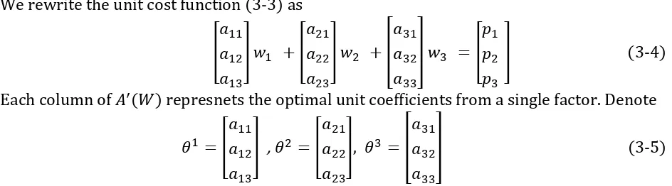
We rewrite the unit cost function (3-3) as
[ 𝑎11
𝑎12
𝑎13
] 𝑤1 + [
𝑎21
𝑎22
𝑎23
] 𝑤2 + [
𝑎31
𝑎32
𝑎33
] 𝑤3 = [
𝑝1
𝑝2
𝑝3
] (3-4)
Each column of 𝐴′(𝑊) represnets the optimal unit coefficients from a single factor. Denote
𝜃1 = [𝑎𝑎11 12
𝑎13
] , 𝜃2 = [ 𝑎21
𝑎22
𝑎23
], 𝜃3 = [ 𝑎31
𝑎32
𝑎33
] (3-5)
[image:8.612.72.544.231.362.2]Those three vectors are the three rays or ridges that compose the price tetrahedron in Figure 2.
When a price lines on any ridge of the tetrahedron, such as
𝑝 = 𝜃1 (3-6)
There are no rewards for factor 2 and factor 3 as
𝑤2 = 0, 𝑤3 = 0 (3-7)
When a price lines on any face (or surface) of the tetrahedron, such as
𝑝 = 𝜃1+ 𝜃2 (3-8)
There is no reward for factor 3. We see now that commodity price cannot line in any face of the price tetrahedron. It must lie within the tetrahedron.
3.3IWE box for the 3 x 3 x 2 Model
6 Integrated equilibriums allow the mobility of factor across countries. Our equilibrium analyses do not depend this
8
Figure 3 draws an Integrated World Equilibrium (IWE) for the 3 x 3 x 2 model. The origin for home country is the lower left corner, for country foreign is the right upper corner. Tetrahedra OMNR is the 3-dimension cone of factor endowments of country home and
Tetrahedra MNRO’ is for country foreign. Point E is the allocation of factor endowments of
the two countries. Point C is the supposed equilibrium point of trade.
3.4 Trade Box Specified by the Cone of Commodity Price through Shares of GNP
The first step for solving equilibrium in this study is to find the boundaries of shares of GNP, which identify a trade box, or a solution set of all trade equilibriums. We use the cone of commodity price doing this.
The definition of the share of GNP of a country is 𝑠ℎ = 𝑤′ 𝑉ℎ
𝑤′ 𝑉𝑊 (ℎ = 𝐻, 𝐹) (3-9)
Or
𝑠ℎ = 𝑃′ 𝑋ℎ
𝑃′ 𝑋𝑊 (ℎ = 𝐻, 𝐹) (3-10)
Giving a commodity price alone a ridge in the cone of commodity price, there is a boundary of the share of GNP. To calculate the boundaries of the share of GNP of country home, just let 𝑃 = 𝜃1, and substituting it into (3-10), we obtain the first boundary of the share of GNP as
𝑠1𝐻(𝜃1 ) = 𝜃
1′ 𝑋ℎ
𝜃1′ 𝑋𝑊 =
𝑣1𝐻
𝑣1𝑤 (3-11)
Similarly, for 𝑃 = 𝜃2 , we have
𝑠2𝐻(𝜃2) =𝑣2𝐻
𝑣2𝑤 (3-12)
9 𝑠3𝐻(𝜃3) =𝑣3
𝐻
𝑣3𝑤 (3-13)
We present the limits of the share of GNP in Figure 4. Using the scales of the three share of GNP, we draw a trade box indicated by NEMJRQ. All possible trade equilibrium points, like C, should fill (end) in the diagonal line QM.
[image:10.612.178.457.167.418.2]3.4GNP redistribution triangle for three commodities and three factors
Figure 5 displays the GNP distributions of the two countries by the trade box by
2-dimenssion. The vertical axis is the share of GNP of country foreign, and the horizontal axis is the share of GNP of country home.
The triangle ABC shows all possible GNPs of two countries, corresponding to all possible commodity price. We call it the GNP redistribution triangle. At any allocation of shares of GNP in the triangle ABC, there is always
𝑠𝐻+ 𝑠𝐹 = 1 (3-14)
The point 𝑠 is the centroid of triangle i.e. intersection of medians. Its allocation in the
triangle is
𝑠 = (𝑠𝐻, 𝑠𝐹) (3-15)
where
𝑠𝐻 =1 3(
𝑣1𝐻
𝑣1𝑤+
𝑣2𝐻
𝑣2𝑤+
𝑣3𝐻
𝑣3𝑤) (3-16) 𝑠𝐹 =1
3( 𝑣1𝐹
𝑣1𝑤+𝑣2 𝐹
𝑣2𝑤+𝑣3 𝐹
𝑣3𝑤) (3-17)
10
[image:11.612.174.428.78.322.2]Trades do redistribute welfare. The national welfare is measured by shares of GNP.
Figure 6 is the projection of the 3-dimension IWE in Figure 3, on the plane by
𝑣
1𝑤and
𝑣
2𝑤11
The trade box 𝐸𝐶𝑏𝑄𝐶𝑎 is the projection of trade box in Figure
4.
𝛼1is redistributable partof the share of GNP for the home country, and 𝛽1is for the foreign country.
When any 𝛼1 increases, the distributable share of GNP of country home will increase. In
addition, when any 𝛽1 increases, the distributable share of GNP of country foreign will
increase. The analyses will be similar, when we project the 3-dimenssion IWE on 𝑣2𝑤𝑣3𝑤
-plane and 𝑣1𝑤𝑣3𝑤-plane. Figure 6 only reflects competitive relation of a pair of factors
content of trade.
The lengths of redistributable GNP of for the home countries in three planes (
𝑣
1𝑤𝑣
2𝑤-plane,
𝑣
2𝑤𝑣
3𝑤-plane, and
𝑣
1𝑤𝑣
3𝑤-plane)
are 𝛼1 = (𝑠 −𝑣1𝐻
𝑣1𝑤), 𝛼2 = (𝑠 −𝑣2 𝐻
𝑣2𝑤), 𝛼3 = (𝑠 −𝑣3 𝐻
𝑣3𝑤) (3-18)
The lengths of redistributable GNP of for the home countries are 𝛽1 = (𝑣1
𝐻
𝑣1𝑤− 𝑠), 𝛽2 = (𝑣2 𝐻
𝑣2𝑤− 𝑠), 𝛽3 = (𝑣3 𝐻
𝑣3𝑤− 𝑠) (3-19)
We propose a utility function as
µ = 𝛼1𝛽1+ 𝛼2𝛽2+ 𝛼3𝛽3 (3-20)
It reflects the competitive relations of three pairs of factor content of trade, together. Trades do redistribute countries welfare. A country participating in trade tends better welfare. The share of GNP measures national welfare comprehensively.
Substituting (3-18) and (3-19) into (3-20) yields µ = (𝑣1𝐻
𝑣1𝑤− 𝑠) (𝑠 −
𝑣2𝐻
𝑣2𝑤) + (
𝑣3𝐻
𝑣3𝑤− 𝑠) (𝑠 −
𝑣2𝐻
𝑣2𝑤) + (
𝑣1𝐻
𝑣1𝑤− 𝑠) (𝑠 −
𝑣3𝐻
𝑣3𝑤) (3-21)
The optimal solution is by
𝑑µ
𝑑𝑠 = −2𝑠ℎ+ (
𝑣1𝐻
𝑣1𝑊+
𝑣2𝐻
𝑣2𝑊) − 2𝑠
ℎ+ (𝑣1𝐻
𝑣1𝑊+
𝑣2𝐻
𝑣2𝑊) − 2𝑠
ℎ+ (𝑣1𝐻
𝑣1𝑊+
𝑣2𝐻
𝑣2𝑊) = 0 (3-22)
There is
𝑠ℎ =1 3(
𝑣1𝐻
𝑣1𝑤+
𝑣2𝐻
𝑣2𝑤+
𝑣3𝐻
𝑣3𝑤) (3-23)
Therefore, the optimal competitive share of GNP of country home allocated at point
𝑠(𝑠𝐻, 𝑠𝐹) in Figure 5, which is the intersection of medians or centroid of the triangle. With
this simple competitive solution, both countries reach their maximum values of GNP shares in the box.
The maximization of the utility function (3-20) under conditions (3-18) and (3-19)
actually is a simple linear-quadratic one-step differential game, 𝑠ℎ is the equilibrium strategy,
which is optimal simultaneously for two players.
For the 2x2x2 model, the share of GNP, at the equilibrium, fits in the middle of the two boundaries of shares of GNP. There are two explanations of why it filled in the middle. One is that at this point, the redistributed shares of GNP of the two countries get their
12
3.5Generalizing the economics Logic in the 2 x 2 x 2 model
Factor content of trade is
𝐹𝐻= 𝑉𝐻− 𝑠𝐻𝑉𝑊 (3-24)
The trade balance condition by factor contents can be expressed as
(𝑣1𝐻− 𝑠𝐻𝑣1𝑤)𝑤1 + (𝑣2𝐻− 𝑠𝐻𝑣2𝑤)𝑤2 + (𝑣3𝐻− 𝑠𝐻𝑣3𝑤)𝑤3 = 0 (3-25)
For two-factor model, we can use trade balance to get a relative factor price as the term of factor content of trade. By equation (3-25), we cannot attain this, since there are three unknown-variables within it. We cannot obtain factor prices even when we know the trade volumes by the share of GNP (3-23). This is a challenge.
The whole 3 x 3 x 2 model is composed by production constraint (3-1), unit cost (3-2), and
trade balance7 (3-25). There are 13 endogenous (unknown) variables, 𝑝
𝑖 ∗, 𝑤
𝑖∗ , 𝑥𝑖ℎ,s, where
ℎ = 𝐻, 𝐹 and i=1,2. The model provides 10 constraint conditions. With the Walras’ law, we
can drop a market clearing condition by using a numericia. We suppose that 𝑤3∗ = 1. In
addition, we had figure out the share of GNP by (3-23). Totally, we get 12 conditions. We still need another condition (or equation) to determine the solution mathematically. (When factor number goes higher, we will miss more conditions.)
For the 2 x 2 x 2 model, we knew 𝑟∗/𝑤∗ = 𝐿𝑤/𝐾𝑤. It displays that a relative price of two
factors equals inversely to their amounts of factor endowments. We now generalize it to that a relative price of a pair of factors equals inversely to the amounts of their factor endowments, in the following relationship,
𝑤1∗ = 𝑤𝑤1∗
3∗ =
𝑣3𝑤
𝑣1𝑤 (3-26)
𝑤2∗= 𝑤2∗
𝑤3∗ =
𝑣3𝑤
𝑣2𝑤 (3-27)
𝑤3∗ = 𝑤𝑤3∗
3∗= 1 (3-28)
We need to prove it mathematically.
Firstly, we can demonstrate that factor price (3-26) through (3-27) satisfy the trade balance,
𝐹ℎ′𝑊∗ = 0 (ℎ = 𝐻, 𝐹) (3-29)
𝑇ℎ′𝑃∗ = 0 (ℎ = 𝐻, 𝐹) (3-30)
where trade volumes 𝑇ℎ and factor contents of trade 𝐹ℎ are calculated by using the share
of GNP by (3-23). Appendix A provide the details of the proofs for (3-29) and (3-30).
Secondly, we illustrate that the share of GNP calculated by (3-23) equals the share of GNP calculated by (3-9), so
𝑠𝐻=1 3(
𝑣1𝐻
𝑣1𝑤+𝑣2 𝐻
𝑣2𝑤+𝑣3 𝐻
𝑣3𝑤) = 𝑊∗′ 𝑉𝐻/𝑊∗′ 𝑉𝑊 (3-31)
The share of GNP (3-23) and the share of GNP by factor price (3-9) point to one result. They are from different logic. Therefore, this result is another cross-check. Appendix B provides the proof for (3-31).
7 The share of GNP (3-10) is not an independent condition from the trade balance condition
13
Thirdly, the factor prices in (3-26) and (3-28) is the Dixit-Norman price. They are
determined by world factor endowments. All allocations of factor endowments in IWE box in Figure 3 shares one world price. This is more important. It implies that the equalized factor price at the equilibrium is ascertained by the Dixit-Norman price. If a solution were not with this property, it was not the right equilibrium solution for the Heckscher-Ohlin model.
The solution satisfies all requirements of equilibrium from all aspects.
Actually, we can weak the assumptions 26) through 28). We drop the assumption (3-26). We only assume (3-27) and (3-28).
From (3-25), 𝑤1∗ can be calculated by
𝑤1∗ = −(𝑣2
𝐻− 𝑠𝐻𝑣
2𝑤)𝑤2+(𝑣3𝐻− 𝑠𝐻𝑣3𝑤)𝑤3
𝑣1𝐻− 𝑠𝐻𝑣1𝑤 (3-32)
Numerically for a giving example, we can demonstrate 𝑤1∗ =𝑣3𝑤
𝑣1𝑤 (3-33)
3.6 Equilibrium Solution
Substituting factor prices (3-26) through (3-28) into (3-3), we obtain commodity price
[𝑝1
∗
𝑝2∗
𝑝3∗
] = [ 𝑎11 𝑎21 𝑎31 𝑎12 𝑎22 𝑎32 𝑎13 𝑎23 𝑎33 ] ′ [
𝑣3𝑤
𝑣1𝑤
𝑣3𝑤
𝑣2𝑤 1 ]
(3-34)
Both factor price and commodity price at the equilibrium are the functions of world factor endowments, so the world prices are the Dixit-Norman IWE price.
With 𝑠ℎin (3-23), the trade volume and the net factor content of trade can be determined
by (3-24).
3.7Trade Pattern
From equation (3-18), the factor content of trade for commodity 1 is
𝐹1𝐻= 𝑣1𝐻− 𝑠ℎ𝑣1𝑤= 𝑣1𝐻−13(𝑣1 𝐻
𝑣1𝑤+𝑣2
𝐻
𝑣2𝑤+𝑣3
𝐻
𝑣3𝑤) 𝑣1𝑤 (3-35)
To study its trade pattern by assuming 𝐹1𝐻> 0, we obtain the following from above as
𝑣1𝐻
𝑣1𝑤>
1 3(
𝑣1𝐻
𝑣1𝑤+
𝑣2𝐻
𝑣2𝑤+
𝑣3𝐻
𝑣3𝑤) (3-36)
It can be simplified as
𝑣1𝐻
𝑣1𝑤 >
3 2(
𝑣2𝐻
𝑣2𝑤+
𝑣3𝐻
𝑣3𝑤) (3-37)
Therefore, if inequality (3-36) is true, country 1’net factor content of trade is positive. It is a
14
For commodity trade direction, we use commodity 1 as an example,
𝑥1ℎ− 𝑠𝑥1𝑤= 𝑥1ℎ−13(𝑣1 𝐻
𝑣1𝑤+𝑣2 𝐻
𝑣2𝑤+𝑣3 𝐻
𝑣3𝑤) 𝑥1𝑤 (3-38)
To study its trade pattern by assuming 𝑥1𝐻−𝑠𝑥1𝑤> 0, we rewrite (3-32) as
𝑥1ℎ 𝑥1𝑤>
1 3(
𝑣1𝐻
𝑣1𝑤+
𝑣2𝐻
𝑣2𝑤+
𝑣3𝐻
𝑣3𝑤) (3-39)
The easy description of the trade direction is that if a country’s relative share of a
commodity output to the world output is greater than its share of GNP, it exports that commodity.
3.8A numerical example
Let see a numerical example for the 3x3x2 model. The identical technology matrix in this example is
𝐴 = [2.7 1.2 1.11.3 2.0 1.0 1.1 1.5 1.8] The factor endowments for the two countries are
𝑉𝐻 = [38003900
4300]
, 𝑉𝐹 = [34004300 4000]
The commodity outputs of two countries by the factor resources under full employment are
[𝑥1
𝐻
𝑥2𝐻
𝑥3𝐻
] = [1025.95422.01
1299.48], [ 𝑥1𝐹
𝑥2𝐹
𝑥3𝐹
] = [1630.15236.34 732.47] Calculating the factor price directly from (3-20) through (3-22) yields
[𝑤1
∗
𝑤2∗
𝑤3∗
] = [1.15271.0121 1.0000]
Based on the equalized factor price above, we can obtain the world common commodity price by (3-27) as
[𝑝1
∗
𝑝2∗
𝑝3∗
] = [5.42834.9077 4.0802]
With the prices above, we can calculate the share of GNP of country home from (3-9) as s1 = 0.5071
By the shares of GNP, the exports and factor contents of exports will be
[ 𝑇1𝐻
𝑇2𝐻
𝑇3𝐻
] = − [ 𝑇1𝐻
𝑇2𝐻
𝑇3𝐻
] = [−321.1088.13 268.97 ]
[𝐹1
𝐻
𝐹2𝐻
𝐹3𝐻
] = − [𝐹1
𝐻
𝐹2𝐻
𝐹3𝐻
] = [−258.65148.49
15
4. World Trade Space and Integrated World Trade Equilibrium
Let discuss the general equilibrium of trade for the scenario of m factors, n commodities, and q countries (the N x M x Q) model) now.
The technology matrix for n commodity and m factor can be expressed as
𝐴 =
[
𝑎11 𝑎12 ⋯ 𝑎1𝑚
𝑎21 𝑎22 ⋯ 𝑎2𝑚
⋱ 𝑎𝑛1 𝑎𝑛2 ⋯ 𝑎𝑛𝑚]
(4-1)
The commodity vector and the commodity price vector are the m x 1 vectors as
𝑃𝑤 = [ 𝑝1ℎ
𝑝2ℎ
⋮ 𝑝𝑚ℎ]
, 𝑋ℎ =
[ 𝑥1ℎ
𝑥2ℎ
⋮ 𝑥𝑚ℎ]
ℎ = (1,2, ⋯ , q)
where h indicates countries.
Factor endowments and factor prices are the n x 1 vectors as
𝑉ℎ = [ 𝑣1ℎ
𝑣2ℎ
⋮ 𝑝𝑛ℎ]
, 𝑊ℎ =
[ 𝑤1ℎ
𝑤2ℎ
⋮ 𝑤𝑛ℎ]
ℎ = (1,2, ⋯ , q)
Production constraint is
𝐴𝑋ℎ = 𝑉ℎ (4-2) Unit cost function at factor price equalization is
𝐴′ 𝑊∗ = 𝑃∗ (4-3) To establish the trade equilibrium, we start at identifying n boundaries of shares of GNP of country h. Denote
𝜃1 =
[ 𝑎11
𝑎12
⋮ 𝑎1𝑚]
, 𝜃2 =
[ 𝑎21
𝑎22
⋮ 𝑎2𝑚]
, …. 𝜃𝑛 =
[ 𝑎𝑛1
𝑎𝑛2
⋮ 𝑎𝑛𝑚]
(4-4)
Substituting them into the definition of the share of GNP like (3-10) for country h yields
𝑠1ℎ(𝜃1) = 𝑣1
ℎ
𝑣1𝑤 , 𝑠2ℎ(𝜃2) = 𝑣2ℎ
𝑣2𝑤 , …. , 𝑠𝑛ℎ(𝜃𝑛) = 𝑣𝑛ℎ
𝑣𝑛𝑤 , ℎ = (1,2, ⋯ , 𝑞) (4-5)
Generalizing the result of utility function (3-21), we can obtain the share of GNP in the following,
𝑠ℎ = 1 𝑛∑
𝑣𝑖𝐻 𝑣𝑖𝑤 𝑛
𝑖=1 (4-6)
Suppose the factor n’s reward is unity as
𝑤𝑛∗ = 1 (4-7)
16 𝑤𝑗∗ = 𝑣𝑣𝑛𝑤
𝑗𝑤 𝑗 = (1,2, ⋯ , 𝑛 − 1) (4-8)
We can prove that trade balance for country h can be satisfied by the above factor prices8
as
𝐹ℎ′𝑊∗ = 0 ℎ = (1,2, ⋯ , 𝑞) (4-9)
The common commodity price can be expressed as
𝑃∗ = 𝐴′𝑊∗ = [
𝑝1∗
𝑝2∗
⋮ 𝑝𝑚∗
] = [
𝑎11 𝑎21 ⋯ 𝑎𝑚1
𝑎11 𝑎22 ⋯ 𝑎𝑚2
⋮ ⋮ ⋱ ⋮
𝑎1𝑚 𝑎2𝑚 ⋯ 𝑎𝑚𝑛]
[
𝑣𝑛𝑤⁄𝑣1𝑤
𝑣𝑛𝑤⁄𝑣2𝑤
⋮ 1
] (4-10)
Equations (4-7), (4-8), and (4-10) are the world commodity price and factor price of world trade equilibrium. Price (4-10) satisfy the commodity trade balance as
𝑇ℎ′𝑃∗ = 0 ℎ = (1,2, ⋯ , 𝑞) (4-11)
World price (equalized factor price and common commodity price) are the same for all countries. In the above analyses, we only specify country h in general. The shares of GNP (4-6) are different from country to country. The world prices are functions of world factor endowments. It is globally unique, all countries.
The trade volume for commodity j for country ℎ is
𝑇𝑗ℎ = 𝑥𝑗ℎ− 𝑠ℎ𝑥𝑗𝑤= 𝑥𝑗ℎ−1𝑛𝑥𝑗𝑤∑ 𝑣𝑖 ℎ
𝑣𝑖𝑤
𝑛
𝑖=1 (4-13)
The factor content of trade for factor j in for country ℎ is
𝐹𝑗ℎ = 𝑣𝑗ℎ− 𝑠ℎ𝑣𝑗𝑤= 𝑣𝑗ℎ−1𝑛𝑣𝑗𝑤∑ 𝑣𝑖 ℎ
𝑣𝑖𝑤 𝑛
𝑖=1 (4-14)
The shares of GNP by (4-6) for all countries are harmony, summing them together equals to 1 as
∑ (1𝑛∑ 𝑣𝑖ℎ
𝑣𝑖𝑤
𝑛
𝑖=1 ) = 1
𝑞
ℎ=1 (4-15)
The commodity price (4-10) do not need the assumption that technological matrix A is squared.
5. Autarky Price and Gains From Trade
Guo (2018) proposed a way to estimate autarky price by the logic that world factor resource determine world price. His argument is that the autarky resource of factor endowments determines autarky price.
Samuelson (1949) made arguments about factor price equalization and outlines his
description of autarky trade equilibrium. He reasoned that an angel’s recording geographer
device notified some fraction of all factor endowments, one is called American, the rest to
be Europeans. “Obviously, just giving people and areas national label does not alter
anything; it does not change commodity or factor prices or production patterns, but with
identical real wage and rents and identical modes of commodity production. ... [W]hat will
be the result? Two countries with quite different factor proportions, but with identical real
17
wages and rents and identical modes of commodity production (but with different relative importance of food and clothing industries). ... Both countries must have factor proportions intermediate between the proportions in the two industries. The angel can create a country with proportions not intermediate between the factor intensities of food and clothing. But he cannot do so by following the above-described procedure, which was calculated to leave
prices and production unchanged." He mentioned, “to leave prices and production
unchanged” with emphasis. He implies that autarky price of the kingdom is the world price of countries by artificial map or labels of the recording geographer device.
The IWE itself supports the logic that autarky factor resource determines autarky price
analytically. Suppose that one country shrinks to very small. Another country’s autarky
price is then the world price of the current trade. Mathematically, when 𝑉𝐻→ 0, inside the
IWE box, then 𝑉𝐹 → 𝑉𝑊 and 𝑃𝐹𝑎 → 𝑃∗. So far, we (almost) proof the autarky price
mathematically.
Let us examine gains from trade for the 3 x 3 x 2 model. By the logic that autarky factor endowments determine autarky price, the autarky prices will be
[𝑤1
ℎ𝑎
𝑤2ℎ𝑎
𝑤3ℎ𝑎
] = [
𝑣3ℎ
𝑣1ℎ 𝑣3ℎ
𝑣2ℎ
1 ]
ℎ = (𝐻, 𝐹) (5-1)
[𝑝1
ℎ𝑎
𝑝2ℎ𝑎
𝑝3ℎ𝑎
] = [ 𝑎11
𝑎21
𝑎31
𝑎12
𝑎22
𝑎32
𝑎13
𝑎23
𝑎33
]
′
[
𝑣3ℎ
𝑣1ℎ
𝑣3ℎ 𝑣2ℎ
1 ]
ℎ = (𝐻, 𝐹) (5-2)
From the relations, 𝑉𝐻+ 𝑉𝐹 = 𝑉𝑊, we can easily to see that the home factor endowment
𝑉𝐻, the foreign factor endowment 𝑉𝐹, and world factor endowment 𝑉𝑊are coplanar, i.e.
they are in a same surface. Similarly, we see that the home commodity vector 𝑋𝐻, the
foreign commodity vector, 𝑋𝐹, and the world commodity vectors, 𝑋𝑊 ,are coplanar.
In addition, the numerical studies of this paper show that the autarky commodity prices of
two countries, 𝑃𝐻𝑎and 𝑃𝐹𝑎, and world commodity price, 𝑃∗ are coplanar9; autarky factor
prices of two countries 𝑊𝐻𝑎and 𝑊𝐹𝑎 and the equalized factor price, 𝑊∗, are coplanar.
This means that the world factor price lies between the rays of the cone of autarky factors prices of two countries.
9This needs an “absolution” price references. Autarky price should be based on
𝑤1ℎ𝑎 = 𝑣1
1
ℎ𝑎 , 𝑤2ℎ𝑎 =𝑣1
2ℎ𝑎 , 𝑤3
ℎ𝑎 = 1 𝑣3ℎ𝑎
World common price should be based on 𝑤1∗ =𝑣1
1∗ , 𝑤2
∗ = 1
𝑣2∗ , 𝑤3
18
The autarky commodity prices of two countries and world commodity price all should fill the cone (the tetrahedron) of commodity price in Figure 2. The coplanar by
𝑃𝐻𝑎, 𝑃𝐹𝑎, 𝑎𝑛𝑑 𝑃∗ will cut through the cone (the tetrahedron) of commodity price. This is
helpful to understand gains from trade.
Calculating the shares of GNP by the autarky prices of two countries yields, 𝑠𝐻𝑎= 𝑠𝐻𝑎(𝑝𝐻𝑎)
𝑠𝐹𝑎 = 𝑠𝐹𝑎(𝑝𝐹𝑎)
where 𝑠ℎ𝑎 is the share of GNP by autarky price for country h.
We draw them on the trade box in Figure 7. If the trade vector lies on line AB, both countries will receive gains from trade. The price solution (3-28) naturally lies in the line AB.
Let see a numerical example of gains from trade. We still use the case in the last section. The autarky factor price and commodity price of two countries, by the logic that autarky factor endowments determine autarky price, will be
[𝑤1
𝐻𝑎
𝑤2𝐻𝑎
𝑤3𝐻𝑎
] = [1.13131.1021
1.0000], [ 𝑤1𝐹𝑎
𝑤2𝐹𝑎
𝑤3𝐹𝑎
] = [1.17640.9302 1.0000]
[ 𝑝1𝐻𝑎
𝑤2𝐻𝑎
𝑤3𝐻𝑎
] = [5.42835.0630
4.1473], [ 𝑝1𝐹𝑎
𝑝2𝐹𝑎
𝑤3𝐹𝑎
] = [5.38574.7772 4.0243] The gains from trade for the two countries will be
−𝑊ℎ𝑎′𝐹ℎ= −[1.1313 1.1021 1.0000] [−258.65148.49
19
−𝑃ℎ𝑎′𝑇ℎ= −[5.4283 5.0630 4.1473] [−321.1088.13
268.97 ] = 26.52 > 0
−𝑊𝐹𝑎′𝐹𝐹= [1.1764 0.9302 1.0000] [−258.65148.49
90.62 ] = 24.71 > 0
−𝑃𝐹𝑎′𝑇𝐹= [5.3857 4.7772 4.0243] [−321.1088.13
268.97 ] = 24.71 > 0
We add the negative sign in inequalities above since we expressed trade by net export, 𝑇ℎ .
In most other literatures, they express trade by net import.
Appendix D is another numerical example to display gains from trade. It is a model with 4 factors, 5 commodities, and 3 countries.
6. Discussions
The general equilibrium and the world factor price equalization are attained for the 𝑁 ×
𝑀 × 𝑄 Heckscher-Ohlin space. It means that the equalized factor price is anywhere for Heckscher-Ohlin models, and the gains from trade are anywhere for any Heckscher-Ohlin trade. The solution is much simple than expected. The price structure of the PFE sourced from the Heckscher-Ohlin model structure.
Dixit (2010) and Jones (1983) thought that the factor-price equalization theorem should produce the result of Heckscher-Ohlin theorem and that the idea was implicit there. The equalized factor price at the equilibrium does present the trade pattern with trade volume. The trade equilibrium of this paper proofs the Heckscher-Ohlin theorem and the Factor Price Equalization theorem together. Behind the world commodity trade, the world factor-endowment resources, fully employed, determine world price.
It is said that the Heckscher-Ohlin theory is a positive trade theory to identify it from the Ricardo trade theory. Heckscher and Ohlin original studies made their efforts and
contributions on the comparative advantage for their model. Their price definition of capital abundant is the most related idea about the comparative advantage. Much
literature proofed the conditions of gains from trade for the Heckscher-Ohlin model; this paper illustrated it quantitatively by specifying the reasonable autarky price.
The equalized factor price and world commodity price at the equilibrium ensure gains from trade. The countries with comparative advances in production sourced from factor
endowment difference, export respective commodities.
We propose a theorem to summarize the result of the general equilibrium of this study.
The IWE comparative advantage theorem
At the equilibrium, the FPE reached as the Dixit-Norman price. The world factor
20
commodity price) that assure the gains from trade for countries participated in trade. Each country participating in free trade exports commodities with comparative advantage to produce them by factor endowments different across countries.
Proof
The solution is unique for a giving IWE box. The world prices as the functions of world factor endowments are globally identical for each country. The numerical examples of the 3 x 3 x 2 model in section 5 and the 4 x 5 x 3 model in Appendix 4 provide the calculation result of gains from trade. Guo(2018) had proofed the gains from trade for the 2 x 2 x 2 model analytically.
End
The IWE comparative advantage theorem is a joint statement of the Heckscher-Ohlin theorem and the factor-price equalization theorem. The equalized factor price at the equilibrium is the Dixit-Norman price.
Conclusion
The Heckscher-Ohlin trade theory, in particular, has frequently been criticized for the restriction to the lower dimension presentations. This study provides the understanding of trade-price relationships for higher dimensions model.
This paper draws a simple picture of world trade flows for complexed world trade
practices. It shows that the Heckscher-Ohlin model and theories have the capacity to reflect real international trade in the framework of higher dimensions, from trade volumes, world prices, to gains from trades.
Woodland (2011) mentioned that from a theory perspective, the factor price equalization is a prediction of the model rather than an assumption. This study proofs the prediction in the higher dimensions. The solution is affirmed by the Dixit-Norman price inference theoretically. This is more important than the methodology used in this study.
The study consolidated the Heckscher-Ohlin theorems. It states trade directions with trade volumes; it presented the equalized factor prices with its price structure; it established that the equalized factor price at the equilibrium makes sure of gains from trade for all
countries participating in trade.
Appendix A - The derivations for the trade balance
A1 Trade Balance by Factor Price
Trade balance is
21
The factor 1 content of trade in country h by the share of GNP in (3-23) is
𝐹1𝐻= 𝑣1𝐻− 𝑠ℎ𝑣1𝑤= 𝑣1𝐻−13(𝑣1 𝐻
𝑣1𝑤+𝑣2
𝐻
𝑣2𝑤+𝑣3
𝐻
𝑣3𝑤) 𝑣1𝑤 (A-2)
Timing two sides of the above by two sides of equation (3-26), we obtain,
𝐹1𝐻𝑤1∗=𝑣1
𝐻
𝑣1𝑤𝑣3𝑤−13(𝑣1
𝐻
𝑣1𝑤+𝑣2 𝐻
𝑣2𝑤+𝑣3 𝐻
𝑣3𝑤)𝑣3𝑤 (A-3)
Similarly, we can obtain
𝐹2𝐻𝑤2∗=𝑣2
𝐻
𝑣2𝑤𝑣3𝑤−13(𝑣1
𝐻
𝑣1𝑤+𝑣2 𝐻
𝑣2𝑤+𝑣3 𝐻
𝑣3𝑤)𝑣3𝑤 (A-4)
𝐹3𝐻𝑤3∗=𝑣3
𝐻
𝑣3𝑤𝑣3𝑤−13(𝑣1
𝐻
𝑣1𝑤+𝑣2
𝐻
𝑣2𝑤+𝑣3
𝐻
𝑣3𝑤)𝑣3𝑤 (A-5)
Summing (A-2), (A-3) and (A4), we obtain
𝐹′𝑊 = ∑ 𝐹
𝑖 ℎ𝑤𝑖∗
3
𝑖=1 = 0 (A-6)
A2 Trade Balance by Commodity Price
The trade balance by commodity price is
𝑇ℎ′𝑃 = 0 (A-7)
Transposing (A-7) yields
𝐹ℎ′ = 𝑇ℎ′𝐴′ (A-8)
Right time W two sides of (A-8) yields
𝐹ℎ′𝑊 = 𝑇ℎ′𝐴′𝑊 (A-9)
The left side (A-8) is
𝐹ℎ′𝑊 = 0 (A-10)
Therefore, right side (A-8) is
𝑇ℎ′𝐴′𝑊 = 𝑇ℎ′𝑃 = 0 (A-11)
Appendix B – Share of GNP by the factor price
The definition of share of GNP for country h is
𝑠ℎ = 𝑊′ 𝑉ℎ/𝑊′ 𝑉𝑊 (A-12)
The numerator in (A-12) is
𝑊′𝑉ℎ= (𝑣1𝐻)𝑣3 𝑤
𝑣1𝑤+(𝑣2𝐻)𝑣3 𝑤
𝑣2𝑤+(𝑣3𝐻)𝑣3 𝑤
𝑣3𝑤=(𝑣1 𝐻
𝑣1𝑤+𝑣2 𝐻
𝑣2𝑤+𝑣3 𝐻
𝑣3𝑤)𝑣3𝑤 (A-13)
The denominator in (A-12) is
𝑊′𝑉𝑤= (𝑣1𝑤)𝑣3 𝑤
𝑣1𝑤+(𝑣2𝑤)𝑣3 𝑤
𝑣2𝑤+(𝑣3𝑤)𝑣3 𝑤
𝑣3𝑤= 3𝑣3𝑤 (A-14)
Substituting (A-13) and (A-14) into (A-12) yields 𝑠𝐻 = 13(𝑣1𝐻
𝑣1𝑤+
𝑣2𝐻
𝑣2𝑤+
𝑣3𝐻
𝑣3𝑤) (A-15)
22 Appendix C - Gains from trade for the 4 x 5 x 3 model
Let see a numerical example for the 4 x 5 x 3 model. The identical technology matrix in this example is
𝐴 = [
3.0 1.2
1.1 2
0.8 1.1
1.3 0.9 0.7 1.1 1.1 1.0 2.1 1.0 1.2 1.3 1.0 0.8 1.5 1.1 ]
The commodity outputs of three countries by full employment of factor resources are given in advance as
𝑋1 =
[ 600 1300 410 400 560 ]
, 𝑋2 =
[ 250 540 1490 600 800 ]
, 𝑋3 =
[ 900 600 500 1000 1500] The factor endowments for the three countries correspondingly are
V1 = [
4655 4711 3843 3624
], V2 = [ 4435 4454 5483 3837
] , V3 = [ 6020 5340 5230 5320
]
Calculating the factor price directly from (3-20) through (3-22) yields
𝑊∗ = [
0.8464 0.8811 0.8780
1 ]
Based on the equalized factor price above, we can obtain the world common commodity price as
𝑃∗ =
[ 5.5109 4.7438 4.7135 4.1090 3.6273]
With the prices above, we can calculate the share of GNP of each country as 𝑠1 = 0.2949
𝑠2 = 0.3194
𝑠3 = 0.3855
We can also use (4-6) to calculate the shares of GNP; the results are same as above. The exports and factor contents of exports will be
𝑇1 =
[ 83.77 583.22 −297.98 −189.98 −238.67]
, 𝑇2 =
[ −308.98 −239.38 723.40 −38.83 −113.53]
, 𝑇3 =
[ 225.21 −340.85 −425.42 228.82 397.21 ]
𝐹1 = [
190.64 432.16 −450.87 −146.27
], 𝐹2 = [
−388.20 −179.14 833.56 −245.47
]. 𝐹3 = [
197.55 −253.01 −382.68 391.74
]
23 𝑃1𝑎 =
[
5.5109 4.7438 4.7135 4.1090 3.6273]
, 𝑃2𝑎 =
[
5.5109 4.7438 4.7135 4.1090 3.6273]
, 𝑃3𝑎 =
[
5.5109 4.7438 4.7135 4.1090 3.6273]
𝑊1𝑎 = [
0.8464 0.8811 0.8780
1
], 𝑊2𝑎 = [
0.8464 0.8811 0.8780
1
], 𝑊3𝑎 = [
0.8464 0.8811 0.8780
1 ]
The gains from trade for the three countries will be
−𝑊1𝑎′𝐹1= −𝑃1𝑎′𝑇1= 90.26 > 0
−𝑊2𝑎′𝐹2= −𝑃2𝑎′𝑇2= 152.33 > 0
−𝑊3𝑎′𝐹3= −𝑃3𝑎′𝑇3= 75.00 > 0
Reference
McKenzie, L. (1987), General Equilibrium, The New Palqrave, A dictionary of economics, 1987, v. 2, pp 498-512.
Chipman, J. S. (1966), “A Survey of the Theory of International Trade: Part 3, The Modern
Theory”, Econometrica 34 (1966): 18-76.
Chipman, J. S. (1969), Factor price equalization and the Stolper–Samuelson theorem.
International Economic Review, 10(3), 399−406.
Deardorff, A. V. (1979), Weak Links in the chain of comparative advantage, Journal of international economics. IX, 197-209.
Deardorff, A. V. (1994), The possibility of factor price equalization revisited, Journal of International Economics, XXXVI, 167-75.
Etheir, W. (1984). Higher dimensional issues in the trade theory, Ch33 in handbook of international Economics, Vol. 1, ed. R. Jones and P. Kenen, Amsterdam: North-Holland.
Dixit, A.K. and V. Norman (1980) Theory of International Trade, J. Nisbert/Cambridge University Press.
Helpman, E. (1984), The Factor Content of Foreign Trade, Economic Journal, XCIV, 84-94.
Helpman, E. and P. Krugman (1985), Market Structure and Foreign Trade, Cambridge, MIT Press.
Guo, B. (2005), Endogenous Factor-Commodity Price Structure by Factor Endowments International Advances in Economic Research, November 2005, Volume 11, Issue 4, p 484
Guo, B. (2018), Equalized Factor Price and Integrated World Equilibrium, working paper,
24
Gale, D. and Nikaido, H. 1965. The jacobian matrix and the global univalence of mappings. Mathematishe Annalen 159, 81-93.
Jones, Ronald (1965), “The Structure of Simple General Equilibrium Models,” Journal of Political Economy 73 (1965): 557-572.
McKenzie, L.W. (1955), Equality of factor prices in world trade, Econometrica 23, 239-257.
Rassekh, F. and H. Thompson (1993) Factor Price Equalization: Theory and Evidence, Journal of Economic Integration: 1-32.
Samuelson, P.A. (1949), International factor price equalization once again, The Economic Journal 59, 181-197.
Schott, P. (2003) One Size fits all? Heckscher-Ohlin specification in global production, American Economic Review, XCIII, 686-708.
Takayama, A. (1982), “On Theorems of General Competitive Equilibrium of Production and
Trade: A Survey of Recent Developments in the Theory of International Trade,” Keio Economic Studies 19 (1982): 1-38. 10
Trefler, D. (1998), “The Structure of Factor Content Predictions,” University of Toronto,
manuscript.
Vanek, J. (1968b), The Factor Proportions Theory: the N-Factor Case, Kyklos, 21(23), 749-756.
Woodland, A. (2013), General Equilibrium Trade Theory, Chp. 3, Palgrave Handbook of International Trade, Edited by Bernhofen, D., Falvey, R., Greenaway, D. and U.