Active Learning with Efficient Feature Weighting Methods
for Improving Data Quality and Classification Accuracy
Justin Martineau1, Lu Chen2∗, Doreen Cheng3, and Amit Sheth4
1,3Samsung Research America, Silicon Valley 1,375 W Plumeria Dr. San Jose, CA 95134 USA
2,4Kno.e.sis Center, Wright State University 2,43640 Colonel Glenn Hwy. Fairborn, OH 45435 USA
1,3{justin.m, doreen.c}@samsung.com 2,4{chen, amit}@knoesis.org
Abstract
Many machine learning datasets are noisy with a substantial number of mislabeled instances. This noise yields sub-optimal classification performance. In this paper we study a large, low quality annotated dataset, created quickly and cheaply us-ing Amazon Mechanical Turk to crowd-source annotations. We describe compu-tationally cheap feature weighting tech-niques and a novel non-linear distribution spreading algorithm that can be used to it-eratively and interactively correcting mis-labeled instances to significantly improve annotation quality at low cost. Eight dif-ferent emotion extraction experiments on Twitter data demonstrate that our approach is just as effective as more computation-ally expensive techniques. Our techniques save a considerable amount of time. 1 Introduction
Supervised classification algorithms require anno-tated data to teach the machine, by example, how to perform a specific task. There are generally two ways to collect annotations of a dataset: through a few expert annotators, or through crowdsourc-ing services (e.g., Amazon’s Mechanical Turk). High-quality annotations can be produced by ex-pert annotators, but the process is usually slow and costly. The latter option is appealing since it creates a large annotated dataset at low cost. In recent years, there have been an increasing num-ber of studies (Su et al., 2007; Kittur et al., 2008; Sheng et al., 2008; Snow et al., 2008; Callison-Burch, 2009) using crowdsourcing for data anno-tation. However, because annotators that are re-cruited this way may lack expertise and motiva-tion, the annotations tend to be more noisy and
∗
This author’s research was done during an internship with Samsung Research America.
unreliable, which significantly reduces the perfor-mance of the classification model. This is a chal-lenge faced by many real world applications –
given a large, quickly and cheaply created, low quality annotated dataset, how can one improve its quality and learn an accurate classifier from it?
Re-annotating the whole dataset is too expen-sive. To reduce the annotation effort, it is desirable to have an algorithm that selects the most likely mislabeled examples first for re-labeling. The pro-cess of selecting and re-labeling data points can be conducted with multiple rounds to iteratively im-prove the data quality. This is similar to the strat-egy of active learning. The basic idea of active learning is to learn an accurate classifier using less training data. An active learner uses a small set of labeled data to iteratively select the most informa-tive instances from a large pool of unlabeled data for human annotators to label (Settles, 2010). In this work, we borrow the idea of active learning to interactively and iteratively correct labeling errors. The crucial step is to effectively and efficiently
select the most likely mislabeled instances. An in-tuitive idea is to design algorithms that classify the data points and rank them according to the decreasing confidence scores of their labels. The data points with the highest confidence scores but conflicting preliminary labels are most likely mis-labeled. The algorithm should be computationally cheap as well as accurate, so it fits well with ac-tive learning and other problems that require fre-quent iterations on large datasets. Specifically, we propose a novel non-linear distribution spread-ing algorithm, which first uses Delta IDF tech-nique (Martineau and Finin, 2009) to weight fea-tures, and then leverages the distribution of Delta IDF scores of a feature across different classes to efficiently recognize discriminative features for the classification task in the presence of misla-beled data. The idea is that some effective
tures may be subdued due to label noise, and the proposed techniques are capable of counteracting such effect, so that the performance of classifica-tion algorithms could be less affected by the noise. With the proposed algorithm, the active learner be-comes more accurate and resistant to label noise, thus the mislabeled data points can be more easily and accurately identified.
We consider emotion analysis as an interest-ing and challenginterest-ing problem domain of this study, and conduct comprehensive experiments on Twit-ter data. We employ Amazon’s Mechanical Turk (AMT) to label the emotions of Twitter data, and apply the proposed methods to the AMT dataset with the goals of improving the annotation quality at low cost, as well as learning accurate emotion classifiers. Extensive experiments show that, the proposed techniques are as effective as more com-putational expensive techniques (e.g, Support Vec-tor Machines) but require significantly less time for training/running, which makes it well-suited for active learning.
2 Related Work
Research on handling noisy dataset of mislabeled instances has focused on three major groups of techniques: (1) noise tolerance, (2) noise elimi-nation, and (3) noise correction.
Noise tolerance techniques aim to improve the learning algorithm itself to avoid over-fitting caused by mislabeled instances in the training phase, so that the constructed classifier becomes more noise-tolerant. Decision tree (Mingers, 1989; Vannoorenberghe and Denoeux, 2002) and boosting (Jiang, 2001; Kalaia and Servediob, 2005; Karmaker and Kwek, 2006) are two learn-ing algorithms that have been investigated in many studies. Mingers (1989) explores pruning methods for identifying and removing unreliable branches from a decision tree to reduce the influence of noise. Vannoorenberghe and Denoeux (2002) pro-pose a method based on belief decision trees to handle uncertain labels in the training set. Jiang (2001) studies some theoretical aspects of regres-sion and classification boosting algorithms in deal-ing with noisy data. Kalaia and Servediob (2005) present a boosting algorithm which can achieve arbitrarily high accuracy in the presence of data noise. Karmaker and Kwek (2006) propose a mod-ified AdaBoost algorithm – ORBoost, which min-imizes the impact of outliers and becomes more
tolerant to class label noise. One of the main dis-advantages of noise tolerance techniques is that they are learning algorithm-dependent. In con-trast, noise elimination/correction approaches are more generic and can be more easily applied to various problems.
A large number of studies have explored noise elimination techniques (Brodley and Friedl, 1999; Verbaeten and Van Assche, 2003; Zhu et al., 2003; Muhlenbach et al., 2004; Guan et al., 2011), which identifies and removes mislabeled examples from the dataset as a pre-processing step before build-ing classifiers. One widely used approach (Brod-ley and Friedl, 1999; Verbaeten and Van Assche, 2003) is to create an ensemble classifier that com-bines the outputs of multiple classifiers by either majority vote or consensus, and an instance is tagged as mislabeled and removed from the train-ing set if it is classified into a different class than its training label by the ensemble classifier. The similar approach is adopted by Guan et al. (2011) and they further demonstrate that its performance can be significantly improved by utilizing unla-beled data. To deal with the noise in large or distributed datasets, Zhu et al. (2003) propose a partition-based approach, which constructs clas-sification rules from each subset of the dataset, and then evaluates each instance using these rules. Two noise identification schemes, majority and non-objection, are used to combine the decision from each set of rules to decide whether an in-stance is mislabeled. Muhlenbach et al. (2004) propose a different approach, which represents the proximity between instances in a geometrical neighborhood graph, and an instance is consid-ered suspect if in its neighborhood the proportion of examples of the same class is not significantly greater than in the dataset itself.
Removing mislabeled instances has been demonstrated to be effective in increasing the classification accuracy in prior studies, but there are also some major drawbacks. For example, useful information can be removed with noise elimination, since annotation errors are likely to occur on ambiguous instances that are potentially valuable for learning algorithms. In addition, when the noise ratio is high, there may not be adequate amount of data remaining for building an accurate classifier. The proposed approach does not suffer these limitations.
from training data, some researchers (Zeng and Martinez, 2001; Rebbapragada et al., 2012; Lax-man et al., 2013) propose to correct labeling er-rors either with or without consulting human ex-perts. Zeng and Martinez (2001) present an ap-proach based on backpropagation neural networks to automatically correct the mislabeled data. Lax-man et al. (2012) propose an algorithm which first trains individual SVM classifiers on several small, class-balanced, random subsets of the dataset, and then reclassifies each training instance using a ma-jority vote of these individual classifiers. How-ever, the automatic correction may introduce new noise to the dataset by mistakenly changing a cor-rect label to a wrong one.
In many scenarios, it is worth the effort and cost to fix the labeling errors by human experts, in order to obtain a high quality dataset that can be reused by the community. Rebbapragada et al. (2012) propose a solution called Active Label Cor-rection (ALC) which iteratively presents the ex-perts with small sets of suspected mislabeled in-stances at each round. Our work employs a sim-ilar framework that uses active learning for data cleaning.
In Active Learning (Settles, 2010) a small set of labeled data is used to find documents that should be annotated from a large pool of unlabeled doc-uments. Many different strategies have been used to select the best points to annotate. These strate-gies can be generally divided into two groups: (1) selecting points in poorly sampled regions, and (2) selecting points that will have the greatest impact on models that were constructed using the dataset. Active learning for data cleaning differs from traditional active learning because the data already has low quality labels. It uses the difference be-tween the low quality label for each data point and a prediction of the label using supervised machine learning models built upon the low quality labels. Unlike the work in (Rebbapragada et al., 2012), this paper focuses on developing algorithms that can enhance the ability of active learner on identi-fying labeling errors, which we consider as a key challenge of this approach but ALC has not ad-dressed.
3 An Active Learning Framework for Label Correction
Let Dˆ = {(x1, y1), ...,(xn, yn)} be a dataset of binary labeled instances, where the instancexi
be-longs to domainX, and its labelyi ∈ {−1,+1}.
ˆ
D contains an unknown number of mislabeled data points. The problem is to obtain a high-quality datasetD by fixing labeling errors in Dˆ, and learn an accurate classifierCfrom it.
Algorithm 1 illustrates an active learning ap-proach to the problem. This algorithm takes the noisy dataset Dˆ as input. The training set T is initialized with the data in Dˆ and then updated each round with new labels generated during re-annotation. Data setsSrandS are used to main-tain the instances that have been selected for re-annotation in the whole process and in the current iteration, respectively.
Data: noisy dataDˆ
Result: cleaned dataD, classifierC
Initialize training setT = ˆD;
Initialize re-annotated data setsSr =∅;
S =∅;
repeat
Train classifierCusingT ;
UseCto select a setSofmsuspected mislabeled instances fromT ;
Experts re-annotate the instances in
S−(Sr∩S);
UpdateT with the new labels inS;
Sr =Sr∪S;S=∅;
untilfor I iterations;
D=T ;
Algorithm 1:Active Learning Approach for La-bel Correction
In each iteration, the algorithm trains classifiers using the training data in T. In practice, we ap-plyk-fold cross-validation. We partitionT intok
subsets, and each time we keep a different subset as testing data and train a classifier using the other
k−1 subsets of data. This process is repeatedk
times so that we get a classifier for each of thek
subsets. The goal is to use the classifiers to ef-ficiently and accurately seek out the most likely mislabeled instances fromT for expert annotators to examine and re-annotate. When applying a clas-sifier to classify the instances in the correspond-ing data subset, we get the probability about how likely one instance belongs to a class. The topm
biasing annotators’ decisions. Similarly, we keep the probability scores hidden while annotating.
This process is done with multiple iterations of training, sampling, and re-annotating. We main-tain the re-annotated instances inSr to avoid an-notating the same instance multiple times. After each round of annotation, we compare the old la-bels to the new lala-bels to measure the degree of im-pact this process is having on the dataset. We stop re-annotating on theIthround after we decide that the reward for an additional round of annotation is too low to justify.
4 Feature Weighting Methods
Building the classifier C that allows the most likely mislabeled instances to be selected and an-notated is the essence of the active learning ap-proach. There are two main goals of developing this classifier: (1) accurately predicting the labels of data points and ranking them based on predic-tion confidence, so that the most likely errors can be effectively identified; (2) requiring less time on training, so that the saved time can be spent on cor-recting more labeling errors. Thus we aim to build a classifier that is both accurate and time efficient. Labeling noise affects the classification accu-racy. One possible reason is that some effective features that should be given high weights are in-hibited in the training phase due to the labeling errors. For example, emoticon “:D” is a good in-dicator for emotion happy, however, if by mis-take many instances containing this emoticon are not correctly labeled ashappy, this class-specific feature would be underestimated during training. Following this idea, we develop computationally cheap feature weighting techniques to counteract such effect by boosting the weight of discrimina-tive features, so that they would not be subdued and the instances with such features would have higher chance to be correctly classified.
Specifically, we propose a non-linear distribu-tion spreading algorithm for feature weighting. This algorithm first utilizes Delta IDF to weigh the features, and then non-linearly spreads out the dis-tribution of features’ Delta IDF scores to exagger-ate the weight of discriminative features. We first introduce Delta-IDF technique, and then describe our algorithm of distribution spreading. Since we focus on n-gram features, we use the wordsfeature
andterminterchangeably in this paper.
4.1 Delta IDF Weighting Scheme
Different from the commonly used TF (term fre-quency) or TF.IDF (term frequency.inverse doc-ument frequency) weighting schemes, Delta IDF treats the positive and negative training instances as two separate corpora, and weighs the terms by how biased they are to one corpus. The more bi-ased a term is to one class, the higher (absolute value of) weight it will get. Delta IDF boosts the importance of terms that tend to be class-specific in the dataset, since they are usually effective fea-tures in distinguishing one class from another.
Each training instance (e.g., a document) is represented as a feature vector: xi =
(w1,i, ..., w|V|,i), where each dimension in the vec-tor corresponds to a n-gram term in vocabulary
V = {t1, ..., t|V|}, |V|is the number of unique terms, and wj,i(1 ≤ j ≤ |V|) is the weight of termtj in instancexi. Delta IDF (Martineau and Finin, 2009) assigns score∆ idfj to termtj inV as:
∆ idfj = log((NN+ 1)(Pj+ 1)
j+ 1)(P + 1) (1)
where P (or N) is the number of positively (or negatively) labeled training instances, Pj (orNj) is the number of positively (or negatively) labeled training instances with term tj. Simple add-one smoothing is used to smooth low frequency terms and prevent dividing by zero when a term appears in only one corpus. We calculate the Delta IDF score of every term inV, and get the Delta IDF weight vector∆ = (∆ idf1, ...,∆ idf|V|) for all terms.
When the dataset is imblanced, to avoid build-ing a biased model, we down sample the majority class before calculating the Delta IDF score and then use the a bias balancing procedure to balance the Delta IDF weight vector. This procedure first divides the Delta IDF weight vector to two vec-tors, one of which contains all the features with positive scores, and the other of which contains all the features with negative scores. It then applies L2 normalization to each of the two vectors, and add them together to create the final vector.
For each instance, we can calculate the TF.Delta-IDF score as its weight:
wj,i=tfj,i×∆ idfj (2)
4.2 A Non-linear Distribution Spreading Algorithm
Delta IDF technique boosts the weight of features with strong discriminative power. The model’s ability to discriminate at the feature level can be further enhanced by leveraging the distribution of feature weights across multiple classes, e.g., mul-tiple emotion categories funny, happy, sad, ex-citing, boring, etc.. The distinction of multiple classes can be used to further force feature bias scores apart to improve the identification of class-specific features in the presence of labeling errors. LetL be a set of target classes, and|L|be the number of classes in L. For each class l ∈ L, we create a binary labeled dataset Dˆl. Let Vl be the vocabulary of dataset Dˆl, V be the vo-cabulary of all datasets, and|V|is the number of unique terms inV. Using Formula (1) and dataset
ˆ
Dl, we get the Delta IDF weight vector for each class l: ∆l = (∆ idfl
1, ...,∆idf|lV|). Note that
∆ idfl
j = 0 for any term tj ∈ V −Vl. For a classu, we calculate the spreading scorespreadu j of each feature tj ∈ V using a non-linear distri-bution spreading formula as following (wheresis the configurable spread parameter):
spreadu
j = ∆ idfju× (3)
P
l∈L−u|∆idfju−∆ idfjl|s
|L| −1
For any termtj ∈ V, we can get its Delta IDF score on a class l. The distribution of Delta IDF scores of tj on all classes in L is represented as
δj ={∆idfj1, ...,∆idfj|L|}.
The mechanism of Formula (3) is to non-linearly spread out the distribution, so that the importance of class-specific features can be fur-ther boosted to counteract the effect of noisy la-bels. Specifically, according to Formula (3), a high (absolute value of) spread score indicates that the Delta IDF score of that term on that class is high and deviates greatly from the scores on other classes. In other words, our algorithm assigns high spread score (absolute value) to a term on a class for which the term has strong discriminative power and very specific to that class compared with to other classes. When the dataset is imbalanced, we apply the similar bias balancing procedure as de-scribed in Section 4.1 to the spreading model.
While these feature weighting models can be used to score and rank instances for data
clean-ing, better classification and regression models can be built by using the feature weights generated by these models as a pre-weight on the data points for other machine learning algorithms.
5 Experiments
We conduct experiments on a Twitter dataset that contains tweets about TV shows and movies. The goal is to extract consumers’ emotional reactions to multimedia content, which has broad commer-cial applications including targeted advertising, intelligent search, and recommendation. To create the dataset, we collected 2 billion unique tweets using Twitter API queries for a list of known TV shows and movies on IMDB. Spam tweets were filtered out using a set of heuristics and manually crafted rules. From the set of 2 billion tweets we randomly selected a small subset of 100K tweets about the 60 most highly mentioned TV shows and movies in the dataset. Tweets were randomly sampled for each show using the round robin algo-rithm. Duplicates were not allowed. This samples an equal number of tweets for each show. We then sent these tweets to Amazon Mechanical Turk for annotation.
We defined our own set of emotions to anno-tate. The widely accepted emotion taxonomies, in-cluding Ekmans Basic Emotions (Ekman, 1999), Russells Circumplex model (Russell and Barrett, 1999), and Plutchiks emotion wheel (Plutchik, 2001), did not fit well for TV shows and Movies. For example, the emotion expressed by laughter is a very important emotion for TV shows and movies, but this emotion is not covered by the tax-onomies listed above. After browsing through the raw dataset, reviewing the literature on emotion analysis, and considering the TV and movie prob-lem domain, we decided to focus on eight emo-tions: funny,happy, sad, exciting, boring,angry,
fear, andheartwarming.
annota-Funny Happy Sad Exciting Boring Angry Fear Heartwarming
# Pos. 1,324 405 618 313 209 92 164 24
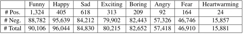
[image:6.595.89.511.62.121.2]# Neg. 88,782 95,639 84,212 79,902 82,443 57,326 46,746 15,857 # Total 90,106 96,044 84,830 80,215 82,652 57,418 46,910 15,881
Table 1: Amazon Mechanical Turk annotation label counts.
Funny Happy Sad Exciting Boring Angry Fear Heartwarming # Pos. 1,781 4,847 788 1,613 216 763 285 326 # Neg. 88,277 91,075 84,031 78,573 82,416 56,584 46,622 15,542 # Total1 90,058 95,922 84,819 80,186 82,632 57,347 46,907 15,868
Table 2: Ground truth annotation label counts for each emotion.2
tors do not expect the next one to be either. Due to these reasons, there is a lack of sufficient and high quality labeled data for emotion research. Some researchers have studied harnessing Twitter hash-tags to automatically create an emotion annotated dataset (Wang et al., 2012).
In order to evaluate our approach in real world scenarios, instead of creating a high quality anno-tated dataset and then introducing artificial noise, we followed the common practice of crowdsouc-ing, and collected emotion annotations through Amazon Mechanical Turk (AMT). This AMT an-notated dataset was used as the low quality dataset
ˆ
Din our evaluation. After that, the same dataset was annotated independently by a group of expert annotators to create the ground truth. We evaluate the proposed approach on two factors, the effec-tiveness of the models for emotion classification, and the improvement of annotation quality pro-vided by the active learning procedure. We first describe the AMT annotation and ground truth an-notation, and then discuss the baselines and exper-imental results.
Amazon Mechanical Turk Annotation: we posted the set of 100K tweets to the workers on AMT for emotion annotation. We defined a set of annotation guidelines, which specified rules and examples to help annotators determine when to tag a tweet with an emotion. We applied substantial quality control to our AMT workers to improve the initial quality of annotation following the common practice of crowdsourcing. Each tweet was anno-tated by at least two workers. We used a series of tests to identify bad workers. These tests include (1) identifying workers with poor pairwise agree-ment, (2) identifying workers with poor perfor-mance on English language annotation, (3) iden-tifying workers that were annotating at
unrealis-tic speeds, (4) identifying workers with near ran-dom annotation distributions, and (5) identifying workers that annotate each tweet for a given TV show the same (or nearly the same) way. We man-ually inspected any worker with low performance on any of these tests before we made a final deci-sion about using any of their annotations.
For further quality control, we also gathered ad-ditional annotations from adad-ditional workers for tweets where only one out of two workers iden-tified an emotion. After these quality control steps we defined minimum emotion annotation thresh-olds to determine and assign preliminary emo-tion labels to tweets. Note that some tweets were discarded as mixed examples for each emotion based upon thresholds for how many times they were tagged, and it resulted in different number of tweets in each emotion dataset. See Table 1 for the statistics of the annotations collected from AMT.
Ground Truth Annotation: After we obtained the annotated dataset from AMT, we posted the same dataset (without the labels) to a group of ex-pert annotators. The exex-perts followed the same an-notation guidelines, and each tweet was labeled by at least two experts. When there was a disagree-ment between two experts, they discussed to reach an agreement or gathered additional opinion from another expert to decide the label of a tweet. We used this annotated dataset as ground truth. See Table 2 for the statistics of the ground truth an-notations. Compared with the ground truth, many emotion bearing tweets were missed by the AMT annotators, despite the quality control we applied. It demonstrates the challenge of annotation by crowdsourcing. The imbalanced class distribution
1The total number of tweets is lower than the AMT dataset
because the experts removed some off-topic tweets.
2Expert annotators had a Kappa agreement score of 0.639
●● ●
● ●
● ● ●
●
●
0.36 0.40 0.44 0.48 0.52 0.56 0.60 0.64
0 4500 9000 13500 18000 22500 27000 Number of Instances Re−annotated
Macro−a
v
er
aged MAP
Method ● Spread SVM−TF SVM−Delta−IDF
(a) Macro-Averaged MAP
● ●
● ●
● ●
● ●
●
●
0.28 0.33 0.38 0.43 0.48 0.53 0.58
0 4500 9000 13500 18000 22500 27000 Number of Instances Re−annotated
Macro−a
v
er
aged F1 Score
Method ● Spread SVM−TF SVM−Delta−IDF
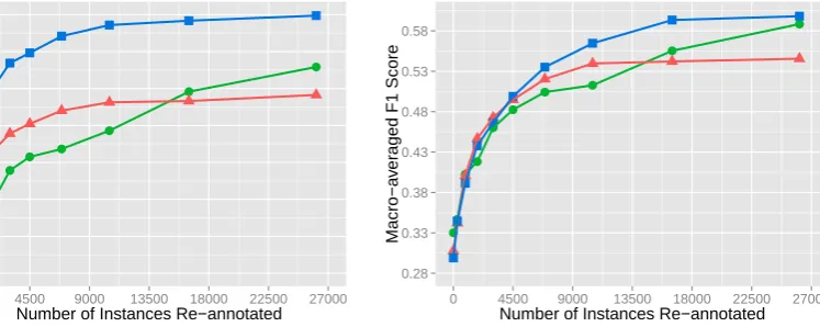
[image:7.595.126.500.62.211.2](b) Macro-Averaged F1 Score
Figure 1: Performance comparison of mislabeled instance selection methods. Classifiers become more accurate as more in-stances are re-annotated. Spread achieves comparable performance with SVMs in terms of both MAP and F1 Score.
aggravates the confirmation bias – the minority class examples are especially easy to miss when labeling quickly due to their rare presence in the dataset.
Evaluation Metric: We evaluated the results with both Mean Average Precision (MAP) and F1 Score. Average Precision (AP) is the average of the algorithm’s precision at every position in the confidence ranked list of results where a true emo-tional document has been identified. Thus, AP places extra emphasis on getting the front of the list correct. MAP is the mean of the average pre-cision scores for each ranked list. This is highly desirable for many practical application such as intelligent search, recommendation, and target ad-vertising where users almost never see results that are not at the top of the list. F1 is a widely-used measure of classification accuracy.
Methods: We evaluated the overall perfor-mance relative to the common SVM bag of words approach that can be ubiquitously found in text mining literature. We implemented the following four classification methods:
• Delta-IDF: Takes the dot product of the Delta IDF weight vector (Formula 1) with the document’s term frequency vector.
• Spread: Takes the dot product of the distri-bution spread weight vector (Formula 3) with the document’s term frequency vector. For all the experiments, we used spread parame-ters= 2.
• SVM-TF: Uses a bag of words SVM with term frequency weights.
• SVM-Delta-IDF: Uses a bag of words SVM classification with TF.Delta-IDF weights (Formula 2) in the feature vectors before training or testing an SVM.
We employed each method to build the active learner C described in Algorithm 1. We used standard bag of unigram and bigram words rep-resentation andtopic-based fold cross validation. Since in real world applications people are primar-ily concerned with how well the algorithm will work for new TV shows or movies that may not be included in the training data, we defined a test fold for each TV show or movie in our labeled data set. Each test fold corresponded to a training fold containing all the labeled data from all the other TV shows and movies. We call it topic-based fold cross validation.
We built the SVM classifiers using LIB-LINEAR (Fan et al., 2008) and applied its L2-regularized support vector regression model. Based on the dot product or SVM regression scores, we ranked the tweets by how strongly they express the emotion. We selected the topmtweets with the highest dot product or regression scores but conflicting preliminary AMT labels as the sus-pected mislabeled instances for re-annotation, just as described in Algorithm 1. For the experimental purpose, the re-annotation was done by assigning the ground truth labels to the selected instances. Since the dataset is highly imbalanced, we ap-plied the under-sampling strategy when training the classifiers.
re-annotated. The X axis shows the total number of data points that have been examined for each emotion so far till the current iteration (i.e., 300, 900, 1800, 3000, 4500, 6900, 10500, 16500, and 26100). We reported both the macro-averaged MAP (Figure 1a) and the macro-averaged F1 Score (Figure 1b) on eight emotions as the over-all performance of three competitive methods – Spread, SVM-Delta-IDF and SVM-TF. We have also conducted experiments using Delta-IDF, but its performance is low and not comparable with the other three methods.
Generally, Figure 1 shows consistent perfor-mance gains as more labels are corrected during active learning. In comparison, SVM-Delta-IDF significantly outperforms SVM-TF with respect to both MAP and F1 Score. SVM-TF achieves higher MAP and F1 Score than Spread at the first few iterations, but then it is beat by Spread after 16,500 tweets had been selected and re-annotated till the eighth iteration. Overall, at the end of the active learning process, Spread outperforms SVM-TF by 3.03% the MAP score (and by 4.29% the F1 score), and Delta-IDF outperforms SVM-TF by 8.59% the MAP score (and by 5.26% the F1 score). Spread achieves a F1 Score of 58.84%, which is quite competitive compared to 59.82% achieved by IDF, though SVM-Delta-IDF outperforms Spread with respect to MAP.
Spread and Delta-IDF are superior with respect to the time efficiency. Figure 2 shows the average training time of the four methods on eight emo-tions. The time spent training SVM-TF classi-fiers is twice that of SVM-Delta-IDF classiclassi-fiers, 12 times that of Spread classifiers, and 31 times that of Delta-IDF classifiers. In our experiments, on average, it took258.8seconds to train a SVM-TF classifier for one emotion. In comparison, the average training time of a Spread classifier was only 21.4seconds, and it required almost no pa-rameter tuning. In total, our method Spread saved up to (258.8−21.4)∗9∗8 = 17092.8 seconds (4.75hours) over nine iterations of active learning for all the eight emotions. This is enough time to re-annotate thousands of data points.
The other important quantity to measure is an-notation quality. One measure of improvement for annotation quality is the number of mislabeled in-stances that can be fixed after a certain number of active learning iterations. Better methods can fix more labels with fewer iterations.
0 100 200
Delta−IDF Spread SVM−Delta−IDF SVM−TF Method
A
v
er
age T
[image:8.595.314.506.59.220.2]raming Time (s)
Figure 2: Average training time on eight emotions. Spread re-quires only one-twelfth of the time spent to training an SVM-TF classifier. Note that the time spent tuning the SVM’s pa-rameters has not been included, but is considerable. Com-pared with such computationally expensive methods, Spread is more appropriate for use with active learning.
● ●●
●● ●
● ●
●
●
0% 10% 20% 30% 40% 50% 60% 70% 80% 90% 100%
0 4500 9000 13500 18000 22500 27000 Number of Instances Re−annotated
P
ercentage of Fix
ed Labels
Method
● Spread SVM−TF SVM−Delta−IDF
Delta−IDF Random
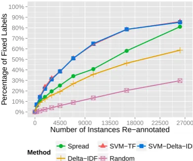
Figure 3: Accumulated average percentage of fixed labels on eight emotions. Spreading the feature weights reduces the number of data points that must be examined in order to cor-rect the mislabeled instances. SVMs require slightly fewer points but take far longer to build.
Besides the four methods, we also implemented a random baseline (Random) which randomly se-lected the specified number of instances for re-annotation in each round. We compared the im-proved dataset with the final ground truth at the end of each round to monitor the progress. Figure 3 reports the accumulated average percentage of corrected labels on all emotions in each iteration of the active learning process.
[image:8.595.308.504.298.461.2]6 Conclusion
In this paper, we explored an active learning ap-proach to improve data annotation quality for classification tasks. Instead of training the ac-tive learner using computationally expensive tech-niques (e.g., SVM-TF), we used a novel non-linear distribution spreading algorithm. This algorithm first weighs the features using the Delta-IDF tech-nique, and then non-linearly spreads out the distri-bution of the feature scores to enhance the model’s ability to discriminate at the feature level. The evaluation shows that our algorithm has the fol-lowing advantages: (1) It intelligently ordered the data points for annotators to annotate the most likely errors first. The accuracy was at least com-parable with computationally expensive baselines (e.g. SVM-TF). (2) The algorithm trained and ran much faster than SVM-TF, allowing annotators to finish more annotations than competitors. (3) The annotation process improved the dataset quality by positively impacting the accuracy of classifiers that were built upon it.
References
Carla E Brodley and Mark A Friedl. 1999. Identifying mislabeled training data. Journal of Artificial Intel-ligence Research, 11:131–167.
Chris Callison-Burch. 2009. Fast, cheap, and cre-ative: evaluating translation quality using amazon’s mechanical turk. InProceedings of EMNLP, pages 286–295. ACL.
Paul Ekman. 1999. Basic emotions. Handbook of cog-nition and emotion, 4:5–60.
Rong-En Fan, Kai-Wei Chang, Cho-Jui Hsieh, Xiang-Rui Wang, and Chih-Jen Lin. 2008. Liblinear: A library for large linear classification. The Journal of Machine Learning Research, 9:1871–1874.
Donghai Guan, Weiwei Yuan, Young-Koo Lee, and Sungyoung Lee. 2011. Identifying mislabeled train-ing data with the aid of unlabeled data. Applied In-telligence, 35(3):345–358.
Wenxin Jiang. 2001. Some theoretical aspects of boosting in the presence of noisy data. In Proceed-ings of ICML. Citeseer.
Adam Tauman Kalaia and Rocco A Servediob. 2005. Boosting in the presence of noise. Journal of Com-puter and System Sciences, 71:266–290.
Amitava Karmaker and Stephen Kwek. 2006. A boosting approach to remove class label noise. In-ternational Journal of Hybrid Intelligent Systems, 3(3):169–177.
Aniket Kittur, Ed H Chi, and Bongwon Suh. 2008. Crowdsourcing user studies with mechanical turk. InProceedings of CHI, pages 453–456. ACM.
Srivatsan Laxman, Sushil Mittal, and Ramarathnam Venkatesan. 2013. Error correction in learning us-ing svms. arXiv preprint arXiv:1301.2012.
Justin Martineau and Tim Finin. 2009. Delta tfidf: An improved feature space for sentiment analysis. In Proceedings of ICWSM.
John Mingers. 1989. An empirical comparison of pruning methods for decision tree induction. Ma-chine learning, 4(2):227–243.
Fabrice Muhlenbach, St´ephane Lallich, and Djamel A Zighed. 2004. Identifying and handling mislabelled instances. Journal of Intelligent Information Sys-tems, 22(1):89–109.
Robert Plutchik. 2001. The nature of emotions. Amer-ican Scientist, 89(4):344–350.
Umaa Rebbapragada, Carla E Brodley, Damien Sulla-Menashe, and Mark A Friedl. 2012. Active label correction. InProceedings of ICDM, pages 1080– 1085. IEEE.
James A Russell and Lisa Feldman Barrett. 1999. Core affect, prototypical emotional episodes, and other things called emotion: dissecting the elephant. Jour-nal of persoJour-nality and social psychology, 76(5):805. Burr Settles. 2010. Active learning literature sur-vey. Technical Report 1648, University of Wiscon-sin, Madison.
Victor S Sheng, Foster Provost, and Panagiotis G Ipeirotis. 2008. Get another label? improving data quality and data mining using multiple, noisy label-ers. InProceedings of KDD, pages 614–622. ACM. Rion Snow, Brendan O’Connor, Daniel Jurafsky, and Andrew Y Ng. 2008. Cheap and fast—but is it good?: evaluating non-expert annotations for natu-ral language tasks. InProceedings of EMNLP, pages 254–263.
Qi Su, Dmitry Pavlov, Jyh-Herng Chow, and Wendell C Baker. 2007. Internet-scale collection of human-reviewed data. InProceedings of WWW, pages 231– 240. ACM.
P Vannoorenberghe and T Denoeux. 2002. Handling uncertain labels in multiclass problems using belief decision trees. InProceedings of IPMU, volume 3, pages 1919–1926.
Sofie Verbaeten and Anneleen Van Assche. 2003. En-semble methods for noise elimination in classifica-tion problems. InMultiple classifier systems, pages 317–325. Springer.
Wenbo Wang, Lu Chen, Krishnaprasad Thirunarayan, and Amit P Sheth. 2012. Harnessing twitter” big data” for automatic emotion identification. In Pro-ceedings of SocialCom, pages 587–592. IEEE. Xinchuan Zeng and Tony R Martinez. 2001. An
al-gorithm for correcting mislabeled data. Intelligent data analysis, 5(6):491–502.