A Power Booster Factor for Out of Sample Tests of Predictability

Munich Personal RePEc Archive

A Power Booster Factor for

Out-of-Sample Tests of Predictability

Pincheira, Pablo

School of Business, Adolfo Ibáñez University

February 2017

Online at

https://mpra.ub.uni-muenchen.de/77027/

A Power Booster Factor for Out-of-Sample Tests of Predictability

Pablo M. Pincheira

School of Business, Adolfo Ibáñez University February 2017

Abstract

In this paper we introduce a “power booster factor” for out-of-sample tests of predictability. The relevant econometric environment is one in which the econometrician wants to compare the population Mean Squared Prediction Errors (MSPE) of two models: one big nesting model, and another smaller nested model. Although our factor can be used to improve the power of many out-of-sample tests of predictability, in this paper we focus on boosting the power of the widely used test developed by Clark and West (2006, 2007). Our new test multiplies the Clark and West t-statistic by a factor that should be close to one under the null hypothesis that the short nested model is the true model, but that should be greater than one under the alternative hypothesis that the big nesting model is more adequate. We use Monte Carlo simulations to explore the size and power of our approach. Our simulations reveal that the new test is well sized and powerful. In particular, it tends to be less undersized and more powerful than the test by Clark and West (2006, 2007). Although most of the gains in power are associated to size improvements, we also obtain gains in size-adjusted power. Finally we present an empirical application in which more rejections of the null hypothesis are obtained with our new test.

JEL Codes: C22, C52, C53, C58, E17, E27, E37, E47, F37.

Key Words: Time-series, forecasting, inference, inflation, exchange rates, random walk, out-of-sample.

Pincheira: Diagonal Las Torres 2640, Peñalolén, Santiago, Chile, [email protected].

1

1.

Introduction

In this paper we introduce a “power-booster-factor” for out-of-sample tests of predictability. The relevant econometric environment is one in which the econometrician wants to test for the difference between the population Mean Squared Prediction Errors (MSPE) of two models: one big nesting model, and another smaller nested model. The standard application of such comparisons is found in the exchange rate literature, where an economic model is used to generate forecasts that are compared to forecasts coming from the simple random walk.

Our “power-booster-factor” can be used to improve the power of many out-of-sample tests of predictability. Yet, in this paper, we focus on boosting the power of the widely used test developed by Clark and West (2006, 2007) (hereafter CW). We construct a new test multiplying the CW t-statistic by our “power-booster-factor”.

The key idea relies on the fact that this factor should be close to one under the null hypothesis that the short nested model is correct, but should be greater than one under the alternative hypothesis that the big nesting model is more adequate. This new test displays two interesting features. First, standard normal critical values seem to work well, meaning that the test is correctly sized, and second, the test is relatively powerful when compared to the widely used CW test.

Out-of-sample analyses have become fairly usual in time series econometrics to compare either different forecasting methods or the adequacy of economic models. Accordingly, during the last two decades several papers have proposed different out-of-sample testing strategies. For instance, Diebold and Mariano (1995) and West (1996) are leading articles in this literature.

When the objective is to compare population MSPE of two models, and one of them is nested in the other, a vast literature has documented that the traditional methods proposed by Diebold and Mariano (1995) and West (1996) are inadequate, see for instance West (1996, 2006). In particular McCracken (2007) derives the correct asymptotic distribution of traditional comparisons of MSPE between nested models concluding that, in general, usual tests are not normal. Moreover, McCracken (2007) provides the asymptotic distribution of four widely used statistics to compare population MSPE in nested environments. The extension to direct multistep ahead forecasts is made in Clark and McCracken (2005). In general terms the tests follow a non-standard distribution.

An alternative approach is presented by CW, who show that the asymptotic distribution of a simple encompassing t-statistic is well approximated by a standard normal distribution under the null hypothesis. In the particular case in which the null model posits a martingale process for the predictand, CW shows that the correct asymptotic distribution is indeed standard normal.

2

number of observations for parameter estimation. This problem is typically associated to low power of out-of sample tests, see for instance Inoue and Kilian (2013). In addition, in many relevant applications it is possible to think that the relevant alternative and null models are relatively close to each other. For instance, given that in relatively efficient asset markets we should expect little or no predictability of returns, it is critical to rely on high power tests, so they can detect this presumably little evidence against the null hypothesis.

The joint use of the CW test and our “power-booster-factor” allows us to propose a new test with relatively high power based on asymptotically normal critical values, which are very simple to use.

We use Monte Carlo simulations to explore the size, power and size-adjusted-power of our new test when forecasting one-step-ahead. We are interested in its performance both absolutely and relative to CW, which is the other usual asymptotically normal test used in nested environments. In our simulations, we calibrate our parameters and sample sizes to macro applications based on monthly exchange rates or monthly CPI inflation.

Simulation results reveal that our new test behaves as expected: it is, in general, correctly sized and more powerful than CW. We notice, however, that improvements in size-adjusted-power are moderate, and gains in power are mostly induced by the reduction in size distortions traditionally reported in CW.

While our test may display adequate size and high power, there are plenty of subtleties that deserve mentioning: First, our test tends to be slightly undersized when carrying out inference at the 10% level, but it is a little oversized at the 1% level. Second, in applied work the researcher needs to make a decision about one free parameter. We provide some suggestions on how to pick that parameter, but more should be done in the future.

We emphasize that we are testing equal population forecasting ability. In other words we use forecast comparisons as a model evaluation technique. We leave as an extension for future research the connection of our test with procedures to obtain good forecasts on a given sample. See Giacomini and White (2006) for an interesting discussion about the differences in evaluating forecasting methods and models.

The rest of the paper is organized as follows. Section 2 outlines the general econometric environment, the CW test, the “power-booster-factor” and the construction of our new test. Section 3 shows some asymptotic and finite sample results and observations. In section 4 we describe our DGPs and the simulation setup. Results of the Monte Carlo experiment are shown in section 5. Section 6 illustrates the use of our test in an empirical application and section 7 concludes.

2.

Econometric Setup and Forecast Evaluation Framework

2.1 Basic Econometric Setup

3

(2.1) = β + (model 1: null model),

(2.2) = β + γ+ (model 2: alternative model),

where e1t+1 and e2t+1 are zero mean martingale difference sequences meaning that E(eit+1|Ft)=0 for i=1,2. Here Ft

represents the sigma-field generated by current and past values of Xt, Zt andeit for i=1,2.

We are interested in evaluating the following null hypothesis: H0: γ=0. When this hypothesis is true, model 2

and model 1 are the same. This means that in population, forecasts, forecast errors and Mean Squared Prediction Errors (MSPE) are the same in both models. Under the alternative, γ≠0, and forecasts will be different in both models. In particular, since model 2 includes relevant information for explaining yt, the population forecasts

from model 2 will be superior to those of model 1, meaning that model 2 will have a lower MSPE than model 1.

We focus on the evaluation of our proposed test when comparing one-step-ahead forecasts. Let _{, |} and

, | represent h period ahead forecasts from each of the two models. Let β be a least squares estimate of model 1 that only uses data up to period t, with β and the model 2 counterparts. Then one-step-ahead forecasts and forecasts errors are given by the following expressions

(2.3) _{, |} = β , _{, |} = β + .

(2.4) ̂ _{, |} ≡ - β , ̂ _{, |} ≡ - β -

2.2 The test by Clark and West

As our “power-booster-factor” is heavily based on the CW test, it will be useful to explain in some detail the rationale behind this widely used test. To that end we need to describe our out-of-sample exercises. Let us assume that we have a total of T+1 observations on . The end point of the first sample used to estimate regression parameters is observation R. We generate a sequence of P one-step-ahead forecasts estimating the models in either rolling windows of fixed size R or recursive windows of size equal or greater than R.

For rolling windows, to generate the first set of forecasts we estimate our models with the first R observations of our sample. Thus, these forecasts are built with information available only at time R and are compared to the observation . Next, we estimate our models with the second rolling window of size R that includes observations 2 through R+1. These forecasts are compared to observation . We continue until the last forecasts are built using the last R available observations for estimation. These forecasts are compared to observation .

4

size grows with the number of available observations for estimation. For instance, the first forecast is constructed estimating the models in a window of size R, whereas the final forecast is constructed based on models estimated in a window of size T. Thus, we generate a total of P forecasts, with P satisfying R+(P-1)+1=T+1. So P=T+1-R.

Sample estimates of Mean Squared Prediction Errors (MSPE) from the two models are

2.5 = 1 ̂ , | !"

#

2.6 = 1 ̂ , | . !"

#

Under the null, the population MSPE of both models is the same: = ; under the alternative, the population MSPE of the bigger model should be lower than the population MSPE of the smaller model: > . Specifically, construction of CW begins by producing an adjusted estimate for the MSPE from model 21,

2.7 − '(). = 1 [ ̂ , | − + , | − , | , ]. !"

#

Now define . to be a consistent estimate of the long run variance of ̂ _{, |} − [ ̂ _{, |} − + _{, |} −

, | , ]. The CW test relies on the following t-statistic

2.8 − − '(). 0.

Notice that

2.9 ̂ _{, |} = + − _{, |} , =+ − _{, |} + _{, |} − _{, |} ,

Therefore

2.10 [ ̂ _{, |} − + , | − , | , ] = [ ̂ , | + 2 ̂ , | + , | − , | ,]

Or, equivalently,

2.11 [ ̂ _{, |} − + , | − , | , ] = [ ̂ , | − 2 ̂ , | + ̂ , | − ̂ , | ,]

Consequently, (2.7) could also be written as follows

5

2.12 − '(). = 1 [ ̂ , | − 2 ̂ , | + ̂ , | − ̂ , | ,] !"

#

From (2.12) it is straightforward to see that the numerator of the CW t-statistic is equal to

2.13 2 ̂ , | + ̂ , | − ̂ , | , !"

#

.

2.3The power-booster-factor

Let us consider the following term

2.14 2 − − '() =1 ∑#!" [ ̂ , | + 2 ̂ , | + ̂ , | − ̂ , | ,] 1 ∑ !" ̂ _{, |}

#

Notice that the numerator in (2.14) corresponds to plus the CW core statistic. This is important, because this last statistic has a different behavior under the null and alternative hypotheses. When the null hypothesis is true, we expect the core CW statistic to be close to zero, therefore, under the null

2.15 2 − − '() ≈1 ∑ #!" ̂ , | 1 ∑ !" ̂ _{, |}

#

= 1

Under the alternative, the core CW statistic should be positive, which implies

2.16 2 − − '() =1 ∑ #!" [ ̂ , | + 2 ̂ , | + ̂ , | − ̂ , | ,] 1 ∑ !" ̂ _{, |}

#

> 1

Under standard assumptions in the literature, expression (2.14) will converge in probability to 1 when the null hypothesis is true. We will see this with formal arguments in section 3.

It is important to notice, however, that there is no mathematical way to guarantee a positive numerator in (2.14). This, in addition to our desire of making the factor (2.14) even bigger under the alternative hypothesis, lead us to raise expression (2.14) to some positive and even scalar λ_{as follows}

2.17 8 2 − − '() 9:= ;1 ∑#!" [ ̂ , | + 2 ̂ , | + ̂ , | − ̂ , | ,] 1 ∑ !" ̂ _{, |}

#

<

6

Expression (2.17) introduces our “power booster factor”. It depends on the parameter λ, which should play no role asymptotically under the null hypothesis. We will explore via simulations the different behavior of our “power booster factor” as a function of λ in section 5.

2.4Our New Test

We propose to multiply the CW t-statistic by the factor in (2.17) to construct an asymptotically normal test. As we will see in the next section, under standard assumptions in the literature, expression (2.17) will converge in probability to 1 when the null hypothesis is true. This, Slutsky’s theorem plus asymptotic normality of the test by Clark and West (2006) ensures asymptotic normality for our approach. In the case of the test in Clark and West (2007) which is not normal, we rely on the good behavior of the normal approximation described by simulations in that paper, and many others, to use normal critical values for our test as well.

We notice that under the null hypothesis both tests, ours and CW, should be asymptotically the same, but under the alternative hypothesis, the factor in (2.17) should be greater than 1, and therefore it should boost and improve the power of the CW test. Furthermore, the higher the CW core statistic is, the higher the factor in (2.17) is, which suggest that gains in power should be greater at the 5% level than at the 10% significance level, and also should be greater at the 1% than at the 5% significance level.

An alternative way to interpret our approach is to consider a different estimator of the long-run variance of

, | − [ , | − + , | − , | , ]. Let . be the estimator of this long-run variance appearing in the

denominator of (2.8). Our approach reduces to propose the following new variance estimator

2.18 . = 8 2 − − '() 9

" :

.

Therefore our new test could be written as follows

2.19 − − '(). 0.

Under the null hypothesis, the denominator in (2.19) should be close to 0. but under the alternative, it should be lower than 0. , which produces a higher t-statistic. Under standard assumptions in the literature consistency of

7

3.

Asymptotic and finite sample behavior of our approach

3.1 Simple asymptotic theory

Here we provide a formal asymptotic analysis for our new test in the particular case in which the null model is a simple martingale in difference process, as in Clark and West (2006). This means that in (2.1) and (2.2) we are considering the special case β=0. So the models are

(3.1) = ,

(3.2) = γ+

Under the null, γ=0, so in population the subscripts 1 and 2 are no longer necessary. Therefore we could write

(3.3) = ,

In (3.2), let denote an estimate of γ that relies on data going from either t-R+1 to t (rolling samples) or from 1 to t (recursive samples).2 We have

(3.4) _{, |} = 0, ̂ _{, |} = , ̂ _{, |} = - ,

(3.5) ̂ _{, |} - ̂ _{, |} = – ( - )2 = 2 − .

Thus the numerator of the CW statistic is

3.6 − − '(). =2

!"

#

And our “power booster factor” factor from (2.17) looks as follows:

3.7 8 2 − − '() 9

:

= ;1 ∑ #!" [ + 2 ] 1 ∑ !"

#

<

:

Under the null hypothesis, since yt+1 = et+1 is a martingale difference sequence, and , rely only on data that

ends in t, = = = = 0. Thus the expectation of the numerator of the CW statistic is

3.8 = − − '(). = 0.

8

Given that is also a martingale difference sequence we could use a standard central limit theorem for martingale processes to show asymptotic normality for the CW statistic. We need some additional assumptions to show that the “power booster factor” converges in probability to 1 under the null hypothesis.

Let us consider the following assumptions:

(3.9) = > 0 '>( lim_{!→C !} ∑_#!" = = .∗> 0 (3.10) =| | E < G < +∞ for ( > 1 for all t

(3.11) _! ∑_#!" !IJK .∗ as P goes to infinity

(3.12a) _! ∑_#!" !IJK L∗> 0 as P goes to infinity

(3.12b) M_! ∑ _#!" N" is bounded in probability

Assumptions (3.9), (3.10) and (3.11) are required for the central limit to hold true. See Hamilton (1994) for details. Therefore we have that

(3.13) √!_! ∑ _#!" → P 0, .∗

Similarly, assumption (3.10) implies that the law of large numbers holds for . Meaning that

(3.14) _! ∑ _#!" → 0

This convergence is achieved almost surely, and therefore it is also satisfied in probability. See White (2001) for further details.

Assumptions (3.12a) and (3.12b) are different alternatives required for our “power booster factor” to converge in probability to 1 under the null hypothesis. Assumption (3.12a) is more restrictive than (3.12b) because the sequence of the sample average of is required to converge in probability. Assumption (3.12b) does not require convergence. It requires the sample average of to be far away from zero, which is a reasonable requirement, given that this is the sample average of a sequence of positive random variables.

9

3.15 8 2 − − '() 9

:

= ;1 ∑#!" [ + 2 ] 1 ∑ !"

#

<

: !I

JK QL_L∗_∗R:= 1

We arrive at the same conclusion using assumption (3.11b) but writing (3.7) in a slightly different way:

3.16 8 2 − − '() 9:= ;1 ∑#!" [ + 2 ] 1 ∑ !"

#

<

:

= ;1 +1 ∑ #!" [2 ] 1 ∑ !"

#

<

:

The joint use of (3.14) and assumption (3.12b) implies that (3.16) converges in probability to 1 under the null hypothesis3.

Our proposal is to multiply the CW t-statistic by our “power booster factor”. Asymptotic normality under the null hypothesis follows from asymptotic normality of CW, the “power booster factor” converging to one in probability, plus the application of Slutsky’s theorem.

As usual in this literature, assumption (3.9) rules out the use of recursive or expanding windows in the out-of-sample analysis, so for asymptotic normality to hold true, we rely on rolling regressions.

As mentioned before, under the alternative hypothesis we expect the CW core statistic to be positive. This means a “power booster factor” greater than one.

3.17 8 2 − − '() 9

:

= ;1 +2 ∑#!" [ ] 1 ∑ !"

#

<

:

> 1

For one sided test, the implication is that our approach should have more power. To see this, we will use a notation similar to that in Clark and West (2007). In that paper the authors roughly write the following Normal approximation for the CW t-statistic:

3.18 √ S1 2 ̂ , | + ̂ , | − ̂ , | , − 2= ̂ , | + ̂ , | − ̂ , | , #

T ~VP 0, .∗

Where .∗ is 4 times the long run variance of ̂ _{, |} + ̂ _{, |} − ̂ _{, |} ,.

3_{Here we are using the following result: If Yn converges in probability to zero, and Xn is bounded in probability, then the product}

10

In what follows we will assume that the correct asymptotic distribution of the CW t-statistic is standard normal. Let us use more assumptions and notation. Let us define W, X_: , X_:∗, Y̅ and . as follows

3.19 _!∑ # 2 ̂ , | + ̂ , | − ̂ , | ,JK!IW ≡ 2= ̂ , | + ̂ , | − ̂ , | , as P goes to infinity

3.20 X: ≡ 8 2 − − '() 9 :

(3.21) !IJK ∗ > 0 as P goes to infinity

3.22 Plim_!→C X: ≡ X:∗= Q ∗_{+ W}

∗ R :

> 0

3.23 Y̅ ≡ 1 2 ̂ , |+ ̂ , | − ̂ , | , #

3.24 . > 0 ]^ ' _`>^]^a >a ^a]b'a`c `Y .∗_{> 0.}

We notice that in (3.19), (3.21), (3.22) and (3.24) we are assuming that the CW core statistic, ,

X: and . are convergent sequences in probability.

The normal approximation in (3.18) could be written as follows

3.25 √ [g̅ ! "h]_√i∗ ~VP 0,1

And by Slutsky’s theorem we have that

3.26 √ [g̅ ! "h]_{0i !} ~VP 0,1

We propose a test based on the multiplication of the CW t-statistic and our “power booster factor”. Assuming a standard normal asymptotic distribution for CW, using Slutsky’s theorem again and expression (3.22) we have

3.27 √ [g̅ ! "h]_{0i !} X: ~VP 0, X:∗

So, for large P, we expect the following approximation to work well

3.28 √!g̅ ! jk!

11 This means that for every L > 0

3.29 Pr 8 √ Y̅ X:

0. > L9 ≈ 1 n2o+X:∗,

p " 8q"√!hjk

∗_⁄√i∗

j_k∗ 9 r

(s

C

t

which implies

3.30 Pr Q √!g̅ ! jk!

0i ! > LR ≈√ uv "

w rxr(y

C

z {k∗"|√}√~∗

= 1 − Φ(_jt

k∗−

h√! √i∗)

where Φ corresponds to the standard normal cdf.

A similar analysis for the CW t-statistic leads to the following expression

3.31 Pr Q √!g̅ !_{0i !} > LR ≈_{√ u}vC "wrxr(y

t"|√}_√~∗ = 1 − Φ(L − h√! √i∗)

Substracting (3.31) from (3.30) we arrive to

3.32 Pr Q √!g̅ ! jk!

0i ! > LR − Pr Q √!g̅ !

0i ! > LR ≈ Φ(L − h√! √i∗)−Φ(_jt

k∗−

h√! √i∗)

From (3.32) we can get some asymptotic implications for both size and power. First, if under the null hypothesis

W = 0 we will also have X_:∗= 1, so our test statistic will have a standard normal distribution under the null. This implies that CW and our approach will have the same size. Second, if under the alternative hypothesis W > 0 we will also have X_:∗> 1. In expression (3.32) and for positive L, this means a reduction in the ratio τ/X_:∗ which will induce higher power when compared to the CW case. It is due to this property that we call our factor a “power booster factor”. Expression (3.32) is also useful to provide some intuition about the role of the λ

parameter. Under the alternative hypothesis we expect X_:∗ to be an increasing function of λ, which implies that the power of our test is also an increasing function of this parameter.

12

out-of-sample exercise (rolling, recursive or fixed). In the second paper, Clark and McCracken (2005) provide a generalization of their results for multistep ahead forecasts. Unfortunately, the resulting asymptotic distribution of the CW statistic is again a functional of Brownian motions but now depending on nuisance parameters. Differing from the previous work of Clark and McCracken (2001, 2005), one of the key contributions of CW is to show via simulations that normal critical values are indeed adequate in a variety of settings. They show that the cost of approximating the correct critical values by standard normal ones is in general low: it produces a little undersized test. Furthermore, simulations completed by Clark and McCracken (2013) and Pincheira and West (2016) are consistent with the view that the CW statistic can reasonably be thought of as approximately normal. We will see in the following sections that our approach also seems to work well with standard normal critical values in a variety of settings.

3.2 Finite sample behavior

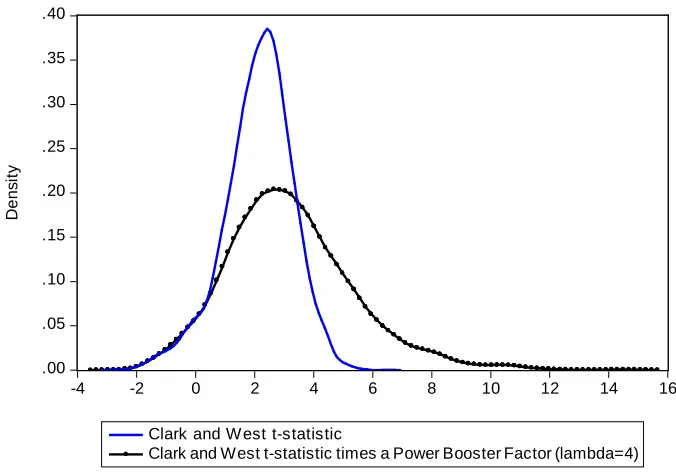
In finite samples of size typically available in macroeconomics, it is not always the case that the asymptotic theory will be useful to explain the behavior of our test. In particular, when the number of forecasts P is moderate or small, the multiplication of our “power booster factor” and the CW t-statistic has a skewed distribution: it tends to have a heavier right tail. See Figures 1-2 below. This is due to the fact that our test is a nonlinear function of the CW core statistic: When this core statistic is close to zero, our test is close to CW, but when the CW core statistic is large; our test would be even larger. This feature has implications in terms of size and power. In terms of power, the implication is that we expect our test to show more power relative to CW at the 1% significance level than at the 5% significance level. Similarly, our test should show more power relative to CW at the 5% level than at the 10% level. In terms of size, the same nonlinear dynamics holds true, so our test should display higher size than CW. This seems not to be a serious problem given that simulations completed in CW (2006, 2007) show that CW is a little undersized in finite samples. An increment in size could be beneficial if this increment is just moderate.

A final point reflects the observation that the “power booster factor” is an increasing function of the parameter λ_.

13

Figure 1: Kernel Densities of the Clark and West t-statistic and our New Test Distributions under the Null Hypothesis

.0 .1 .2 .3 .4 .5

-4 -3 -2 -1 0 1 2 3 4 5 6

Clark and W est t-statistic

Clark and W est t-statistic times a Power Booster Factor (lambda = 4)

De

n

s

it

y

Notes: Data for Figures 1 and 2 come from 5000 replications of DGP 3, using the recursive scheme with

parameters P=120 and λ=4. See section 4 next for a description of our Monte Carlo simulations.

Figure 2: Kernel Densities of the Clark and West t-statistic and our New Test Distributions under the Alternative Hypothesis

.00 .05 .10 .15 .20 .25 .30 .35 .40

-4 -2 0 2 4 6 8 10 12 14 16

Clark and W est t-statistic

Clark and West t-statistic times a Power Booster Factor (lambda=4)

D

e

n

s

it

y

14

4.

Monte Carlo Simulations

Our three simulation DGPs are stimulated by empirical work in asset pricing and macroeconomics. Most driving shocks are i.i.d. normal, but in DGP1 we also experiment with shocks displaying fat tails. In all simulations we consider both rolling and recursive samples, several values for the parameter λ _{in (2.17), a single value of the}

initial regression sample size R and four values of the number of one step ahead predictions P.

4.1 Experimental design

DGP 1: For the case where the null is a martingale model, we consider a DGP fairly similar to DGP 1 in Pincheira and West (2016). This DGP is such as the ones used in Clark and West (2006), Mankiw and Shapiro (1986), Nelson and Kim (1993), Stambaugh (1999), Campbell (2001), Tauchen (2001) and Pincheira (2013). This DGP is calibrated to match features of exchange rate series for which the martingale difference is a plausible null hypothesis and a model based on uncovered interest parity is a plausible alternative. The general setup is the following:

Null model:

4.1 = (model 1).

Alternative model:

4.2' = ۥ + c + (model 2),

4.2‚ c = €I + φ c + φ c" + ⋯ + φ…c" …" + y .

Here, both shocks, and y are independent white noise processes. While y is assumed to be Gaussian, is assumed to have a t(7) distribution displaying fat tails, which is a traditional feature of exchange rate returns. This simple setup maps into the notation of (2.1)-(2.2) via: the term β is absent and Zt

= (1 rt )′. In all our simulations, €• = €I = φ†= ⋯ = φ…= 0, so the process for c is a driftless AR(2)

model. Let

4.3 var = ˆ; var y = x; corr , y = Œ.

15

(4.4) φ φ ρ γ, under H0 γ under HA

DGP 1 1.19 -0.25 (1.75)2 (0.075)2 0 0 -1

In DGP 1, the null forecast (model 1) imposes €•=γ=0, thus assuming yt+1 = et+1. The null yields simply the

martingale difference or ‘‘no change’’ forecast of 0 for all t and all forecasting horizons. (In terms of the notation above, , | = 0 for all t.) In DGP 1, the alternative forecast (model 2) is obtained from equation (4.2a), i.e. from a regression of on the first lag of c and a constant. For the alternative, we compute forecasts using OLS estimates of our parameters, so they have the following shape

(4.5) | ۥ c .

Here, the t subscripts on the coefficients ۥ and emphasize that they are estimated from a sample that ends at date t.

The parameterization in DGP 1 is based roughly on estimates from the exchange rate application considered in the empirical work reported in Clark and West (2006), in which yt+1 is the monthly percentage change in a US

dollar bilateral exchange rate and rt is the corresponding interest differential. The parameters are obtained from

monthly data. For this DGP we consider an initial estimation window of 120 observations (R=120) and report results for several different number of predictions: P=120, 240, 360 and 1000. The initial window of R=120 corresponds to a sample size of 10 years, the values P=120, 240 and 360 represents 10, 20 and 30 years of predictions. We also consider the case in which P = 1000 to analyze the asymptotic behavior of our approach.

DGP 2: Our second DGP corresponds to the very same DGP 3 in Pincheira and West (2016). This DGP is motivated by the literature on commodity currencies. Our DGP 2 is calibrated to monthly returns of the Non-Fuel Commodity Price Index of the IMF, yt+1, and three commodity currencies versus the U.S. dollar: r1t =

Australia, r2t = South Africa and r3t = Chile. According to Chen, Rogoff and Rossi (2010) commodity currencies

should have the ability to predict commodity returns. Null model:

4.6 €• • (model 1).

Alternative model:

4.7a €_• c c _†c_† • (model 2),

4.7b c• €•I φ•c• y• , i=1,2,3.

16

4.8 €• = € I = € I = €†I= 0, • = 0.3, φ = φ = 0.33, φ†= 0.5 ; under H0 , γ1 = γ2 = γ3 = 0; under

HA, = −0.06 ; = -0.015; †=-0.06.

These parameters are calibrated to 1990-2015 monthly data, with the three currencies monthly average of daily values. The variance-covariance structure of the shocks ( _, y , y , y_† is given by 10-3times the following matrix

•

0.536 −0.296 −0.229 −0.221 −0.296 0.666 0.352 0.251 −0.229 0.352 1.09 0.251 −0.221 0.251 0.251 0.478

‘

We consider an initial estimation window of 120 observations (R=120) and several different number of predictions: P=85, 170, 340 and 1000.

DGP 3: Our last DGP is based on recent work exploring the predictive linkages between domestic and international inflation. Several articles analyze this relationship concluding that the linkage is important, both at the core and headline level, at least for some countries. See for instance Ciccarelli and Mojon (2010), Morales-Arias and Moura (2013), Hakkio (2009), Pincheira and Gatty (2016) and Medel, Pedersen and Pincheira (2016). For clarity, we relabel yt as o’“Iˆ and rt aso_a”••–, where CIIF stands for Core International Inflation Factor. The

DGP is as follows. Let et and νt be i.i.d. shocks.

(4.9) o’“Iˆ= €_o+ —_uo_a_`c + (model 1: null model), (4.10) o’“Iˆ= €_o+ —_oo’“Iˆ+ γ o˜™™š+γ o˜™™š_" + _a+1 (model 2: alternative model),

(4.11) o˜™™š= €_c+ —₁o˜™™š+—₂o˜™™š_" + y_a+1

We calibrate these two processes to match in-sample estimates for monthly core inflation for a sample of OECD countries. Parameters:

(4.12) €_u=0.15, —_u= 0.90, €_I = 0.05, — = 1.27, — = −0.3, _ˆ = 0.25 , _x = 0.1 ; corr( , y ) = 0.2; under H0, γ = γ₂= 0; under HA, γ =0.51, γ₂= −0.50.

In contrast to our previous DGPs, DGP 3 is highly persistent in all three expressions (4.9), (4.10) and (4.11). We consider an initial estimation window of 240 observations (R=240) and report results for several different number of predictions: P=120, 180, 240 and 1000. Differing also from our previous DGPs, now we do not impose the correct number of lags for o˜™™š in (4.10). We use BIC to choose the lag length with maximum lag

p=6, so in this DGP we deal with a certain degree of model uncertainty.

17

level for one sided tests. We construct estimates of the long run variance Vœ in (2.8) using Newey and West (1987, 1994).

5.

Simulation results

In this section we present simulation results for size, size-adjusted-power and raw power of our tests. To save space, complete results are only reported when the nominal size is 5%. Nevertheless, summary statistics for all three nominal sizes (10%, 5% and 1%) are also described in this section. Complete results for other relevant nominal sizes are in the appendix. We also report tables with the average across 5000 independent simulations of our “power booster factor”.

5.1 Simulation Results: Size.

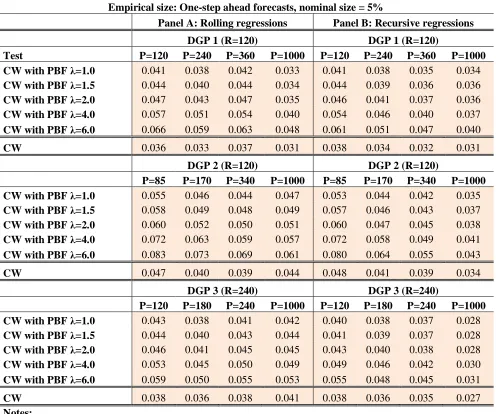
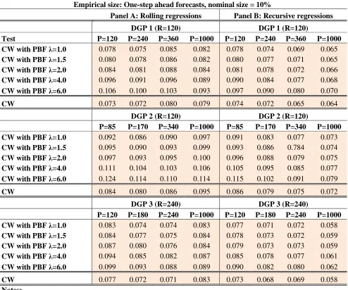
Results for nominal size 5% are in Table 1. From this table, in the rows labeled “CW” we see that the CW test is modestly undersized in all our DGPs and for all values of the number of forecasts P. This is also robust to the use of rolling and recursive windows. Table 6 indicates that the median size of CW is 0.037, below the nominal size of 0.05. Let us go back to Table 1. In the rows labeled “CW with PBF…” we present results for our approach. Three salient features are worth mentioning. First, empirical size is always higher than the equivalent figure for CW. Second, the empirical size of our approach is an increasing function of the parameter λ_{. Third; in}

Table 6 we see that the median size of our approach is 0.045, below the nominal size of 0.05. Nevertheless, our approach is not always undersized. In particular it is sometimes oversized for high values of λ. _{We notice,}

however, that in most entries of Table 1, results on size are better in our approach relative to CW. This means that size is higher than CW, but either below nominal size or slightly above it. This is particularly noticeable if we restrict ourselves to values of λ _{equal or below 2. In this case is only for DGP 2 and} P=85 that our approach is importantly oversized. This represents less than 10% of the relevant entries in Table 1. Other than that, our approach improves the empirical size of the CW test.

18

A slightly different picture is shown for nominal sizes of 1%. CW is still slightly undersized, but now, in most entries of Table A4 in the appendix, our approach is slightly oversized with a median of 0.011 (see Table 6). In most cases size distortions in our approach are modest, but in some cases for large values of λ_{, our approach is}

importantly oversized. Interestingly, for low values of λ (1 ≤ λ ≤ 2), the median size of our approach is 1%, and aside from the results of DGP 2 with P=85, our test seems to be, in most cases, correctly sized.

Table 1

Empirical size: One-step ahead forecasts, nominal size = 5%

Panel A: Rolling regressions Panel B: Recursive regressions

DGP 1 (R=120) DGP 1 (R=120)

Test P=120 P=240 P=360 P=1000 P=120 P=240 P=360 P=1000

CW with PBF λ_{=1.0 0.041 0.038 0.042 0.033 0.041 0.038 0.035 0.034}

CW with PBF λ_{=1.5 0.044 0.040 0.044 0.034 0.044 0.039 0.036 0.036}

CW with PBF λ_{=2.0 0.047 0.043 0.047 0.035 0.046 0.041 0.037 0.036}

CW with PBF λ_{=4.0 0.057 0.051 0.054 0.040 0.054 0.046 0.040 0.037}

CW with PBF λ_{=6.0 0.066 0.059 0.063 0.048 0.061 0.051 0.047 0.040}

CW 0.036 0.033 0.037 0.031 0.038 0.034 0.032 0.031

DGP 2 (R=120) DGP 2 (R=120)

P=85 P=170 P=340 P=1000 P=85 P=170 P=340 P=1000

CW with PBF λ_{=1.0 0.055 0.046 0.044 0.047 0.053 0.044 0.042 0.035}

CW with PBF λ_{=1.5 0.058 0.049 0.048 0.049 0.057 0.046 0.043 0.037}

CW with PBF λ_{=2.0 0.060 0.052 0.050 0.051 0.060 0.047 0.045 0.038}

CW with PBF λ_{=4.0 0.072 0.063 0.059 0.057 0.072 0.058 0.049 0.041}

CW with PBF λ_{=6.0 0.083 0.073 0.069 0.061 0.080 0.064 0.055 0.043}

CW 0.047 0.040 0.039 0.044 0.048 0.041 0.039 0.034

DGP 3 (R=240) DGP 3 (R=240)

P=120 P=180 P=240 P=1000 P=120 P=180 P=240 P=1000

CW with PBF λ_{=1.0 0.043 0.038 0.041 0.042 0.040 0.038 0.037 0.028}

CW with PBF λ_{=1.5 0.044 0.040 0.043 0.044 0.041 0.039 0.037 0.028}

CW with PBF λ_{=2.0 0.046 0.041 0.045 0.045 0.043 0.040 0.038 0.028}

CW with PBF λ_{=4.0 0.053 0.045 0.050 0.049 0.049 0.046 0.042 0.030}

CW with PBF λ_{=6.0 0.059 0.050 0.055 0.053 0.055 0.048 0.045 0.031}

CW 0.038 0.036 0.038 0.041 0.038 0.036 0.035 0.027

Notes:

19

2. In DGP 1 the null model posits that the predictand yt is white noise, the alternative that yt depends on a constant and a variable rt that

follows an autoregression of order 2. In DGPs 2 and 3, the null is that yt follows an AR(1), the alternative that yt is driven by additional

variables following autoregressive processes. This implies that the univariate process for yt is not an AR(1). Section 4 of the main body

of the paper gives exact specifications. In the exercises with DGP 1 and DGP 2 the alternative uses population lag lengths. In the exercises with DGP3 the alternative uses BIC to pick lags of the exogenous variable in the equation for yt . All three DGPs are estimated

by least squares.

3. Results are based on 5000 replications. A figure of 0.041 in the first column with numbers, for example, indicates that about 205 of the 5000 corresponding statistics were greater than 1.645, where 1.645 is the 5% critical value for a standard normal one-sided test.

4. Let R be the rolling sample size (left panel in Table 1) or the smallest recursive sample used to estimate parameters needed under the alternative to make a forecast (right panel in Table 1). Then R=120 in DGP 1 and DGP 2 and R=240 in DGP 3. Table 1 shows results for several different number of predictions P. In DGP 1 we consider P=120; P=240; P=360 and P=1000. In DGP 2 we consider P=85; P=170; P=340 and P=1000. In DGP 3 we consider P=120; P=180; P=240 and P=1000. Results for nominal sizes of 10% and 1%, are available in the Appendix.

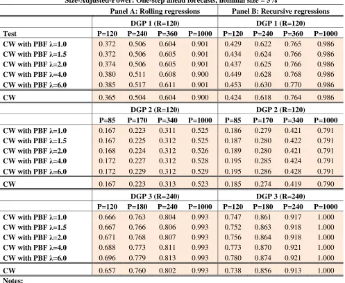
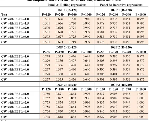
5.2 Simulation Results: Power. Table2 shows results for size-adjusted-power, Table 3 for power. Virtually all entries in Table 2 display higher size-adjusted-power for our approach relative to CW6. The only exception occurs for DGP 2, when P= 340 under the rolling scheme. In all other cases size-adjusted-power is higher when using our “power booster factor”. Differences are in general low, however. Table 6 shows the median size-adjusted-power for all three nominal sizes. The figures for CW are 0.741; 0.638 and 0.401 when nominal sizes are 10%, 5% and 1% respectively. The equivalent figures of our new approach are 0.745; 0.648 and 0.431. Consistent with our beliefs, gains in size-adjusted-power relative to CW are tiny when inference is carried out at the 10% level, small to moderate at the 5% level, and substantial when inference is carried out at the 1% level. Table 6 shows median results, but also consistent with our beliefs, Table 2 shows that size-adjusted-power is an increasing function of λ_{, so gains relative to CW are more important when} λ _{is high}. _{To give an example, Table}

2 indicates that for DGP 3, under the rolling scheme, when P=120, CW has a figure of size-adjusted-power equal to 0.657. For λ _{= 1, the equivalent figure of our approach is 0.666, only a tiny improvement relative to CW.}

Nevertheless, for λ _{= 6, our figure is 0.696, a considerable gain relative to CW. The same gains are less}

impressive at the 10% nominal size (see Table A2 in the appendix) but much more impressive when nominal size is 1%. In this case, the equivalent entries in Table A5 in the appendix show a figure for CW of 0.441. For our approach when λ _{= 6, our figure is 0.558. (See in Table A5 the case of DGP 3 under the rolling scheme,}

when P=120). A final point: gains in size-adjusted-power are more important for small and moderate values of the number of predictions P. Asymptotically, gains in size-adjusted-power tend to disappear.

20 Table 2

Size-Adjusted-Power: One-step ahead forecasts, nominal size = 5%

Panel A: Rolling regressions Panel B: Recursive regressions

DGP 1 (R=120) DGP 1 (R=120)

Test P=120 P=240 P=360 P=1000 P=120 P=240 P=360 P=1000

CW with PBF λ_{=1.0 0.372 0.506 0.604 0.901 0.429 0.622 0.765 0.986}

CW with PBF λ_{=1.5 0.372 0.506 0.605 0.901 0.434 0.624 0.766 0.986}

CW with PBF λ_{=2.0 0.374 0.506 0.605 0.901 0.437 0.625 0.766 0.986}

CW with PBF λ_{=4.0 0.380 0.511 0.608 0.900 0.449 0.628 0.768 0.986}

CW with PBF λ_{=6.0 0.385 0.517 0.611 0.901 0.453 0.630 0.770 0.986}

CW 0.365 0.504 0.604 0.900 0.424 0.618 0.764 0.986

DGP 2 (R=120) DGP 2 (R=120)

P=85 P=170 P=340 P=1000 P=85 P=170 P=340 P=1000

CW with PBF λ_{=1.0 0.167 0.223 0.311 0.525 0.186 0.279 0.421 0.791}

CW with PBF λ_{=1.5 0.167 0.225 0.312 0.525 0.187 0.280 0.422 0.791}

CW with PBF λ_{=2.0 0.168 0.224 0.312 0.526 0.189 0.280 0.421 0.791}

CW with PBF λ_{=4.0 0.172 0.227 0.312 0.528 0.195 0.285 0.424 0.791}

CW with PBF λ_{=6.0 0.172 0.229 0.312 0.529 0.195 0.286 0.428 0.791}

CW 0.167 0.223 0.313 0.523 0.185 0.274 0.419 0.790

DGP 3 (R=240) DGP 3 (R=240)

P=120 P=180 P=240 P=1000 P=120 P=180 P=240 P=1000

CW with PBF λ_{=1.0 0.666 0.763 0.804 0.993 0.747 0.861 0.917 1.000}

CW with PBF λ_{=1.5 0.667 0.766 0.806 0.993 0.752 0.863 0.918 1.000}

CW with PBF λ_{=2.0 0.671 0.768 0.807 0.993 0.756 0.864 0.918 1.000}

CW with PBF λ_{=4.0 0.688 0.773 0.811 0.993 0.773 0.870 0.921 1.000}

CW with PBF λ_{=6.0 0.696 0.779 0.813 0.993 0.780 0.874 0.921 1.000}

CW 0.657 0.760 0.802 0.993 0.738 0.856 0.913 1.000

Notes:

1. Table 2 displays figures on size-adjusted-power for two tests of equal population mean squared prediction errors (MSPEs) against the one-sided alternative that one model has higher accuracy (lower MSPE). Size-adjusted-power represents the percentage of correct rejections of the null hypothesis enforcing the empirical size of the tests to coincide with their nominal size. Rows with the label “CW” display results of the test proposed in Clark and West (2006, 2007). Rows with the label “CW with PBF…” display results of the test proposed in this paper. The term “PBF” stands for Power Booster Factor. Our test is the result of the multiplication of the t-statistic proposed in Clark and West (2006, 2007) and the Power Booster Factor presented in expression (2.17). This factor should be close to one under the null hypothesis, but should be greater than one under the alternative hypothesis. The implication is that our test should have more power than the test in Clark and West (2006, 2007). As the Power Booster Factor depends on the parameter λ_{, we present results}

for five different alternatives for this parameter: λ_=1; λ_=1.5; λ_=2; λ_{=4; and} λ=_6.

21

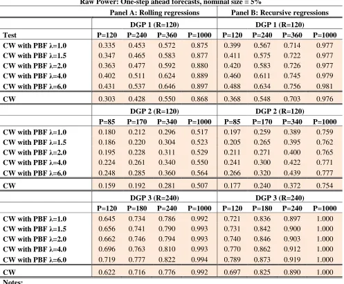
Table 3 shows result on raw power. Virtually all entries in Table 3 display higher power for our approach relative to CW7_{. The only exception occurs for DGP 3, when P= 1000 under the recursive scheme. In this case}

figures on power are all equal to one both in CW and our approach. In all other cases power is higher when using our “power booster factor”. Differing from our previous analysis on size-adjusted-power, now the gains of our approach relative to CW are, in general, substantial. Table 6 shows the median power for all three nominal sizes. The figures for CW are 0.702; 0.586 and 0.342 when nominal sizes are 10%, 5% and 1% respectively. The equivalent figures of our new approach are 0.731; 0.646 and 0.468. We notice that for CW median figures on power are lower than on size-adjusted-power, reflecting the fact that CW is a little undersized. When using our “power booster factor” we find mixed results. Figures on power are lower than on size-adjusted-power when inference is carried out at the 10% significance level, which is consistent with our approach being a little undersized. Nevertheless, figures on power are higher than on size-adjusted-power when inference is carried out at the 5% and 1% significance levels, which is consistent with our approach being a little oversized, especially for high values of λ, when the nominal size is set to 1%.

Gains in power relative to CW are moderate when inference is carried out at the 10% level, higher at the 5% level, and huge when inference is carried out at the 1% level. Table 3 also shows that power is an increasing function of λ_{, so gains relative to CW are more important when} λ _{is high}. _{To give an example, Table 3 indicates}

that for DGP 1, under the recursive scheme, when P=120, CW has a figure on power equal to 0.368. For λ _{= 1,}

the equivalent figure of our approach is 0.399, a small improvement relative to CW. Nevertheless, for λ _{= 6, our}

figure is 0.488, a substantial gain relative to CW. The same gains are slightly lower at the 10% nominal size (see Table A3 in the appendix) but much more impressive when nominal size is 1%. In this case, the equivalent entries in Table A6 in the appendix show a figure for CW of 0.147. For our approach when λ _{= 6, our figure is}

0.343. (See in Table A3 the case of DGP 1 under the recursive scheme, when P=120). Gains in power are more important for small and moderate values of the number of predictions P and tend to disappear as the number of predictions grows to infinity.

We notice that some of the gains in power come from comparing a slightly oversized test with a slightly undersized test. For instance, in rolling regressions for DGP 1, P=360 and λ=4, Table 1 shows a figure on size for our approach of 0.054. The same figure for CW is 0.037. Gains in power in this case are high. Table 3 shows that our approach has raw power equal to 62.4%. The equivalent figure for CW is 55%. Not all the gains in power come from comparing undersized to oversized tests. In many cases our approach generates a less undersized test than CW. This, plus some gains in size-adjusted-power, generate a test with higher raw power.

22 Table 3

Raw Power: One-step ahead forecasts, nominal size = 5%

Panel A: Rolling regressions Panel B: Recursive regressions

DGP 1 (R=120) DGP 1 (R=120)

Test P=120 P=240 P=360 P=1000 P=120 P=240 P=360 P=1000

CW with PBF λ_{=1.0 0.335 0.453 0.572 0.875 0.399 0.567 0.714 0.977}

CW with PBF λ_{=1.5 0.347 0.465 0.583 0.877 0.411 0.575 0.722 0.977}

CW with PBF λ_{=2.0 0.363 0.477 0.592 0.880 0.420 0.583 0.726 0.977}

CW with PBF λ_{=4.0 0.402 0.511 0.624 0.889 0.460 0.611 0.745 0.979}

CW with PBF λ_{=6.0 0.431 0.537 0.646 0.897 0.488 0.634 0.756 0.981}

CW 0.303 0.428 0.550 0.868 0.368 0.548 0.703 0.976

DGP 2 (R=120) DGP 2 (R=120)

P=85 P=170 P=340 P=1000 P=85 P=170 P=340 P=1000

CW with PBF λ_{=1.0 0.180 0.212 0.296 0.517 0.197 0.259 0.389 0.759}

CW with PBF λ_{=1.5 0.186 0.220 0.304 0.523 0.205 0.265 0.395 0.762}

CW with PBF λ_{=2.0 0.195 0.228 0.311 0.529 0.211 0.271 0.400 0.765}

CW with PBF λ_{=4.0 0.224 0.261 0.340 0.550 0.241 0.300 0.422 0.771}

CW with PBF λ_{=6.0 0.248 0.285 0.360 0.564 0.266 0.320 0.439 0.777}

CW 0.159 0.192 0.281 0.507 0.177 0.240 0.372 0.754

DGP 3 (R=240) DGP 3 (R=240)

P=120 P=180 P=240 P=1000 P=120 P=180 P=240 P=1000

CW with PBF λ_{=1.0 0.645 0.734 0.786 0.992 0.721 0.836 0.897 1.000}

CW with PBF λ_{=1.5 0.656 0.741 0.790 0.993 0.731 0.842 0.900 1.000}

CW with PBF λ_{=2.0 0.662 0.746 0.794 0.993 0.740 0.846 0.903 1.000}

CW with PBF λ_{=4.0 0.696 0.763 0.810 0.993 0.770 0.862 0.912 1.000}

CW with PBF λ_{=6.0 0.719 0.777 0.822 0.994 0.789 0.873 0.919 1.000}

CW 0.622 0.716 0.776 0.992 0.697 0.825 0.890 1.000

Notes:

1. Table 3 displays figures on power (also called raw power) for two tests of equal population mean squared prediction errors (MSPEs) against the one-sided alternative that one model has higher accuracy (lower MSPE). Power represents the percentage of correct rejections of the null hypothesis using standard normal critical values. Rows with the label “CW” display results of the test proposed in Clark and West (2006, 2007). Rows with the label “CW with PBF…” display results of the test proposed in this paper. The term “PBF” stands for Power Booster Factor. Our test is the result of the multiplication of the t-statistic proposed in Clark and West (2006, 2007) and the Power Booster Factor presented in expression (2.17). This factor should be close to one under the null hypothesis, but should be greater than one under the alternative hypothesis. The implication is that our test should have more power than the test in Clark and West (2006, 2007). As the Power Booster Factor depends on the parameter λ_{, we present results for five different alternatives for this parameter:} λ_=1; λ_=1.5; λ_=2; λ_{=4; and} λ=_6.

2. See notes to Table 1 for further details.

23

either 2 or 4, and for inference at the 1% significance level set λ to either 1, 1.5 or 2. This recommendation is based on the observation that the risk of obtaining an oversized test is higher at tighter significance levels.

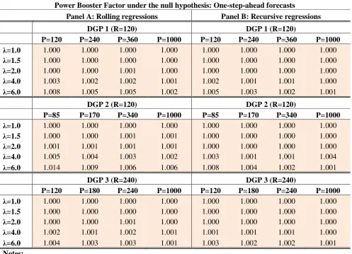
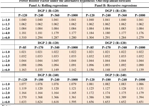
A final point: Tables 4 and 5 shows the average across our 5000 simulations of our “power booster factor” computed both under the null and alternative hypotheses. As expected, our factor is very close to one under the null, and greater than 1 under the alternative hypothesis. These figures are consistent with our results shown in previous tables, both on size and power.

Table 4

Power Booster Factor under the null hypothesis: One-step-ahead forecasts

Panel A: Rolling regressions Panel B: Recursive regressions

DGP 1 (R=120) DGP 1 (R=120)

P=120 P=240 P=360 P=1000 P=120 P=240 P=360 P=1000

λ_{=1.0 1.000 1.000 1.000 1.000 1.000 1.000 1.000 1.000}

λ_{=1.5 1.000 1.000 1.000 1.000 1.000 1.000 1.000 1.000}

λ_{=2.0 1.000 1.000 1.001 1.000 1.000 1.000 1.000 1.000}

λ_{=4.0 1.003 1.002 1.002 1.001 1.002 1.001 1.001 1.000}

λ_{=6.0 1.008 1.005 1.005 1.002 1.005 1.003 1.002 1.001}

DGP 2 (R=120) DGP 2 (R=120)

P=85 P=170 P=340 P=1000 P=85 P=170 P=340 P=1000

λ_{=1.0 1.000 1.000 1.000 1.000 1.000 1.000 1.000 1.000}

λ_{=1.5 1.000 1.000 1.001 1.001 1.000 1.000 1.000 1.000}

λ_{=2.0 1.001 1.001 1.001 1.001 1.000 1.000 1.000 1.000}

λ_{=4.0 1.005 1.004 1.003 1.002 1.003 1.001 1.001 1.004}

λ_{=6.0 1.014 1.009 1.006 1.006 1.008 1.004 1.002 1.001}

DGP 3 (R=240) DGP 3 (R=240)

P=120 P=180 P=240 P=1000 P=120 P=180 P=240 P=1000

λ_{=1.0 1.000 1.000 1.000 1.000 1.000 1.000 1.000 1.000}

λ_{=1.5 1.000 1.000 1.000 1.000 1.000 1.000 1.000 1.000}

λ_{=2.0 1.000 1.000 1.001 1.000 1.000 1.000 1.000 1.000}

λ_{=4.0 1.002 1.001 1.002 1.001 1.001 1.001 1.001 1.000}

λ_{=6.0 1.004 1.003 1.003 1.001 1.003 1.002 1.002 1.001}

Notes:

1. Table 4 displays the average of our Power Booster Factor presented in expression (2.17) across our 5000 replications when the null hypothesis is true in our three DGPs. This factor should be close to one under the null hypothesis, but should be greater than one under the alternative hypothesis.

2. See notes to Table 1 for further details.

24 Table 5

Power Booster Factor under the alternative hypothesis: One-step-ahead forecasts

Panel A: Rolling regressions Panel B: Recursive regressions

DGP 1 (R=120) DGP 1 (R=120)

P=120 P=240 P=360 P=1000 P=120 P=240 P=360 P=1000

λ_{=1.0 1.040 1.040 1.041 1.041 1.040 1.041 1.040 1.041}

λ_{=1.5 1.062 1.062 1.062 1.062 1.062 1.062 1.062 1.062}

λ_{=2.0 1.084 1.084 1.084 1.084 1.084 1.084 1.083 1.084}

λ_{=4.0 1.181 1.181 1.179 1.177 1.184 1.180 1.177 1.176}

λ_{=6.0 1.310 1.294 1.287 1.280 1.304 1.291 1.284 1.279}

DGP 2 (R=120) DGP 2 (R=120)

P=85 P=170 P=340 P=1000 P=85 P=170 P=340 P=1000

λ_{=1.0 1.021 1.021 1.022 1.022 1.021 1.021 1.022 1.022}

λ_{=1.5 1.032 1.033 1.033 1.033 1.032 1.032 1.033 1.032}

λ_{=2.0 1.044 1.044 1.045 1.044 1.044 1.044 1.044 1.044}

λ_{=4.0 1.098 1.096 1.094 1.091 1.096 1.093 1.092 1.090}

λ_{=6.0 1.163 1.155 1.149 1.142 1.156 1.148 1.145 1.139}

DGP 3 (R=240) DGP 3 (R=240)

P=120 P=180 P=240 P=1000 P=120 P=180 P=240 P=1000

λ_{=1.0 1.077 1.078 1.078 1.079 1.081 1.082 1.083 1.086}

λ_{=1.5 1.119 1.120 1.120 1.121 1.125 1.127 1.128 1.131}

λ_{=2.0 1.164 1.164 1.164 1.165 1.172 1.174 1.175 1.179}

λ_{=4.0 1.370 1.368 1.366 1.361 1.386 1.388 1.389 1.394}

λ_{=6.0 1.633 1.624 1.618 1.595 1.656 1.653 1.652 1.651}

Notes:

1. Table 5 displays the average of our Power Booster Factor presented in expression (2.17) across our 5000 replications when the alternative hypothesis is true in our three DGPs. This factor should be close to one under the null hypothesis, but should be greater than one under the alternative hypothesis.

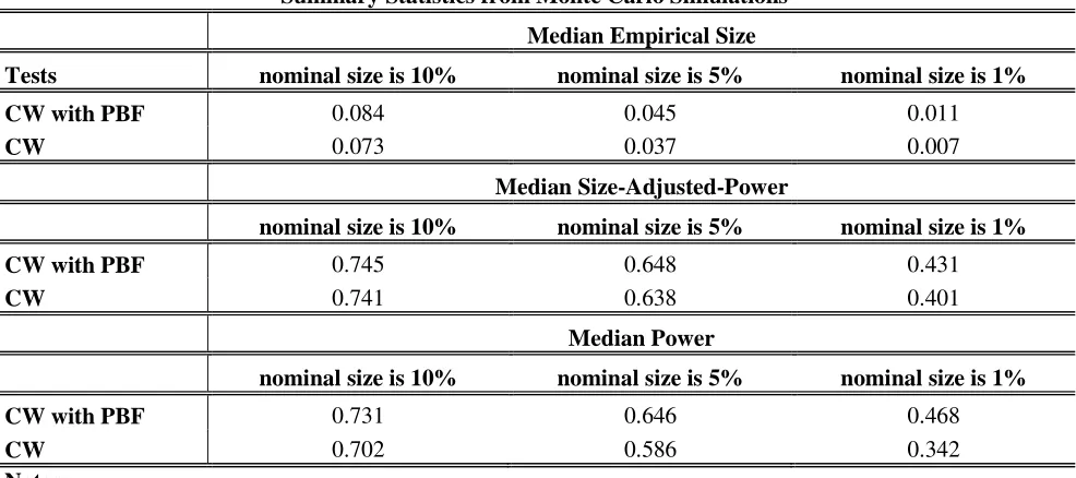
25 Table 6

Summary Statistics from Monte Carlo Simulations

Median Empirical Size

Tests nominal size is 10% nominal size is 5% nominal size is 1%

CW with PBF 0.084 0.045 0.011

CW 0.073 0.037 0.007

Median Size-Adjusted-Power

nominal size is 10% nominal size is 5% nominal size is 1%

CW with PBF 0.745 0.648 0.431

CW 0.741 0.638 0.401

Median Power

nominal size is 10% nominal size is 5% nominal size is 1%

CW with PBF 0.731 0.646 0.468

CW 0.702 0.586 0.342

Notes:

1. Table 6 displays the median across 5000 replications of figures on size, size-adjusted-power and power for the test in Clark and West (2006, 2007) and the test proposed in this paper. We present results for three nominal sizes: 10%, 5% and 1%.

2. In Table 6 “CW” stands for “Clark and West”, whereas “CW with PBF” stands for “Clark and West with Power Booster Factor” which corresponds to our contribution. As the “power booster factor” depends on the parameter λ _{(see 2.17) the median is taken across all the}

five values of λ _{we consider in our simulations.}

3. See notes to Table 1 for further details.

6. Empirical Illustration

We consider predicting core domestic inflation with an international core factor. As mentioned in section 4, recent literature has explored the predictive linkages between domestic and international inflation concluding that this linkage is important both at the core and headline level for several countries. We consider nested models similar, but not equal, to those in (4.9) and (4.10).

Let o_•’“Iˆ be year-on-year domestic core inflation rates in country i. Following the literature cited in section 4, we build a core international inflation factor (CIIF) as the simple average of o_•’“Iˆ measured using monthly core CPI data, with i ranging over 30 OECD countries8

(6.1) o˜™™š= _†ž∑ o†ž_{•# •}.

8_{We consider the following countries: Austria, Belgium, Canada, Chile, Czech Republic, Denmark, Finland, France, Germany, Greece,}