Munich Personal RePEc Archive
The determination of the least distance
to the strongly efficient frontier in Data
Envelopment Analysis oriented models:
modelling and computational aspects
Aparicio, Juan and Cordero, Jose M. and Pastor, Jesús
Center of Operations Research (CIO). University Miguel Hernandez
of Elche, University of Extremadura, Center of Operations Research
(CIO). University Miguel Hernandez of Elche
July 2016
1
The determination of the least distance to the strongly efficient frontier in Data Envelopment Analysis oriented models: modelling and computational
aspects
Juan Aparicioa*, Jose M. Corderob and Jesus T. Pastora
a
Center of Operations Research (CIO). University Miguel Hernandez of Elche (UMH), 03202 Elche (Alicante), Spain
b
Department of Economics, University of Extremadura (UEX), 06006, Badajoz, Spain
Abstract
Determining the least distance to the efficient frontier for estimating technical inefficiency, with the consequent determination of closest targets, has been one of the relevant issues in recent Data Envelopment Analysis literature. This new paradigm contrasts with traditional approaches, which yield furthest targets. In this respect, some techniques have been proposed in order to implement the new paradigm. A group of these techniques is based on identifying all the efficient faces of the polyhedral production possibility set and, therefore, is associated with the resolution of a NP-hard problem. In contrast, a second group proposes different models and particular algorithms to solve the problem avoiding the explicit identification of all these faces. These techniques have been applied more or less successfully. Nonetheless, the new paradigm is still unsatisfactory and incomplete to a certain extent. One of these challenges is that related to measuring technical inefficiency in the context of oriented models, i.e., models that aim at changing inputs or outputs but not both. In this paper, we show that existing specific techniques for determining the least distance without identifying explicitly the frontier structure for graph measures, which change inputs and outputs at the same time, do not work for oriented models. Consequently, a new methodology for satisfactorily implementing these situations is proposed. Finally, the new approach is empirically checked by using a recent PISA database consisting of 902 schools.
Keywords: Data Envelopment Analysis, least distance, oriented models.
*
2
1. Introduction
Data Envelopment Analysis (DEA) is a non-parametric methodology for estimating technical efficiency of a set of Decision Making Units (DMUs) from a dataset of inputs and outputs. This methodology is fundamentally based on Mathematical Programming and allows a piece-wise linear production frontier enveloping the input-output observations to be determined. Moreover, and as a byproduct of the estimation process, a projection on the frontier and a value of technical inefficiency for each DMU are determined through the calculation of a measure with sense of distance from each unit to the frontier.
A DMU is considered to be technically inefficient if it is possible to expand its output bundle without requiring any increase in its inputs and/or to contract its input bundle without requiring a reduction in its outputs. The potential for augmenting the output bundle reflects output-oriented inefficiency, while potential reduction in inputs means input-oriented inefficiency. In most empirical applications, technical efficiency is measured either in input- or in output-orientation. The selection between one of the two depends on the situation being considered. Additionally, when there is no particular reason to select either the input or output orientation, it is desirable to resort to a technical efficiency measure that includes both input-saving and output-expanding components. These last measures are usually known as graph or non-oriented in contrast to the oriented ones.
Measures in DEA may also be categorized into two groups. The first one yields projection points on the frontier of the technology without considering whether these are dominated in the sense of Pareto or not. In contrast, the second group ensures that the projection points will be non-dominated, following Koopmans’ definition of technical efficiency (Koopmans, 1951). While for measures belonging to the first category we deal with the concept of weakly efficient frontier, in the second case, the main character is the strongly efficient frontier, which represents a subset of the weakly efficient frontier.
3
Graph/Slacks-Based Measure (Pastor et al., 1999, Tone, 2001), where the total technical effort required by a DMU to become technically efficient is maximized instead of minimized, thereby generating the furthest projection points on the frontier. On the other hand, other proposals have suggested determining the closest efficient targets instead, minimizing in some sense the slacks in the corresponding mathematical programming model. The argument behind this idea is that closer targets suggest directions of improvement for the inputs and outputs of the inefficient DMUs that can lead them to efficiency with less technical effort. Regarding this second and more recent approach, all began with Briec´s (1998) paper, where the Hölder distance functions were defined in order to determine the least distance from each DMU to the frontier of the production possibility set. This paper gives the go-ahead for the publication of a sequel of related works: Briec and Lemaire (1999), Briec and Lesourd (1999) and Briec and Leleu (2003). In the same line, Frei and Harker (1999) suggested determining projection points by minimizing the Euclidean distance to the strongly efficient frontier. Later, Portela et al. (2003) introduced the notion of similarity in DEA as closeness between the values of inputs and outputs of the evaluated DMU and the targets, and proposed determining projection points as similar as possible to the assessed DMU. Additionally, Lozano and Villa (2005) introduced a method that determines a sequence of targets to be achieved in successive steps, which converge on the strongly efficient frontier. Aparicio et al. (2007) determined closest targets for a set of international airlines applying a new version of the Enhanced Russell Graph/Slacks-Based Measure. More recently, Baek and Lee (2009), Amirteimoori and Kordrostami (2010) and Aparicio and Pastor (2014a) have focused on the determination of a weighted Euclidean distance to the strongly efficient frontier, whereas Pastor and Aparicio (2010), Ando et al. (2012), Aparicio and Pastor (2013), Aparicio and Pastor (2014b), Fukuyama et al. (2014a, 2014b) and Fukuyama et al. (2016) are methodological papers focused on checking the fulfillment of suitable properties by the measures based on the new paradigm.
4
the efficient frontier in order to determine the minimum distance to the frontier as the minimum of the distances to each of the faces in a multi-stage process. Obviously, this path is related to the resolution of a combinatorial NP-hard (Non-deterministic Polynomial-time hard) problem. The second path corresponds to the approach proposed by Aparicio et al. (2007), where Mixed Integer Linear Programming (MILP) is used to determine closest targets without calculating explicitly all the efficient faces. As additional advantages, the Aparicio et al. method allows the least distance to be calculated in one step and the code of standard optimizers to be utilized. The Aparicio et al. method has already been used in the literature for estimating technical inefficiency under carbon emissions for a sample of 20 APEC (Asia-Pacific Economic Cooperation) economies in Wu et al. (2015), for benchmarking units in the evaluation of the educational performance of Spanish universities (Ruiz et al., 2015), for ranking units through a common set of weights in Ruiz and Sirvent (2015) and for determining overall inefficiency and its decomposition in Ruiz and Sirvent (2010), avoiding in these all cases determining explicitly all the efficient faces of the piece-wise linear frontier of DEA.
Although the new paradigm has already matured as a trend in the DEA literature, it is still unsatisfactory and incomplete to a certain extent. One of the principle challenges is that related to measure technical inefficiency in the context of oriented models, i.e., models that aim at changing inputs or outputs but not both. Most methodological and empirical papers dealing with least distance and closest targets implement graph measures, seeking potential changes in inputs and outputs at the same time. However, sometimes practitioners work with contexts where only oriented models make sense. The empirical application that we will use at the end of the paper to illustrate the new methodology can serve as example. In this empirical application, the objective is to analyse the efficiency of a set of schools with inputs like the average of the socio-economic status of students in the school, the availability of material resources, the human resources employed by schools, and outputs like the averaged test scores achieved by students belonging to the same school in reading and maths. In this framework, the usual approach assumes that it is not possible or not desirable to change the inputs, at least in the short run, and that the model utilized must be always output-oriented (see Agasisti and Zoido, 2015 and De Witte and Lopez-Torres, 2015, to name just a few).
5
multi-stage method for determining closest targets instead of furthest targets in the well-known second phase of radial models. Later, Cherchye and Van Puyenbroeck (2001) defined the deviation between mixes in an input-oriented setting as the angle between the input vector of the assessed DMU and its projection, maximizing the corresponding cosine in order to find the closest targets on the strongly efficient frontier. In the same year, Gonzalez and Alvarez (2001) defined a new version of the traditional Russell input efficiency measure (Färe et al., 1985) based on the minimization of the sum of input contractions required to reach the efficient subset of the production frontier instead of the usual maximization criterion.
Regarding limitations of these three last mentioned papers, it is worth mentioning that Coelli (1998) was only created for dealing with the second stage of the radial model and, therefore, the corresponding projection conserves the (input or output) mix in the movements towards the boundary of the production possibility set. However, a well-known drawback of radial measures is the arbitrariness in imposing targets preserving the mix within inputs or within outputs, when the firm’s very reason to change its input/output levels might often be the desire to change that mix (Chambers and Mitchell, 2001). As for the contribution of Cherchye and Van Puyenbroeck (2001), these authors resorted to the ‘combinatorial’ methodology associated with the determination of all the faces of the polyhedral DEA technology, which is linked to a NP-hard problem. Finally, the approach by Gonzalez and Alvarez (2001) applies an ad-hoc method, defined for a new version of the Russell input efficiency measure, which should generate the closest targets on the strongly efficient frontier. However, we will show in this paper that it is not always true. Consequently, regarding oriented models in the new paradigm, no existing method is sufficiently flexible or interesting from a computational point of view when it comes to tackling the implementation of the problem.
Apart from these methods in the oriented setting, the approach introduced by Aparicio et al. (2007), originally defined for graph-type measures, could a priori be utilized for oriented models, at least that is what it may seem. However, we will also show that this technique, which works correctly in the case of non-oriented measures, cannot be successfully applied in the case of input or output oriented models.
6
in an oriented setting. To do that, we will introduce a Bilevel Linear Programming (BLP) model that will allow us to calculate both the desired closest targets and the minimum distance to the strongly efficient frontier.
The remainder of the paper is organized as follows: In Section 2, we introduce the necessary notation and background. Moreover, we particularly show that neither the approach by Gonzalez and Alvarez (2001) performs correctly nor does the methodology proposed for non-oriented contexts by Aparicio et al. (2007) work in the oriented setting except for limited cases. Subsequently, in Section 3, we introduce a new methodology, based on Bilevel Linear Programming, in order to be able to determine the Pareto-efficient closest targets and least distance for oriented models in DEA. An empirical illustration of the introduced methodology based on recent PISA data is carried out in Section 4. In Section 5, we present the conclusions.
2. Notation, background and analysis of the literature
In this section, we review the literature on least distance and closest targets in Data Envelopment Analysis, showing some unknown results and limitations of existing approaches in the oriented framework. Nevertheless, before doing that we need to introduce some notation and notions.
Working in the usual DEA context, let us consider n decision making units (DMUs) to be evaluated. DMUj consumes
1,...,
m j j mj
x
x
x
R
amounts of inputs for the production of
1,...,
sj j sj
y
y
y
R
amounts of outputs. The relative efficiency of each DMU in the sample is assessed with reference to the so-called production possibility set, which can be non-parametrically constructed from the observations by assuming certain postulates (see Banker et al., 1984). In this way, the production possibility set in DEA, T, can then be mathematically characterized under Constant Returns to Scale (CRS) and Variable Returns to Scale (VRS) as follows:
1 1
,
:
,
,
0,
1,...,
.
n n
m s
CRS j j j j j
j j
T
x y
R
R
x
λ x y
λ y λ
j
n
1)
1 1 1
,
:
,
,
1,
0,
1,...,
.
n n n
m s
VRS j j j j j j
j j j
T
x y
R
R
x
λ x y
λ y
λ
λ
j
n
2)7
Nevertheless, these notions are also applicable to
T
CRS orT
VRS simply by incorporating the corresponding subscript.In the production literature, we can find the concept of frontier linked to the notion of technology. Specifically, the weakly efficient frontier of T is defined as
:
,
:
ˆ
,
ˆ
ˆ ˆ
,
w
T
x y
T x
x y
y
x y
T
. Following Koopmans (1951), in orderto measure technical efficiency in the Pareto sense, isolating a certain subset of
w T
is necessary. We are referring to the strongly efficient frontier of T, defined as
:
,
:
ˆ
,
ˆ
, ,
ˆ ˆ
,
ˆ ˆ
,
s
T
x y
T x
x y
y x y
x y
x y
T
. In words, s
T isthe set of all the Pareto-Koopmans efficient points of T. Additionally, let
E
CRS andE
VRS denote the set of extreme efficient DMUs in the case of assuming CRS and VRS, respectively1.Regarding the oriented framework, the two usual approaches are linked to the input and output orientations. Seeking simplicity, hereafter, we will focus our analysis on the output-oriented approach. Nevertheless, a similar analysis could be performed in the case of input orientation. In this way, output-oriented models assume that each DMU is interested in maximizing outputs while using no more than the observed amount of any input. In order to implement this approach, it is useful to introduce the output production set. In this sense, for each input vector,
x
, letP x
be the set of feasible (producible) outputs. Formally,P x
y
:
x y
,
T
. Regarding the strongly efficient frontier ofP x
, it is defined as the set of all the Pareto-Koopmans points of
P x
, i.e.
s
P x
:
y
P x
:
y
ˆ
y y
,
ˆ
y
y
ˆ
P x
, and it is a subset of the weakly efficient frontier ofP x
, denoted and defined as
:
:
ˆ
ˆ
w
P x
y
P x
y
y
y
P x
.As in the graph case, and since the definition of
P x
depends onT
, we consider two returns to scale for the oriented framework throughout the paper, CRS and VRS and, consequently, we will utilize the following notation where appropriate:
CRS
P
x
,P
VRS
x
, s
PCRS
x
, s
PVRS
x
, w
PCRS
x
and w
PVRS
x
.1
8
In order to measure technical inefficiency, there are a lot of models in DEA (see Cooper et al., 2007). One of them is the well-known weighted additive model (Lovell and Pastor, 1995), which in the context of determining the graph inefficiency of DMU0
with data
x y0, 0
can be formulated under Variable Returns to Scale as follows:
max
0 0 0 0
1 1
0 0 0
0 0 0
0 0 0 0
,
;
,
:
. .
,
1,...,
(3.1)
,
1,...,
(3.2)
1,
(3.3)
0,
1,...,
(3.4)
0,
1,...,
(3.5)
0,
(3.6
VRS
VRS
VRS
m s
i i r r
i r
j ij i i j E
j rj r r j E j j E i r j VRS
WA
x y w w
Max
w s
w s
s t
x
x
s
i
m
y
y
s
r
s
s
i
m
s
r
s
j
E
,
)
3)where
1,...,
mm
w w w R and
1,...,
s sw w w R are weights representing the relative importance of unit inputs and unit outputs.
The linear dual of model (3) can be written as follows:
max
0 0 0 0 0 0
1 1 0 0 1 1 0 0 , ; ,
. . 0, (4.1)
, 1,..., (4.2)
, 1,..., (4.3)
m s
i i r r
i r
m s
i ij r rj VRS
i r
i i r r
WA x y w w Min v x u y
s t v x u y j E
v w i m
u w r s
4)Model (3) ‘maximizes’ a weighted
1 distance from the DMU0 to the frontier of theproduction possibility set, thereby increasing outputs and reducing inputs at the same time. Let
s0*,s0*,
0*
be an optimal solution of model (3), then
x y
0*,
0*
, defined as* *
0 0
VRS
i j ij
j E
x
x
,
i
, and *0 *0VRS
r j rj
j E
y
y
9
perform efficiently. In the case of the traditional weighted additive model, it yields targets that are determined by the ‘furthest’ efficient projection to the assessed DMU. Additionally, it is well-known that the projection points generated by the weighted additive model are always located onto the strongly efficient frontier s
T .In contrast to models that determine the furthest targets, there is a stream of the literature in DEA that defends the opposite, i.e. the projected points on the efficient frontier obtained as such are not a suitable representative projection for the assessed DMU. The research line devoted to determining the closest efficient targets and the least distance to the efficient frontier arose from this philosophy, which was briefly revised in the Introduction. However, the implementation of this approach is not as easy as replacing ‘Max’ by ‘Min’ in model (3). As we mentioned in the Introduction, the determination of the least distance and closest targets is a hard task from a computational point of view. This difficulty is consequence of the complexity of determining the least distance to the frontier of a DEA technology from an interior point, since this problem is equivalent to minimizing a convex function on the complement of a convex set.
Nowadays, there are principally two paths for determining closest targets in the DEA literature. The first one is based on identifying all the faces of the efficient frontier of the polyhedral DEA technology in a first stage, determining the minimum distance as the minimum of the distances to each of the faces in a multi-stage process. In this way, this first path is related to a combinatorial NP-hard problem and will not be explored in this paper. The second path corresponds to the approach proposed by Aparicio et al. (2007), where the strongly efficient frontier is characterized by linear constraints and binary variables, which consequently allows the closest targets to be determined without calculating explicitly all the efficient faces by resorting to Mixed Integer Linear Programming. Next, we show the main result of Aparicio et al. (2007)2.
Theorem 1 (Aparicio et al., 2007).
Let
D x y T
0,
0;
VRS
:
s
T
VRS
x y
,
R
m
R
s:
x
i
x
i0,
i y
,
r
y
r0,
r
be the set of strongly efficient points inT
VRS dominating
x y0, 0
in the sense of Pareto. Then,
x y,
D x y T
0, 0; VRS
if and only if ,s s v u, , , , , , d b such thatVRS i j ij
j E
x
x
,
i
,VRS r j rj
j E
y
y
,
r
and2
10
0
0
1 1
, 1,..., (5.1)
, 1,..., (5.2)
1, (5.3)
0, (5.4)
, 1,..., (5.5)
, 1,..., (5.6)
0, 1,..., (5.7)
0, 1,
VRS
VRS
VRS
j ij i i j E
j rj r r j E
j j E
m s
i ij r rj j VRS
i r
i i r r i r
x x s i m
y y s r s
v x u y d j E
v w i m
u w r s
s i m
s r
..., (5.8) 0, (5.9) , (5.10)1 , (5.11)
0, (5.12)
0,1 , (5.13)
j VRS
j j VRS
j j VRS
j VRS
j VRS
s
j E
d Mb j E
b j E
d j E
b j E
(5)where
M
is a sufficiently big positive number.Note that their result combines the constraints of programs (3) and (4) in (5). Indeed, (5.1)-(5.9) coincide with (3.1)-(3.6) and (4.1)-(4.3). Whereas the new constraints, (5.10)-(5.13), are the key to suitably mixing all the aforementioned restrictions, resorting to a set of card E
VRS
binary variablesb
j.Invoking Theorem 1, we may formulate a new version of the weighted additive model, which seeks to determine the least distance and closest targets, based on Mixed Integer Linear Programming. In its compact format, it would be expressed as:
min
0 0
0 0 0 0 0 0 0 0
1 1
,
;
,
:
:
,
,
;
VRS
m s
i i r r VRS
i r
WA
x y w w
Min
w s
w s
x
s y
s
D x y T
(6)11
min
, 0 0
0 0 0 0 0
1
,
;
:
:
;
VRS O s
r r VRS
r
WA
x y w
Min
w s
y
s
D y P
x
, (7)
where
0;
0
s
0
s : 0,
VRS VRS r r
D y P x P x yR y y r . In words,
0; VRS 0
D y P x denotes the set of strongly efficient points in PVRS
x0 dominating0
y
in the sense of Pareto.The first question that arises when one wants to apply Theorem 1 in the oriented context is: D y P
0; VRS
x0
yRs :
x y0,
D x y T
0, 0; VRS
? If the answer were yes, then (7) could be easily expressed as a MILP model through the theorem. Unfortunately, the answer to the question is negative in general as we next illustrate by means of a simple counterexample.Counterexample 1. Let A=(1,1) and B=(2,0.5) be two DMUs that consume one input to produce one output under Variable Returns to Scale. For this example,
s
VRS VRS
T E A
. We now want to evaluate the performance of DMU B through the output-oriented approach. This means that
x y0, 0
2,0.5
. In this way, we have that y 1 D
0.5;PVRS
2
since, in this example, s
2
1VRS
P
. However,
2,1 s
TVRS
and, therefore,
2,1 D
2,0.5;TVRS
.12
max
, 0 0 0
1
0 0
0 0 0
0
0
0
,
;
:
. .
,
1,...,
(8.1)
,
1,...,
(8.2),
1,
(8.3)
0,
1,...,
(8.4)
0,
(8.5)
VRS
VRS
VRS s
VRS O r r
r
j ij i j E
j rj r r j E
j j E
r
j VRS
WA
x y w
Max
w s
s t
x
x
i
m
y
y
s
r
s
s
r
s
j
E
(8)
max, 0 0 0 0 0 0
1 1 0 0 1 1 0 0 , ;
. . 0, (9.1)
0, 1,..., (9.2)
, 1,..., (9.3)
m s
VRS O i i r r
i r
m s
i ij r rj VRS
i r
i r r
WA x y w Min v x u y
s t v x u y j E
v i m
u w r s
9)If the non-oriented and the oriented models are compared, then we observe that the input slacks of model (3) are missing in model (8), the equality constraint (3.1) has been transformed into an inequality and, finally, (4.2) has been converted into
v
i0
0,
i
.13
0 0 1 1 0 0,
1,...,
(10.1)
,
1,...,
(10.2)
,
1,...,
(10.3)
1,
(10.4)
0,
(10.5)
ˆ
;
:
0,
1,...,
(10.6)
VRS
VRS
VRS
VRS
r j rj j E
j ij i j E
j rj r r j E
j j E
m s
i ij r rj j VRS s
i r
VRS
i r
y
y
r
s
x
x
i
m
y
y
s
r
s
v x
u y
d
j E
D y P
x
y R
v
i
m
u
,
1,...,
(10.7)
0,
1,...,
(10.8)
0,
(10.9)
,
(10.10)
1
,
(10.11)
0,
(10.12)
0,1 ,
(10.13)
r r
j VRS
j j VRS
j j VRS
j VRS
j VRS
w
r
s
s
r
s
j E
d
Mb
j E
b
j E
d
j E
b
j E
(10)Then the question is: D y P
0; VRS
x0
D y Pˆ
0; VRS
x0
? Unfortunately, as we show below through a counterexample, the answer is once again negative in general.Counterexample 2. Let A=(5;1,7), B=(1;5,1), C=(4;4,5) and D=(4;3,4) be four DMUs that consume one input to produce two outputs under Variable Returns to Scale. For this example, EVRS
A B C, ,
. Let
A
B
1 2
,s
1
s
2
0
,v
5
,u
1
1
,2
4
u
,
4
,d
A
d
B
d
C
0
andb
A
b
B
b
C
0
. Then,
1,
2
,
,
3,4
ˆ
3,4 ;
4
VRS VRS
j rj j rj VRS
j E j E
y y
y
y
D
P
. However, sinceC=(4;4,5) has been observed,
y y1, 2
4,5 PVRS
4 . In this way,
4,5 dominates
3,4 in the sense of Pareto. Therefore,
3,4
D
3,4 ;
P
VRS
4
and
3,4 ;
4
ˆ
3,4 ;
4
VRS VRS
D
P
D
P
in this example.In the case of assuming Constant Returns to Scale, numerical examples on
0; CRS 0
D y P x
s :
0,
0, 0;
CRS
14
0 0
ˆ ;
CRS
D y P x can be also provided. Nevertheless, seeking simplicity, we do not
show them explicitly in this paper. Anyway, it is worth mentioning that the conical nature of the frontier of the CRS technology allows to prove that D y P
0; CRS
x0
coincides with a similar set to D y Pˆ
0; CRS
x0
in a very restrictive context: when the production possibility set is generated from an only input, i.e. m = 1. The next proposition establishes this result. Nonetheless, we need first to introduce three related lemmas.Lemma 1 (Cooper et al., 1999). y s
PCRS
x0
if and only if
max
, 0, ; 0
CRS O
WA x y w .
Lemma 2 (Cooper et al., 1999). Let
s*,
*
be an optimal solution of (8) underCRS3. Then, 0*
:
* 1,...,
*
0
CRS CRS
s
j j j sj CRS
j E j E
y
y
y
P
x
.Lemma 3. Let
m
1
and
s*,
*
be an optimal solution of (8) under CRS.Then, *0 0
CRS j j j E
x
x
.Proof. See Appendix.
In order to prove the desired result, we need to adapt expression (10) to Constant Returns to Scale, deleting (10.4) and
, addingM
to (10.10) and consideringm
1
. Additionally, it is necessary to slightly modify (10.2), transforming the inequality into an equality:3
15
0 0 1 0 0, 1,..., (11.1)
, (11.2)
, 1,..., (11.3)
0, (11.4)
ˆ ; : :
0, (11.5)
, 1,..., (11.6) 0, 1,..., (11.7) 0,
CRS
CRS
CRS
r j rj j E
j j j E
j rj r r j E
s
j r rj j CRS
r s CRS r r r j
y y r s
x x
y y s r s
vx u y d j E
D y P x y R v
u w r s
s r s
j
(11.8) , (11.9)1 , (11.10)
0, (11.11)
0,1 , (11.12)
CRS
j j CRS
j j CRS
j CRS
j CRS
E
d Mb j E
M b j E
d j E
b j E
(11)Proposition 1. Let
m
1
. Then D y P
0; CRS
x0
Dˆ
y P0; CRS
x0
.Proof. See Appendix.
From all the above discussion, we conclude that the approach based on the Aparicio et al. theorem does not work in general terms for the oriented framework, except for the restrictive case of assuming Constant Returns to Scale and the existence of a unique input.
16
Proposition 1, p. 517). Unfortunately, this algorithm does not always lead to the correct solution.
To illustrate the above claim, we first need to introduce the linear model that is solved for each input k in the first stage of the Gonzalez and Alvarez process:
0 1 0 1 1
. .
,
1,...,
,
1,...,
1,
0,
1,...,
1,
m k i i k nj ij i i j
n
j rj r j n j j j i
Min M
s t
x
x
i
m
y
y
r
s
j
n
i
k
, (12)
where
M
is a sufficiently big positive number.Then, from an optimal solution of (12),
*, ,...,1*
m*
, the input-specific contraction for input k can be computed as
0 0
*
1 , 1 m i k i
C x y
. Finally, the input-oriented Russell measure associated with the least distance and closest targets isdetermined following the Gonzalez and Alvarez approach as
0, 0
min
0, 0
k : 1,...,
C x y C x y k m . Next we show that this is not always true
through a numerical example.
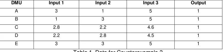
Counterexample 3. Let us assume that we have observed five DMUs that produce one output from the consumption of three inputs (see Table 1). Considering
100,000
M , and the evaluation of the performance of unit E, we obtain, applying (12), that
1
, 2 3
E E
C x y ,
2
, 2 3
E E
C x y and
3
, 0.43
E E
C x y . In this way, we
conclude that C x y
E, E
0.43 . However, unit C produces the same quantity of output and dominates unit E in the sense of Pareto. If we use the inputs of unit C for evaluating unit E, we get 2.81 3
, 2.22 3
and 4.63 5
. This leads to the followingsum of input contractions:
3
1
1 i 0.41 0.43
i
17
contraction to the strongly efficient frontier does not always coincide with the smallest
0, 0
kC x y , k 1,...,m.
<Insert Table 1 approximately here>
In summary, as we are aware, none of the existing approaches allows the determination of the closest Pareto-efficient targets in the oriented framework to be dealt with in a suitable way. In the next section, we will propose a solution to this problem. In particular, we will introduce a new methodology based on Bilevel Linear Programming.
3. A solution based on Bilevel Linear Programming
In this section, we first briefly review the mainly notions related to Bilevel Programming in order to introduce, in the second part of the section, an approach on these grounds to determine the closest targets and the least distance through oriented models in DEA.
A Bilevel Programming model refers to a mathematical programming problem where one of the constraints is an optimization problem. This theory has been successfully applied to model different real situations with a common feature: the existence of a hierarchical structure (see Wu, 2010). A Bilevel Programming problem where both the objective functions and the constraints are linear is called a Bilevel Linear Programming problem. Denote by z Z Rp and t T Rq the decision variables corresponding to the first and second level, respectively. The general formulation of a Bilevel Linear Programming (BLP) problem is as follows:
1 1
,
1 1 1
2 2
2 2 2
. .
,
. .
,
0,
0
z t
t
Min c z d t
s t
A z B t
b
Min c z d t
s t
A z B t
b
z
t
(13)
18
Regarding the solutions of a BLP problem,
z t*, *
0 is a feasible solution of (13) if t* is an optimal solution of the lower level program with zz* and, at the same time,A z
1 *
B t
1 *
b
1 . In this way,
* *
,
z t is an optimal solution if additionally
* *
1 1 1 1
c z
d t
c z d t
for all feasible solution
z t, of (13), beingc z
1 *
d t
1* the corresponding optimal value of the BLP problem.Now we are ready to introduce the model that permits the closest Pareto-efficient targets in the output-oriented case to be determined. The input-oriented case could be derived by analogy. The key idea is to exploit the hierarchical structure of the BLP problems, using the measure that needs to be determined as the higher level problem and the lower level problem being the output-oriented weighted additive model that, by Lemma 1, is able to characterize the belonging to the strongly efficient frontier in the oriented case by its optimal value. Let us assume that we are interested in determining the Russell output measure under the least distance criterion. In this case, the model to be solved is the following:
1 0 0 1 1 0 0 1 (14.1) . .
, 1,..., (14.2)
, 1,..., (14.3)
1, (14.4)
0, (14.5)
(14.6) . .
, 1,..., (14.7)
VRS VRS VRS VRS VRS s r r
j ij i j E
j rj r r j E j j E s r r r s r r r
j ij i j E
j rj r r j E
Min s s t
x x i m
y y r s
w s
Max w s
s t
x x i m
y y
, 1,..., (14.8)1, (14.9)
1, , , 0, , (14.10)
VRS
r
j j E
r j r j
s r s
s r j
19
In (14) the higher level problem coincides with the Russell output measure except for the fact that the objective function is minimized instead of maximized as happens with the traditional definition of the Russell output measure (Färe et al., 1985, p. 149), while the lower level problem matches (8) when the evaluated output vector is
1 10y ,...,
sys0
.The next proposition states that the optimal value of (14) equals the Russell output measure under the philosophy of seeking the least distance to the strongly efficient frontier of the production possibility set.
Proposition 2. Let
*, *,s*,
*
be an optimal solution of (14). Then,
*
1 10 0 0 0
1 1
1
1
:
,...,
;
s s
r r s s VRS
r r
Min
y
y
D y P
x
s
s
.Proof. See Appendix.
Regarding the weights
w
r in (14), we will assume from now on thatw
r
1
, As for the implementation of the BLP problem, even in the case of all functions being linear in (14), the problem is not trivial from a computational point of view (Shi et al., 2006). Solution techniques for BLP may be classified into two major groups. A possibility is to transform the original problem into a single optimization problem by applying the well-known Karush-Kuhn-Tucker (KKT) optimality conditions of the lower level problem. The other group uses enumeration techniques. In this paper, we will particularly use the KKT optimality conditions in order to solve (14). Accordingly, (14.6)-(14.9) must be substituted by (15.1)-(15.9).1,..., .
20
0
0
1 1
, 1,..., (15.1)
, 1,..., (15.2)
1, (15.3)
0, (15.4)
0, 1,..., (15.5)
1, 1,..., (15.6)
0, (15.7)
VRS
VRS
VRS
j ij i i j E
j rj r r r j E
j j E
m s
i ij r rj j j VRS
i r
i i r
j j VRS
i
x l x i m
y y s r s
x y j E
e i m
r s
j E
l e
0, 1,..., (15.8)
, , , , 0, , (15.9)
i
i i r j i
i m
l
e i j
(15)
Constraints (15.7)-(15.8) are not linear. Nevertheless, restrictions of this nature are not difficult to be implemented by means of a Special Ordered Set (SOS)4 (Beale and Tomlin, 1970).
4. Empirical illustration: Efficiency of schools using PISA data
This section includes an empirical illustration with real data applying the methodology proposed in this paper. In particular, we use Spanish data from the PISA (Programme for International Student Assessment) 2012 survey, where data from student and school questionnaires (with students and school level information, respectively) were merged. This dataset provides results on the performance of 15 year-old students in different competences as well as other factors potentially related to those results such as variables representing student background, school environment or educational provision.
Following the well-established literature on school efficiency (e.g. Agasisti and Zoido, 2015; De Witte and Lopez-Torres, 2015; Santin and Sicilia, 2015; Crespo-Cebada et al., 2014), we select the results from a standardized test as educational outputs and three usual inputs in education production functions such as the students (raw material), infrastructures (school resources) and teachers (human capital). Table 2 reports the descriptive statistics for these five variables considering the total number of
4
21
schools (902) included in the sample. A detailed explanation of the specific indicators considered in the empirical analysis is provided below.
- As a proxy for the quality of students in the school, we use the average of the socio-economic status of students in the school, represented by the ESCS index, which provides a measure of family background that includes the highest levels of parents´ occupation, educational resources and cultural possessions at home. Since the original values of this variable presented positive and negative values, all of them were rescaled to show positive values.
- As a proxy for the availability of material resources, we use an index created by PISA analysts (SCMATEDU) from the responses given by school principals regarding several educational resources such as computers, educational software, calculators, books, audio visual resources or laboratory equipment. In this case, we have also rescaled the original values to assure that all values are positive.
- The inverse of the student-teacher ratio, i.e., the number of teachers per (hundred) students (TEACHERS), as a proxy for human resources employed by schools.
- The output variables are represented by the averaged test scores achieved by students belonging to the same school in reading and maths. Regarding this point, it is worth noting that PISA reports five plausible values randomly drawn from the estimated distribution of results for each student according to their answers to the questions in the test (see OECD, 2012 for details). Those plausible values can be interpreted as a measure of their performance in order to approximate the real distribution of the latent variable being measured (cognitive skills) (Mislevy et al., 1992; Wu, 2005).
<Insert Table 2 approximately here>
Table 3 shows a summary of the results obtained with the approach proposed in this paper, model (14). The mean of the technical efficiency of the Spanish sample is 1.122 (1.135 in reading and 1.109 in maths), which means that, on average, the schools could increase their outputs levels by 12%, needing a greater effort in the reading dimension, without changing their resources. With regard to the resolution of the 902 optimization programs, we used CPLEX to solve the different problems and code in C on a CPU AMD Phenom II X6 1075T (hexa-core) with 3 GHz and 16 RAM GB. In this respect, the average time of execution was 10.782 seconds, i.e., a total amount of around 3 hours.
22
5. Conclusions
In this paper, we have shown that all the existing approaches to determine the closest Pareto-efficient targets in DEA present some weaknesses when they are applied or adapted to the oriented framework, when the interest of the firm/organization is to expand its output bundle without requiring any increase in its inputs or to contract its input bundle without requiring a reduction in its outputs.
To deal with this problem in a suitable way, a new methodology based upon Bilevel Linear Programming was introduced to determine the desired targets in the case of using a new version of the Russell oriented measure. Its implementation is grounded on the application of the Karush-Kuhn-Tucker (KKT) optimality conditions to the lower level problem and Special Ordered Sets (SOS).
Finally, the new approach was illustrated through an empirical analysis using data on the 902 Spanish schools participating in PISA 2012. The results show that there is room for improvement, especially in reading (one of the outputs selected). Likewise, the computation time is relatively low considering the size of the available sample.
Acknowledgements
23
References
Agasisti, T. and Zoido, P. (2015). The Efficiency of Secondary Schools in an International Perspective: Preliminary Results from PISA 2012 (No. 117). OECD Publishing.
Amirteimoori, A. and Kordrostami, S. (2010). A Euclidean distance-based measure of efficiency in data envelopment analysis. Optimization 59: 985–996.
Ando, K., Kai, A., Maeda, Y. and Sekitani, K. (2012). Least distance based inefficiency measures on the Pareto-efficient frontier in DEA. Journal of the Operations Research Society of Japan 55: 73–91.
Aparicio, J., Ruiz, J.L. and Sirvent, I. (2007). Closest targets and minimum distance to the Pareto-efficient frontier in DEA. Journal of Productivity Analysis 28: 209–218. Aparicio, J. and Pastor, J.T. (2013). A well-defined efficiency measure for dealing with
closest targets in DEA. Applied Mathematics and Computation 219: 9142–9154. Aparicio, J. and Pastor, J.T. (2014a). On how to properly calculate the Euclidean
distance-based measure in DEA. Optimization 63(3): 421–432.
Aparicio, J. and Pastor, J.T. (2014b). Closest targets and strong monotonicity on the strongly efficient frontier in DEA. Omega 44: 51–57.
Baek, C. and Lee, J. (2009). The relevance of DEA benchmarking information and the least-distance measure. Mathematical and Computer Modelling 49: 265–275. Banker, R.D., Charnes, A. and Cooper, W.W. (1984), Some Models for Estimating
Technical and Scale Inefficiencies in Data Envelopment Analysis, Management Science 30: 1078–1092.
Beale, E.M.L. and Tomlin, J.A. (1970). Special facilities in a general mathematical programming system for non-convex problems using ordered sets of variables. In Proceedings of the Fifth International Conference on Operational Research, edited by Lawrence, J., pp 447-454. London: Tavistock Publications.
Briec, W. (1997) Minimum distance to the complement of a convex set: duality result. Journal of Optimization Theory and Applications 93: 301–319.
Briec, W. (1998). Hölder distance function and measurement of technical efficiency. Journal of Productivity Analysis 11: 111–131.
24
Briec, W. and Lesourd, J.B. (1999) Metric distance function and profit: some duality results, Journal of Optimization Theory and Applications 101(1): 15-33.
Briec, W. and Leleu, H. (2003). Dual representations of non-parametric technologies and measurement of technical efficiency. Journal of Productivity Analysis 20: 71– 96.
Chambers, R.G. and Mitchell, T. (2001) Homotheticity and Non-Radial Changes. Journal of Productivity Analysis 15: 31–19.
Charnes, A., Cooper, W.W. and Thrall, R.M. (1991) A structure for classifying and characterizing efficiency and inefficiency in data envelopment analysis. Journal of Productivity Analysis 2: 197–237.
Cherchye, L. and Van Puyenbroeck, T. (2001). A comment on multi-stage DEA methodology. Operations Research Letters 28: 93–98.
Coelli, T. (1998) A multi-stage methodology for the solution of orientated DEA models. Operations Research Letters 23: 143–149.
Cooper, W.W., Park, K.S. and Pastor, J.T. (1999) RAM: A Range Adjusted Measure of Inefficiency for Use with Additive Models, and Relations to Others Models and Measures in DEA, Journal of Productivity Analysis 11: 5-42.
Cooper, W.W., Seiford, L.M. and Tone, K. (2007) Data envelopment analysis: a comprehensive text with models, applications, references and DEA-solver software. Springer.
Crespo-Cebada, E., Pedraja-Chaparro, F. and Santín, D. (2014). Does school ownership matter? An unbiased efficiency comparison for regions of Spain. Journal of Productivity Analysis, 41(1), 153-172.
De Witte, K. and López-Torres, L. (2015). Efficiency in education. A review of literature and a way forward, Journal of Operational Research Society, forthcoming.
Färe, R., Grosskopf, S. and Lovell, C.A.K. (1985) The Measurement of Efficiency of Production, Kluwer Nijhof Publishing.
Frei, F.X. and Harker, P.T. (1999). Projections onto efficient frontiers: theoretical and computational extensions to DEA. Journal of Productivity Analysis 11: 275–300. Fukuyama, H., Maeda, Y., Sekitani, K. and Shi, J. (2014a). Input-output substitutability
25
Fukuyama, H., Masaki, H., Sekitani, K. and Shi, J. (2014b). Distance optimization approach to ratio-form efficiency measures in data envelopment analysis. Journal of Productivity Analysis 42: 175-186.
Fukuyama, H., Hougaard, J.L., Sekitani, K. and Shi, J. (2016). Efficiency measurement with a nonconvex free disposal hull technology. Journal of the Operational Research Society, 67: 9–19.
Gonzalez, E. and Alvarez, A. (2001). From efficiency measurement to efficiency improvement: the choice of a relevant benchmark. European Journal of Operational Research 133: 512–520.
Grifell-Tatje, E., Lovell, C.A.K. and Pastor, J.T. (1998) A Quasi-Malmquist Productivity Index. Journal of Productivity Analysis 10: 7–20.
Koopmans, T.C. (1951) Analysis of Production as an Efficient Combination of Activities, in T.C. Koopmans (Ed.), Activity Analysis of Production and Allocation, New York, John Wiley.
Lovell, C.A.K. and Pastor, J.T. (1995) Units Invariant and Translation Invariant DEA Models. Operations Research Letters 18: 147–151.
Lozano, S. and Villa, G. (2005). Determining a sequence of targets in DEA. Journal of Operational Research Society 56: 1439–1447.
Mislevy, R.J., Beaton, A.E., Kaplan, B. and Sheehan, K.M. (1992). Estimating population characteristics from sparse matrix samples of item responses. Journal of Educational Measurement 29(2): 133–161.
OECD (2012), PISA 2009 Technical Report, PISA, OECD Publishing, Paris.
Pastor, J.T., Ruiz, J.L. and Sirvent, I. (1999) An Enhanced DEA Russell Graph Efficiency Measure, European Journal of Operational Research 115: 596–607. Pastor, J.T. and Aparicio, J. (2010) The relevance of DEA benchmarking information
and the Least-Distance Measure: Comment. Mathematical and Computer Modelling 52: 397–399.
Portela, M.C.A.S., Castro, P. and Thanassoulis, E. (2003). Finding closest targets in non-oriented DEA models: The case of convex and non-convex technologies. Journal of Productivity Analysis 19: 251–269.
26
Ruiz, J. L and Sirvent, I. (2010) A DEA approach to derive individual lower and upper bounds for the technical and allocative components of the overall profit efficiency. Journal of the Operational Research Society 62: 1907–1916.
Ruiz, J.L. and Sirvent, I. (2015) Common benchmarking and ranking of units with DEA. Omega (in press).
Ruiz, J.L., Segura, J.V. and Sirvent, I. (2015) Benchmarking and target setting with expert preferences: An application to the evaluation of educational performance of Spanish universities. European Journal of Operational Research 242: 594– 605.
Santín, D. and Sicilia, G. (2015). Measuring the efficiency of public schools in Uruguay: main drivers and policy implications. Latin American Economic Review, 24(1), 1-28.
Shi, C., Zhang, G., Lu, J. and Zhou, H. (2006) An extended branch and bound algorithm for linear bilevel programming. Applied Mathematics and Computation 180: 529–537.
Tone, K. (2001) A slacks-based measure of efficiency in data envelopment analysis, European Journal of Operational Research 130: 498–509.
Wu, D.D. (2010) Bilevel programming Data Envelopment Analysis with constrained resource, European Journal of Operational Research 207: 856–864.
Wu, M. (2005). The role of plausible values in large-scale surveys. Studies in Educational Evaluation 31(2): 114–128.
27
Appendix
Proof of Lemma 3: Let us assume that *0 0
CRS j j j E
x
x
. Let us define
* *
0 0
.
CRS j j j E
x
x
In this way, by (1),
x y0*, 0*
TCRS . Moreover, note that
j
E
CRS such that
*j0 0, since otherwise constraint (8.2) would be violated for 0s
y
R
[really it is sufficient if 0 s \ 0
s
y R ]. Consequently,
x
0*
0
. By the definition ofx
0*,* 0
0 0 *
0
1
x
x x
x
. This implies that, under CRS, 0*
0* 0*
0 *0 0*0 0
,
,
CRSx
x
x y
x
y
T
x
x
.Therefore, 0 *
0 0
* 0
CRS
x
y P x
x . However,
* * 0 0 0 * 0 r r x y y
x , r 1,...,s , since
* 0
s
y
R
and
y
0
R
s . Thus, y0* s
PCRS
x0
, which is a contradiction to Lemma 2. So, by(8.1), *0 0
CRS j j j E
x
x
. ■Proof of Proposition 1: (i) Let
,s v u d b, , , ,
be a vector that satisfies constraints 11.2-11.12. From this solution, it is possible to generate yDˆ
y P0; CRS
x0
asCRS r j rj
j E
y
y
, r 1,...,s . Let us note that, by (1),
x y,
TCRS , with0
:
CRS j j j E
x
x
x
, and, consequently, yPCRS
x PCRS