Munich Personal RePEc Archive
Impact of Oil Price and Its Volatility on
Stock Market Index in Pakistan:
Bivariate EGARCH Model
Naurin, Abida and Qayyum, Abdul
Pakistan Institute of Development Economics, Islamabad, Pakistan,
Pakistan Institute of Development Economics, Islamabad, Pakistan
April 2016
Online at
https://mpra.ub.uni-muenchen.de/70636/
Impact of Oil Price and Its Volatility on Stock Market Index
in Pakistan: Bivariate EGARCH Model
By
Abida Naurin1 and Abdul Qayyum2
ABSTRACT
Oil is becoming as an important determinant which affects the macroeconomic activities and the stock market indices in unusual patterns among various parts of the globe particularly since the first oil crisis in 1973. Also Petroleum products are recognized to be the essential source of energy and power throughout the world and gaining substantial importance as a tool for endurance and security of developed nations. The research study targets to explore the impact of oil price and its volatility on Stock market index in Pakistan from the period 1991:M11 to 2014:M12. In this study we used the financial time series econometrics techniques; first applied the Box-Cox transformation on the data which suggested log transformation is required for all series. As data used will be monthly, Beaulieu and Miron (1992) seasonal unit root test is used if stationarity is present in the data. All variables hold unit root at zero frequency and become stationary at first difference. Further to confirm if co-integration relationship exists between the variables we have estimated Engle and Granger (1987) two-step method. And finally Bivariate EGARCH model is applied to scrutinize the impact of oil price volatility Stock market index. Bollerslev and Wooldridge (1992) proposed this model which is projected by using Maximum likelihood method. Hence the findings of Bivariate EGARCH model suggested the direct association between oil prices and Stock market Index. It means SPI is positively affected by oil
prices. In case of Pakistan, asymmetric impact is positive but statistically insignificant at α=.05
(Level of significance). But in case of oil price volatility Bivariate EGARCH model, it is negative and statistically insignificant. The summation of Beta Coefficients of ARCH and GARCH suggests that the volatility shocks in the SPI have been highly continual and became extinct rather slowly in case of Pakistan.
Keywords: Oil prices, Volatility of oil prices, SPI, Box Cox Transformation, Beaulieu and
Miron, Co-integration, Bivariate EGARCH, Pakistan.
1
Abida Naurin, an MPhil Scholar at the Department of Econometrics and Statistics, PIDE and
2
1.
Introduction
Oil prices has captured the attention of new investigators as a significant factor which
have an effect on macroeconomic actions and the stock market indices in different ways over the
globe particularly since 1973 when the first oil crisis occurred. Oil is measured as a most integral
source of energy in the world and achieving substantial significance as a mean of urbanized
countries’ protection and continuous existence. According to Hamilton (1983), remarkable
increase in the prices of crude oil resulted in the seven out of eight postwar downturns in the
United States. Such conclusions and estimations have provided the base for the researchers to
study oil as a significant determinant while assessing the economic activities in any country. Oil
is the biggest need of every country that’s why the alterations in oil prices affect the financial
environment of industrial and developing states.
Consequently, stock market becomes less attractive due to higher interest rate that has to
increase by policy makers due to pressure. The value of stocks declines due to the anticipation
that interest rate to be higher and increase in oil costs decrease the cash flows of companies so
the threat to stock market is the oil price flourishing. So, oil price change besides affecting
production and utilization like other merchandise can also be source of change in behavior of
depositors and stock prices.
Production cost includes oil as a major element.The development of a financial system is
greatly dependent upon the rate of investment in the country. The function of stock market is to
make available a platform which channelizes funds from excess to lacking units for fruitful
investment. The movement in stock market causes the fluctuation in demand and supply of the
underlying assets which represent the equity holding of the company by the investors. The price
of stock denotes the present value of the potential cash flow streams of the company. In this
context the presence of optimism in the market would lead to rise in stock prices, while on the
other side the pessimistic thoughts would cause the decline in the stock index. Hence, the
mentioned is the reason that the stock market can be considered as the index of the economy.
Stock exchange is very important because it participate very animated role for the advancement
of the financial sector for all the countries Siddiqui, (2014).
Pakistan has three major stock exchanges including (KSE) Karachi Stock Exchange,
(ISEI) Islamabad Stock Exchange and (LSE) Lahore Stock Exchange. Karachi Stock Exchange
.Because it plays vital role for the development of the country. Stock markets offer the platform
where all investor are fully contributing not only local investor. Therefore, foreigner investors
are investing the new business came to exist now it is positive sign for the development in the
country.
The developed as well as developing economies are facing the problem of oil prices
unpredictability. Linear model is used by the majority of the offered studies on this field. By
relaying on the market arrangement or asymmetric market information this model ignores the
nonlinear factors. Econometric analyses like co-integration and Granger causality test are applied
to examine this issue. These techniques are not appropriate for proper results. Our study is
important because, most of the relationship in the financial markets is non-linear in its behavior.
The data frequency is low, thus using monthly data will give more consistent and efficient
results. Hamilton (1983) was first who studied this relationship, while Jones and Kaul (1996)
studied this effect on stock market. But still there is very little research to analyses the
relationship and forecast it. A lot of researches are made for data of UK or USA or EU or
developed or industrial countries while the studied on BRIC and GCC countries are also found.
But only one or two paper discusses the relationship in Asian stock markets and that is also in
panel data. This study is being conducted with the key purpose to cover this space in literature by
using better technique of estimation of non-linear model. Increase and decrease in the oil prices
do not have similar affect. Park and Ratti (2007) demonstrate in their study that decline in oil
price has less influence on the economy than increase in its price. I have decided to explore the
asymmetric effects of oil price changing on KSE-100 Index in Pakistan because of its practical
importance. So there is a gap in literature that impact of oil price volatility on stock market index
in Pakistan has not been studied and observed for said relationship.
The main objective of this study is to investigate the impact of oil price and its volatility
on Stock market (KSE-100 Index) in Pakistan from the period 1991:M11 to 2014:M12. The
other objective of the study is to examine the long run impact of oil price and its volatility on
SPI. We also found the asymmetric effects of oil price in case of Pakistan.
This study is arranged as follows; section 2 demonstrates the salient features of Oil sector and
Stock market in Pakistan. Section 3 describes literature review of previous studies at national and
international level, followed by Econometric Methodology in section 4, results and discussion is
2. Salient Features of Oil Sector and Stock Market in Pakistan
Geopolitical issues, OPEC and non OPEC supply commotion are the main reason behind
the fluctuations in prices of oil. Initially the prices of oil were organized by US before the 1971
then this control was shifted to OPEC after a decade of its formation. OPEC had five members in
1960 after its formation but it has turned to six in1971.The world oil price was set $3.5/ barrel in
1972. The price of oil tripled in1974 in international market because many Arab oil exporting
countries including Iran impediment on western countries and United States and shortened its
production. This was happened when Egypt and Syria attacked Israel in1973 and United States
and other western countries started supporting Israel. But afterward these price are remained
smooth in between 1974-78.
However after Iranian revolution the supply of oil again disturbed and in response prices
increased again in 1979 but soon they have controlled their production. In 1980 Iraq assaulted
Iran and price went up because of distraction in the production of both countries. However due to
production of non OPEC and geopolitical stability price got stable in 1980’s. Commonly it is
experienced that oil prices in its market place went down yet in case of Saudi its income went
upward due to oil extraction and domestic low price. In December 1986 OPEC had fixed an oil
price at 18 $/container but that price was not prevailed for longer and soon decreased in the start
of 1987. Due to supply shortage in 1990 Iraq-Kuwait war played an essential role to increased oil
prices. After this war the oil price slow down noticeably till 1994 and meet the prices that was
prevailed in 1973.
When Iraq attacked Kuwait price merely increased for short but for the rest of decade of
1990’s it remained stable. In late 1990 the oil production was cut by OPEC due to supply
shortage the prices of oil was greater than before in developed and developing nations. Later on
the prices remain stable as the non OPEC countries increased their production especially Russia.
Afterward prices are revived in 1998 because of supply shortage of oil OPEC and sustained it at
the level of 1.72 million containers in April, 1999. Previously OPEC has try to allocate oil
supply quota among its members in 1982-85 but it was failed to experienced due to opposition of
its members particularly Saudi Arabia that shorten its supply as oil prices were too low. Again in
mid-1986 a try was made to associate the oil prices with its oil market to stable prices at less the
The oil war remain continue and US invaded Iraq in 2003 and prices of oil started
increasing due to the growing demand for oil in developed and emerging economies and also
production disturbance in Iraq and Venezuela. This price scrambling was demand driven and
price reached at 97 US $ in 2008. When the oil demand increased in Asian countries in 2009
OPEC again decreased its supply that leads to shortage of 400,000 barrel/ day due to civil war in
Libya. Because of this growing trend in demand in developing and developed nation the price of
oil continued to increase afterward 2010 and never stops.
These shocks about oil prices depict that it have great impact on Stock Price Index of oil
importing country (Pakistan) either directly and indirectly. With collaboration these external
shocks Pakistan oil prices are also affected by the internal shocks due to various natural disasters
and political conflicts prevailing within country. The earth quake of 2005 in northern areas of
Pakistan badly affect its economy. Yet before that GDP was high and stable in 2004. Another
natural disaster was and political conflicts prevailing within country. Another natural disaster
was 2011 flood that ruins agriculture and infrastructure badly and tumbled down the economy as
a whole. Such miscue leads to high import prices and create shortage of recourses due to high oil
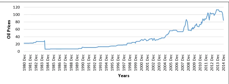
prices that is the one of the major input in almost all sectors economy. The oil prices trend is
[image:6.612.73.542.442.614.2]shown in figure 2.1.
Figure 2.1: Current Oil Prices in Pakistan (1980-2014)
Source: Monthly Statistical Bulletins of Pakistan.
3. REVIEW OF LITERATURE
There are many studies on the subject of energy price, especially in case of oil prices and
Masih et al (2011), analyzed oil price volatility and stock market rise and fall in a rising
market: Evidence from South Korea. To examine the stochastic properties and long run
dynamics between the macro-economy, the stock markets, the instruments of monetary policy
and the oil price fluctuations are the aims of this study. For this purpose, secondary data is used
from May 1988 to Jan2005. By using the VECM model the examiners look into the impact of oil
price changes and volatility on real stock returns, industrial production and interest rate. For
further analysis, modern time series techniques in a co-integrating framework, Variance
Decomposition and Impulse response function have also been employed. This study exposed that
oil price movements significantly affect the stock market and the main channel of short run
adjustment to long run equilibrium are real stock returns.
Bodenstein et al (2012), examined the how monetary policy makers should respond to oil
price fluctuations and conclude that the best central bank policy response to oil price fluctuations
depends on why the price of rudimentary oil has changed. For this purpose, multi-country DSGE
model has been employed that is estimated by the method of maximum likelihood based on data
for 1984-I through 2008-III quarterly. The major findings of this study are to explain that no two
structural shocks justify the same monetary policy response and optimal monetary policy is well
approximated by a policy rule that targets the output gap and attaches zero weight inflation.
Further, find that oil trade greatly enhances the welfare gains from international monetary policy
coordination.
Dhaoui and Kharief (2014) examined the practical relationship between oil price and
stock market returns and unpredictability: confirmation from international developed markets for
the period from January 1991 to September 2013 for eight developed countries. An EGARCH-M
model has been used as an econometric method. The study concluded that oil price and stock
market returns are strongly negatively connected in seven of the selected countries. Oil price
changes have no significant effect on the stock market of Singapore. On the instability of returns,
oil price changes have significant for six markets and no much effect on the others.
Le and Chang (2011) studied on “The impact of oil price fluctuations on stock markets in
developed and emerging economies. The aim of this study was to examine the response of stock
markets to oil price volatilities in Japan. Singapore, Korea and Malaysia by applying the
1986:01- 2011:02. The results show that response of stock market to oil price shocks diverge
considerably across markets. The stock market showed negative response in Malaysia while
positive in Japan but the signal in Korea and Singapore was blurred. Further the stock market
ineffectiveness was find out, among others, seemed to have the slow reactions of the stock
market to aggregate shocks such as oil price surges.
Sandusky’s (1999) study on the US economy also shows that oil price volatility shocks
have asymmetric effects on the economy. By evaluating the desire response functions, he shows
that movements in stock returns can be explained by movements in oil prices: after 1986,
furthermore, larger portion of forecast error variance in real stock returns is explicated by the oil
price movements than the interest rates. The results finally recommend that positive shocks to oil
prices slow down real stock returns while shocks to real stock returns have positive impacts on
interest rates and industrial production.
Jones and Kaul (1996) however report that the reaction of the United States and Canadian
stock markets to oil price shocks can be completely enlighten on the basis of changes in the
expected value of future real cash flows. This evidence is valid but is weaker for the UK and
Japan.
Siddique (2014) conducted a study on “Oil price fluctuation and stock market
performance-The case of Pakistan”. The goal of this study is to investigate the impact of oil price
fluctuation on the stock market performance in Pakistan and KSE-100 index has been considered
for analysis as an accurate representative sample of the country’s stock markets. The annual time
series data has been used from 2003 to 2012 for analysis. In this study , first of all find the
descriptive statistics of all the variables after that find the correlation matrix and then estimate
the simply regression. This study concludes that an optimistic and statistically significant
relationship exists between oil price and other explanatory variables and stock market
performance in Pakistan.
Ansar and Asghar (2013) examined the impact of oil prices on the CPI and stock market
(KSE-100 index). For this reason the pollsters by using the secondary data employed the multi
regression method from January2007 to August2012. The study revealed that there is positive
but not much stronger relationship among the oil prices, CPI and KSE-100 index. Jawad (2013)
study is to explore the impact of oil price volatility on the economic growth of Pakistan. For this
the researcher estimated the linear regression by using the secondary data from 1973 to 2011.To
check the stationary, unit root test i-e Augmented Dickey-Fuller Test has been employed. This
study revealed that oil price volatility has immaterial impact on Gross Domestic Production.
Fatima and Bashir (2014) studied Oil price and stock market fluctuations: Emerging
Markets( A comparative study of Pakistan and China) The foremost objective of this study has to
look at the volatility of international oil prices and stock market of emerging markets of Asia so
the evidence was taken from China and Pakistan. The data is used 1st January 1998 to 31st
December 2013. The monthly data is used for Stock market, Brent oil prices, exchange rate and
CPI of respective countries. Multivariate Co-integration Analysis has done along with Vector
Error Correction Model. Firstly, OLS regression has been applied and then unit root test to check
the stationarity of data. The results discovered that all the variables have integrated at first
difference i.e. I(1). When variables became stationary a differencing then co-integration analysis,
Granger causality test and VECM model applied for further analysis. The results revealed that oil
prices negatively affected the stock markets in emerging markets such as these countries are oil
importing countries. To end Impulse Response and Variance Decomposition that forecast the
impact of oil on stock markets. Then asymmetric effects have been observed in the stock
markets.
The above literatures have employed different methodologies to fulfill their different
objectives. Some used panel data and some used time series data. Majority of the studies reveal
that oil prices has positive impact on stock market. If we examine the literature review in
context of Pakistan There are number of issue in the above studies, as there are used small data
sets for the time series which can’t fulfill the basic criteria of minimum data/observation
selection of time series analysis e.g. Siddique (2014), Ansar and Asghar (2013) and Jawad
(2013). Particularly financial data is skewed and leptokurtic in their behavior, which violate the
assumption of normality. When data set is not normal and shows volatility in it then linear
models are not suitable. For this, use volatility modeling; volatility of a series is generally
measured by its conditional variance. Due to volatility clustering there is ARCH effect in the
series because series is conditionally depends on its lags. To capture this effect didn’t use the
monthly time series data while Beaulieu and Miron unit root test is appropriate for monthly time
series. In the methodology, auto correlation exists so the suggested results are biased. So, there
exists a gap in the literature. To solve all these problem mention above can be solve under the
structure of non- linear models i.e. ARCH family, with the help of large data set.
4. METHODOLOGY
Nelson (1991) has developed the Exponential Generalized Autoregressive Conditional
Heteroskedasticity (EGARCH) model. Braun, et al. (1995), Kroner and Ng (1996, 1998), Henry
and Sherma (1999) and Engle and Cho (1999) have extended Exponential Generalized
Autoregressive Conditional Heteroskedasticity (EGARCH) model in bivariate version. Nelson
(1991) argues that market information affects the conditional variances and this affection varies
from information to information and to capture asymmetric adjustment margins effect he set up
an EGARCH model. Engle and Ng (1993) recommends a standard measure to how news
information can be incorporated in to the volatility estimates. In order to better estimation and
scantest news information impact curves to the data, a number of new candidates for modeling
time fluctuating volatility are introduced and compared. These models permit numerous types of
asymmetry in the effect of news information on volatility. Yoo (1987) and lee (1994) say that the
error-correction term is a critical component to describe the conditional mean of the
co-integration variables. EC-GARCH model contain the error-correction term in the GARCH model
which proposed by Lee (1994). Empirical results in Enders and Granger (1998) conclude that the
asymmetric ECM could describe the long run equilibrium relation.
In this paper, we use the model extended with error correction term in the mean equation
to establish the Bivariate EGARCH model. Further Engle and Granger (1987) two step method is
used for the presence of cointegrating relationship between the variables. As a first step we
estimated the long run equation and then apply unit root test on the residual from the
cointegrating equation.
The Engle-Granger two step method for stock price index is
……… (4.1a)
Where log of Stock price index is, is log of oil price, is residual from
cointegrating equation and is residual from the equation of unit root test which is supposed to
be white noise.
The Bivariate EGARCH (p, q) model for the stock market consists of two equations such
as:
∑ ∑ … … (4.2a)
( ) (| | (| |))
+ (| | (| |)) ……… … … … (4.2b)
Where; i = 1, 2….p and j = 0, 1….q tΩt-1 ~ N [0, (spit) ²]
The variables used in the above equations are as follows:
= Returns on Stock Market
( )= Variance of stock market returns
= Log difference of oil prices
= Variance of log of oil prices
= Error correction term
= Random variable
The equation (4.2a) is conditional mean equation of returns on stock market ( ).
That is dynamic error correction model. The random variable (i.e., εt) is supposed to have zero
mean and conditional variance. Later the second equation of the model (i.e., 4.2b) indicates the
conditional variance of the stock market returns. This equation depends upon the lagged value of
innovation of log SPI and the log of oil prices, lag of conditional variance of the stock market
returns and the terms to detect asymmetric effect. The parameter shows last period forecast
variance and indicates news impact of stock market returns. While the parameters and
shows the last period forecast variance and the asymmetric impact of oil price respectively in the
conditional variance of stock market returns. Additional, the θ’s permit asymmetry news impact
from SPI. The estimated parameter of GARCH term that is shows persistence of volatility.
Data for this study is taken from the period of 1991-11 to 2014-12. The variables in this
regard used are current oil prices and KSE-100 Index of Pakistan. Oil prices (OP)-oil
Pakistan. The sample period of KSE-100 Index taken from State Bank of Pakistan (SBP). Here is
the description of econometric techniques that we will use in this study for our findings.
It is important to test the time series before building a model, if there is a need to
transform the data. As transformation ensure proper functional form of the model. Before the
estimation of univariate and multivariate models, it is necessary to transform the dependent and
independent variables. Power family of transformation is modified by “Box and Cox” in
1964.Further modify the box-cox transformation by using the Geometric mean in the
transformation. So we applied Box-Cox transformation in this study by using following formula:
( ) ( ) If ………. (4.3)
( ) = if ……….. (4.4) L (λ) = - T/2(1+LN2π + LN RSS/T) ………... (4.5)
The maximum L (λ) value of λ will suggest the type of transformation of the series. Before
estimation of Bivariate EGARCH model we have to check the stationary of the series. The test
was developed by Beaulieu and Miron (1993) to test the seasonal and non-seasonal unit root (i.e.
unit root at zero, biannual and annual frequency) in monthly time series. It extended to the
Frances (1991) U.R Test by generating 12 series to detect the complex U.R separately. Beaulieu
and Miron proposed the test of unit root in monthly data. The null hypothesis are
H0: 1 2...12 0
H1: At least one of them is not zero
To test the unit root in monthly series Beaulieu and Miron suggest estimation of the following equation.
∑ ∑ … (4.6)
The variables can be generated by following equations. Where
We have estimated the equation with OLS. And test for the serial autocorrelation of the
residuals. For this we have used LM test at 1st and 12th lag. If the residuals are not white noise
then we added lags of dependent variable until the error terms of the series is whiten. Hypothesis
which is tested for this test varies between even and odd. First two coefficients .i.e. and are
tested individually using t-test and remaining are tested using F-test by applying the Wald Test.
The zero frequency unit root ( = 0) and bi-annual frequency unit root ( = 0) are
tested using left sided t-statistics.
While the complex roots are tested by using joint test (F-test). If all = 0, then we apply (1 ) filter.
If 0 data are stationary and use seasonal dummies.
In this study Engle and Granger Two- Step Method is used for cointegration. Engle and
Granger (1987) offered the two step co-integration test also called as residual based test. But this
test is not appropriate for more than two variables. This method is following as:
Step 1
While moving with the step 1 of Engle and Granger (1987) approach with regression of
the variables, it is necessary to include variables expected to be co-integrated and have sustained
shocks on the equilibrium. The variables that have sustained the shocks are termed as exogenous
shocks and basically are included in the form of dummy variable. As a first step we will be
estimated the long run equation and then apply unit root test on the residual from the
co-integrating equation.
The Engle-Granger two-step method for price Stock price index can be performed as:
𝑡 = + 𝑋𝑡 + 𝑡 ……… (4.7)
Δ = ρ + Δ + Δ + … + Δ + … ………... (4.8)
∴ ~ N (0, )
Where = (L ) is log of stock price index respectively, 𝑋= (L ) is log of oil
price. is residual from co-integrating equation and is residual from the equation of unit root
test which is assumed to be white noise. After obtaining the residual, order of integration is
tested using a unit root test based on the nature of data and it is to check that if variables are
integrated of order 1 .i.e. they are stationary at 1st difference, residual should be level stationary.
The obtained residual is then tested for the hypothesis .i.e. null hypothesis of no cointegration
against the alternative hypothesis of cointegration present.
Step 2
After testing for order of integration, short run dynamics are tested by taking into account
both 𝑡 and 𝑋𝑡 in the difference form along with the error correction term .i.e. lagged form of the
Δ 𝑡 = + 1Δ𝑋𝑡 + 2 𝑡−1 … ……….. (4.9)
Where 𝑡−1 𝑡−1.
It is important to note in this case that variables in the two steps mentioned above are
stationary. The univariate ARIMA model is used to filter series before going into deeper
estimation techniques. To determine the order of ARIMA we use correlogramfor first difference
of LSPI and LOP series. EGARCH Model is presented by Nelson (1991). According to Nelson
this model addressed with the asymmetric effect and relaxed the restriction of non-negativity and
also captures the effect of news on volatility better than GARCH model. Braun, et al. (1995),
Kroner and Ng (1996, 1998), Henry and Sherma (1999) and Engle and Cho (1999) have
extended Exponential Generalized Autoregressive Conditional Heteroskedasticity (EGARCH)
model in bivariate version. This model is estimated by the Maximum Likelihood Method offered
by Bollerslev and Wooldridge (1992). The desired model fulfills the number of diagnostic tests.
For example, Godfrey Lagrange Multiplier (LM) (1978) test is applied to test the null hypothesis
of serial correlation in the residual term of error correction model. Further Engle’s (1982) LM
test is used to detect the autocorrelation conditional heteroscedasticity (ARCH) in the residuals
to confirm that there is constant variance in the residual series. Test of normality Jarque Bera
(JB) test is applied to check the normality of the residual of the model.
5.
RESULTS AND DISCUSSION
First Box-Cox transformation is applied on all variables to check for what type of
transformation of the series is required. This suggested log transformation is required for all three
variables. After that to detect unit root we applied Beaulieu and Miron monthly seasonal unit root
test. According to this test we test stationarity both for seasonal and non- seasonal using t-test for
seasonal unit root detection, while Wald test for the existence of non-seasonal unit root. We
found all variables of integrated of order (1) and become stationary at first difference.
Table 1 presented the result for unit root test using Bealieu and Miron seasonal unit root
test. The model is with constant, seasonal dummy and trend. The numbers of observation after
adjustments are 406 for monthly data. In order to check the critical values these observations
should be in years i.e. 406/12 = 34 ≈ 30 because the table considers yearly observations, =
0.05 and S = 12 for monthly data. Within this procedure after the application of Breusch Godfrey
above show that at 1st and 12th lag chi-square calculated value is smaller as compare to that of
tabulated value. So according to the decision rule of Breusch Godfrey-LM test do not reject the
null hypothesis and concluded that there is no problem of autocorrelation at the 1st and 12th lag
on level and difference Regressions. Hence residuals are said to be white noised in this regard.
The result of the Table 1 shows that all the hypothesis are rejected showing that there is
no unit root present, but the problem lies with the 1st value of the test statistic LOP and LKSE
are -2.56 and -2.01 respectively. This result indicate that in the case of 𝑡: 1 calculated values are
exceeding the tabulated value which is -3.32, so null hypothesis of unit root is said to be
accepted and concluding that series are non-stationary at level. After transforming the variables
using first difference filter, all the variables, i.e. Oil Price and KSE-100 Index are found to be
stationary at first difference in the presence of intercept, seasonal dummy/dummies and trend are
found to be significant. From the Table-1 shows that estimated value of 𝑡: 1 of log difference of
OP and KSE are less then tabulated or critical values. So null hypothesis of unit root is not
accepted. Similarly in the case of seasonal unit root as F-statistic calculated value is greater than
critical or tabulated value, so null hypothesis of unit root in this case also stays rejected. Hence it
[image:15.612.122.500.436.642.2]is concluded here that all series are stationary at non-seasonal and seasonal unit roots.
Table 1: Bealieu and Miron Seasonal Unit Root Test
Hypotheses
LKSE LOP
Specifications C, d, t C, d, t C, d, t C, d, t
𝑡 -2.01 -4.78 -2.56 -6.06
𝑡 -4.45 -4.67 -5.62 -5.56
20.90 21.88 40.18 35.17
25.49 25.98 39.27 34.58
27.41 25.46 38.23 33.73
28.57 27.30 34.86 31.33
35.68 32.36 40.42 35.18
Test of Autocorrelation LM-Test χ2
(1) 0.8174 0.5878 0.5434 0.8972
χ2
(12) 12.5878 0.3745 2.3545 1.0000
5.1. Dynamic Analysis for KSE-100 Index and Oil Prices
The existence of a long run relationship between KSE-100 index and oil price is
examined by using Engle-Granger (1987) two step method. This step leads to conclude whether
an error correction term have to contain in the EGARCH model or not. As a first step KSE-100
index is regressed on Oil prices. The results are presented below (t-statistics in parentheses).
𝑡 𝑡 … (5.1)
(10.99) (5.45) (-0.67)
R-squared 0.82 F-statistic 656.68 ADF –1.87 (–3.81)
In the second step, we tested the existence of cointegration between the two variables is
tested by applying the Dickey Fuller test of unit root on the residual found from long run
equation (5.2) of stock price index. The DF unit root is tested at level or without differencing the
data set.
The Engle-Granger’s critical value at five percent level of significance is (-3.81). Thus
the results show that presence of unit root in the residual series. In other words these two series
are not cointegrated for the period under analysis. Which concludes that Bivariate EGARCH
model will be estimated without error correction term in the conditional mean equations.
The serial correlation LM test is applied on the 1st lag and 12th lag 𝜒2 calculated values
are smaller as compare to 𝜒2 tabulate values which are 0.8341 and 19.6334 respectively. So
according to the decision rule of BG-LM test do not reject the null hypothesis and concluded that
there is no problem of autocorrelation. Hence residuals are said to be white noised in this regard.
If the problem of serial correlation exist then Dickey Fuller test converted in Augmented Dickey
Fuller test, otherwise it is Dickey Fuller test.
5.2. ARCH Analysis
The study has been used techniques of financial time series econometrics. First the time
series properties of data is examined. Particularly financial data is skewed and leptokurtic in their
behavior, which violate the assumption of normality.
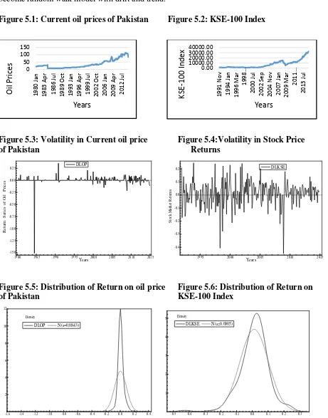
The plots of actual series has drawn to observe the pattern of series and present in the
Figures 5.1 and 5.2.These graphs show actual series of (OP and KSE.100 Index), on monthly
zero mean level. So graphs also show the problem of autocorrelation as well as of
heteroscedasticity. All the three graphs also show increasing trend of the data. So, our model
[image:17.612.74.535.122.709.2]become random walk model with drift and trend.
Figure 5.1: Current oil prices of Pakistan Figure 5.2: KSE-100 Index
[image:17.612.71.268.176.290.2]
Figure 5.3: Volatility in Current oil price Figure 5.4:Volatility in Stock Price
of Pakistan Returns
[image:17.612.78.513.513.710.2]
Figure 5.5: Distribution of Return on oil price Figure 5.6: Distribution of Return on
of Pakistan KSE-100 Index
0 50 100 150
1980 Jan 1983 A
p r 1986 Ju l 1989 O ct
1993 Jan 1996 A
p r 1999 Ju l 2002 O ct
2006 Jan 2009 A
p r 2012 Ju l Oi l Pr ic es Years 0.00 10000.00 20000.00 30000.00 40000.00 1991 N o v
1994 Jan 1996 Mar
1998… 2000 Ju l 2002 S e p 2004 N o v
2007 Jan 2009 Mar
2011… 2013 Ju l K SE -10 0 In d e x Years DLOP
1980 1985 1990 1995 2000 2005 2010 2015
-1.50 -1.25 -1.00 -0.75 -0.50 -0.25 0.00 0.25 Years R et ur
n S
er
ie
s of
Oil
P
ri
ce
s
DLOP DLKSE
1995 2000 2005 2010 2015
-0.4 -0.3 -0.2 -0.1 0.0 0.1 0.2 Years S to ck M ar ke t R et ur ns DLKSE
DLOP N(s=0.0843)
-1.6 -1.4 -1.2 -1.0 -0.8 -0.6 -0.4 -0.2 0.0 0.2 0.4 2 4 6 8 10 12 Density
DLOP N(s=0.0843) DLKSE N(s=0.0905)
-0.5 -0.4 -0.3 -0.2 -0.1 0.0 0.1 0.2 0.3 1
2 3 4 5 Density
Through figures 5.3 and 5.4 it can be noted that series are stationary because mean
reversion behavior. But spread is not same. Volatility clustering is here which defines
heteroscedasticity. There is prolonged period of low volatility and high volatility. In this regard
we can say that periods of high volatility tend to be followed by periods of high volatility and
periods of low volatility are followed by periods of low volatility. This suggest that, there is
autocorrelation problem. So we call it ARCH effect. Because series conditionally depends on its
lags.
Above Figures 5.5 and 5.6 show that distribution is like leptokurtic. These show that
probability of extreme values is higher than normal. So, these are left skewed .It means that
distinct players are active with different preferences in same market. The heavy tails show that
the probability of extreme values are high. There is fluctuation in the data. Series are subject to
leptokurtic.
5.3. Engle’s ARCH Heteroscedasticity Test for return series of KSE and OP
In order to examine the ARCH effect we estimated the regression by OLS and obtain
residuals . Then we applied ARCH LM test on the estimated residuals. The estimated results
are given as following;
… (5.2)
(1.77) (1.72)
The absence of ARCH components is the null hypothesis, for all . The
presence of ARCH components is alternative hypothesis, at least one of the
estimated coefficients must be significant. The test statistic NR² follows 𝜒 distribution
with q degrees of freedom. Chi-square tabulated value is less than the estimated value of NR²
then we reject the null hypothesis and conclude that there is an ARCH effect.
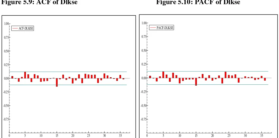
To determine the order of ARIMA we use correlogram for first difference of LOP and
LKSE series. These correlogram show the order of ARIMA for all of them. We used 20 lag
lengths and 95 percent confidence interval for visual inspection. By visual inspection we have
found that there is problem of autocorrelation in series. Because these correlogram are showing
that many spikes lie outside its confidence interval except Dlop which are present in the
Figure 5.7: ACF of Dlop Figure 5.8: PACF of Dlop
Figure 5.9: ACF of Dlkse Figure 5.10: PACF of Dlkse
5.3. The impact of oil price on SPI bivariate E-GARCH model:
This study applies ARIMA BIVARIATE EGARCH (1, 1) model to investigate the
impact of oil price on SPI from the period 1991:M11 to 2014:M12. SPI and oil prices contain
unit root at zero frequency and become stationary at first difference. This model is estimated by
ACF-DLOP
0 5 10 15 20 25 30 35 -0.75
-0.50 -0.25 0.00 0.25 0.50 0.75 1.00
ACF-DLOP PACF-DLOP
0 5 10 15 20 25 30 35 -0.75
-0.50 -0.25 0.00 0.25 0.50 0.75 1.00
PACF-DLOP
ACF-DLKSE
0 5 10 15 20 25 30 35
-0.75 -0.50 -0.25 0.00 0.25 0.50 0.75 1.00
ACF-DLKSE PACF-DLKSE
0 5 10 15 20 25 30 35
-0.75 -0.50 -0.25 0.00 0.25 0.50 0.75 1.00
the Maximum Likelihood Method introduced by Bollerslev and Wooldridge (1992). The results
are presented below (t-statistics in parentheses).
(3.5531) (3.6391) (3.0816) (-3.3597) (-3.8224)
… (5.3a)
(1.2633)
( 𝑡2) = −6.6749 − 0.3111 𝑡2−1 + 0. 013451 𝑡−1 +
(-2.2635) (-0.5130) (0.0837)
0.274067 (| 𝑡−1| − (| 𝑡−1|)) … (5.3 b)
(1.1217)
Diagnostic tests:
ARCH LM Test 𝜒( )= 0.124168 Test of Normality, Jarque.Bera 𝜒( )= 268.77
Autocorrelation Test Q-Statat 1st Lag 𝜒( ) = 0.1260, at 12th Lag 𝜒( )= 15.41
All the diagnostic tests are satisfied the criterion at the 5% level of significance except
the Jarque-Bera test. Conclude that our ARIMA Bivariate EGARCH (1, 1) model has no serial
correlation, no ARCH effect but with non-normal residual. All the estimators of the model are
consistent and significant at the 5% level of significance.
The equation (5.3a) is conditional mean equation of simple Bivariate EGARCH model.
Which reveals that change in SPI is not only affected significantly by its lag but change in oil
prices also plays a significant role in determining the stock price index. We have found positive
relationship between oil prices and SPI. It means SPI is positively affected by oil prices. Thus
any increase in the change in oil prices, indicating increases the change in stock price index.
The equation (5.3b) is conditional variance equation of oil price volatility Bivariate
EGARCH model. News effect SPI asymmetrically that captures by parameter .The size effect
of news reinforce by negative innovation while it is partially effected by a positive innovation. In
our case of Pakistan this have positive value and statistically insignificant at the 5% level of
significance. It means there is no impact of oil price news on SPI. The relative importance
│/ (1+ ). According to them it also measure the differential impact between current conditional variance and own innovation of market. This ratio for Pakistan is 0.97 in our analysis calculated
by above formula.
Generally for the persistent in the volatility shocks is captured by sum of ARCH and
GARCH coefficients. That is near to one (0.97) which also validates in case of Pakistan.
Although these volatility shocks of SPI are very persistent in our case but they are vanished out
overtime.
5.4. The impact of oil price volatility on SPI bivariate E-GARCH model
This study applies ARIMA BIVARIATE EGARCH (1, 1) model is to investigate the
impact of oil price volatility on SPI from the period 1991:M11 to 2014:M12. This model is
estimated by the Maximum Likelihood Method offered by Bollerslev and Wooldridge
(1992).The results are presented below (t-statistics in parentheses).
∆ 𝑡 = −0.012794 + 0.606826∆ 𝑡−15−0.182637 ∆ 𝑡−24 + 0.64645 𝑡−5 − 0.71169 𝑡−15
(-0.718) (7.161) (-2.512) (1.635) (-9.391)
… (5.4a)
(3.845) (1.973)
(-0.925) (56.03) (-1.107)
0.063116 (| 𝑡−1| − (| 𝑡−1|)) … (5.4b)
(0.775)
Diagnostic tests:
ARCH LM Test 𝜒( )= (0.000826) Test of Normality, Jarque Bera𝜒( ) = (274.24)
Autocorrelation Test Q-Stat at 1st Lag 𝜒( )= (0.0008), at 12th Lag𝜒( ) = (17.75)
All the diagnostic tests are satisfied the criterion at the 5% level of significance except
the Jarque Bera test. Conclude that our ARIMA Bivariate EGARCH (1, 1) model has no serial
correlation, no ARCH effect but with non-normal residual. But still all the estimators of the
The equation (5.4a) is conditional mean equation of the impact of oil price volatility on
change in SPI Bivariate EGARCH model. Which reveals that change in SPI is not only affected
significantly by its lag but oil price volatility also plays an important role to determine the SPI.
The nonnegative estimates of conditional variance validates exponential leverage effect rather
quadratic.
The equation (5.4b) is conditional variance equation of oil price volatility Bivariate
EGARCH model. News effect on SPI is asymmetrically that captures by parameter .The size
effect of news reinforce by negative innovation while it is partially effected by a positive
innovation. In our case of Pakistan it has negative value and statistically insignificant. It means
there is no impact of oil price news on SPI. The relative importance formula for positive and
negative news was introduced by Yang and Doong (2004) i.e. │-1+ │/ (1+ ). According to
them it also measure the differential impact between current conditional variance and own
innovation of market.
Generally for the persistent in the volatility shocks is captured by sum of ARCH and
GARCH coefficients. That is one which also validates in case of Pakistan. Although these
volatility shocks of SPI are very persistent in our case but they are vanished out overtime.
6.
Conclusion and Policy Recommendations
Since many years Pakistan is suffering from oil related problems. Because Pakistan is
found to be the major dependent on oil and related products. That is why, it has to spend huge
amount while importing it. According to this point of view, the impact of oil price and its
volatility on Stock market has been analyzed in this study. While some studies have conducted to
examine the impact of energy prices specially oil prices on inflation and other macroeconomics
variables but still there is no study has examined the impact of oil price volatility on Stock
market. In Pakistan, we can see that limited studies were done regarding to this topic. So there is
a gap in literature that impact of oil price volatility on stock market index in Pakistan has not
studied and observed for said relationship. In this study we used the financial time series
econometrics techniques. First applied the Box-Cox transformation on the data. Which suggested
log transformation is required for all series. As data used will be monthly, Beaulieu and Miron
(1992) seasonal unit root test is applied here to test stationarity of the data. All variables contain
unit root at zero frequency and become stationary at first difference. Further to test for the
Granger (1987) two-step method. And finally Bivariate EGARCH model is used to investigate
the impact of oil price volatility on Stock market index. EGARCH Model is presented by Nelson
(1991). According to Nelson this model addressed with the asymmetric effect and relaxed the
restriction of non-negativity and also captures the effect of news on volatility better than
GARCH model. This model is estimated by using Maximum Likelihood Method proposed by
Bollerslev and Woolridge (1992).
We have found positive relationship between oil prices and Stock market Index. It means
SPI is positively affected by oil prices. In case of Pakistan, asymmetric impact is positive but
statistically insignificant at the 5% level of significance. But in the case of oil price volatility
Bivariate EGARCH model, it is negative and statistically insignificant. It means there is no
impact of oil price news on SPI. This study concludes that SPI is positively and significantly
affected by oil price volatility. The sum of ARCH and GARCH coefficients validate these
volatility shocks of SPI are very persistent in our case but they are vanished out overtime.
There are some main points which could be take into consideration from the policy
perspective. These steps are based on the above discussion of results and testing for relationship
between Oil Prices and Stock market. According to this study, Stock market is positively
affected by oil prices. If oil prices are stable then stock market are also stable. Being an oil
importing country, First government can get advantage by increasing their strategic oil reserves
and protect themselves from the risk of supply shortage. Secondly, government would be made
alternative fuels like Coal, natural gas and renewable energy. In order to minimize the oil price
fluctuations which have an adverse impact on our national economy government would improve
References
Ansar, I. and M. Asaghar (2013). "The impact of oil prices on stock exchange and CPI in Pakistan." IOSR Journal of Business and Management (IOSR -JBM). E-ISSN: 32-36.
Beaulieu, J., & Miron, J. (1993). Seasonal unit roots in aggregate U.S. data. Journal of Econometrics 55, 305-328.
Bodenstein,Guerrieri and Kilian (2012). "Monetary policy responses to oil price fluctuations." IMF Economic Review 60(4): 470 -504.
Box, G. E., & Cox, D. R. (1964). An Analysis of Transformations. Journal of the Royal Statistical Society 26, 211-243.
Dhaoui, A. and N. Khraief (2014). Empirical linkage between oil price and stock market returns and volatility: Evidence from international developed markets, Economics Discussion Papers.
Dickey, D. A., and W. A, Fuller (1979) Distribution of Estimators for Time Series Regression with a Unit Root. Journal of the American Statistical Association. vol. 74, pp. 423-431.
Enders, W. (2010). Applied Econometrics Time Series Chapter No. 5.John Wiley & Sons.
Engle, R. F. and C. W. Granger (1987). "Co-integration and error correction: representation, estimation, and testing." Econometrica: journal of the Econometric Society: 251-276.
Fatima, T. and A. Bashir "Oil Price and Stock Market Fluctuations: Emerging Markets (A Comparative Study of Pakistan and China)."International Review of Management and Business Research, Vol.3 (Issue.4) :1958 -1976
Federer, J. (1996). Oil Price Volatility and Macroeconomy. Journal of Macroeconomics, 1–26.
Franses, P. H., and Hobijin, B. (1997), “Critical values for unit root tests in seasonal time
series”, Journal of Applied Statistics, 24(1), 25-48.
Hasan, A. and Z. M. Nasir (2008). "Macroeconomic factors and equity prices: An empirical investigation by using ARDL approach." The Pakistan Development Review: 501-513.
Hamilton, J. D. (1983). Oil and the Macro economy since World War II. Journal of Political Economy , 228-248.
Jawad, M. (2013). "Oil Price Volatility and its Impac t on Economic Growth in Pakistan." Nature 1(4): 62-68.
Jones, C. M. and G. Kaul (1996). "Oil and the stock markets." The Journal of Finance 51(2): 463-491.
Khan, M. A. and A. Ahmed (2011). "Macroeconomic effects of global food and oil price shocks to the Pakistan economy: a structural vector autoregressive (SVAR) analysis." The Pakistan Development Review: 491 -511.
Kiani, A. (2011). "Impact of high oil prices on Pakistan’s economic growth." World
100: 120.
Kilian, L. (2008). "The economic effects of energy price shocks." Journal of Economic Literature: 871-909.
Le, T.-H. and Y. Chang (2011). "The impact of oil price fluctuations on stock markets in developed and emerging economies."Economic Growth Center Working Paper No. 2011/13 http://egc.hss.ntu.edu.sg
Mordi, C. N. and M. A. Adebiyi (2010). "The asymmetric effects of oil price shocks on output and prices in Nigeria using a structural VAR model." Central Bank of Nigeria 48(1): 1-32
Nazir, S. and A. Qayyum (2014). "Impact of Oil Price and Shocks on Economic Growth of Pakistan: Multivariate Analysis."MPRA Paper 55929, University Library of Munich, Germany, revised 2014
Park, J. and R. A. Ratti (2008). "Oil price shocks and stock markets in the US and 13 European countries." Energy Economics 30(5): 2587 -2608.
Qayyum, A. and S. Anwar (2011). "Impact of Monetary Policy on the Volatility of Stock Market in Pakistan."MPRA Paper No.31188, Posted 3.June 2011
http://mpra.ub.uni-muenchen.de/31188/
Qayyum, A. and A. R. Kemal (2006). Volatility Spillover between the Stock Market and the Foreign Market in Pakistan, Pakistan Institute of Development Economics. PIDE Working Papers 2006-7 http://www.pide.org.pk
Rahman, S. and A. Serletis (2011). "The asymmetric effects of oil price shocks." Macroeconomic Dynamics 15(S3): 437-471.