Graph Branch Algorithm: An Optimum Tree Search Method for Scored
Dependency Graph with Arc Co-occurrence Constraints
Hideki Hirakawa
Toshiba R&D Center
1 Komukai Toshiba-cho, Saiwai-ku, Kawasaki 210, JAPAN
Abstract
Various kinds of scored dependency graphs are proposed as packed shared data structures in combination with optimum dependency tree search algorithms. This paper classifies the scored dependency graphs and discusses the specific features of the “Dependency Forest” (DF) which is the packed shared data structure adopted in the “Preference Dependency Grammar” (PDG), and proposes the “Graph Branch Algorithm” for computing the optimum dependency tree from a DF. This paper also reports the experiment showing the computational amount and behavior of the graph branch algorithm.
1 Introduction
The dependency graph (DG) is a packed shared data structure which consists of the nodes corre-sponding to the words in a sentence and the arcs showing dependency relations between the nodes. The scored DG has preference scores attached to the arcs and is widely used as a basis of the opti-mum tree search method. For example, the scored DG is used in Japanese Kakari-uke analysis1 to represent all possible kakari-uke(dependency) trees(Ozeki, 1994),(Hirakawa, 2001). (McDon-ald et al., 2005) proposed a dependency analysis method using a scored DG and some maximum spanning tree search algorithms. In this method, scores on arcs are computed from a set of features obtained from the dependency trees based on the
1Kakari-uke relation, widely adopted in Japanese
sen-tence analysis, is projective dependency relation with a con-straint such that the dependent word is located at the left-hand side of its governor word.
optimum parameters for scoring dependency arcs obtained by the discriminative learning method.
There are various kinds of dependency analy-sis methods based on the scored DGs. This pa-per classifies these methods based on the types of the DGs and the basic well-formed constraints and explains the features of the DF adopted in PDG(Hirakawa, 2006). This paper proposes the graph branch algorithm which searches the opti-mum dependency tree from a DF based on the branch and bound (B&B) method(Ibaraki, 1978) and reports the experiment showing the computa-tional amount and behavior of the graph branch algorithm. As shown below, the combination of the DF and the graph branch algorithm enables the treatment of non-projective dependency analysis and optimum solution search satisfying the single valence occupation constraint, which are out of the scope of most of the DP(dynamic programming)-based parsing methods.
2 Optimum Tree Search in a Scored DG
2.1 Basic Framework
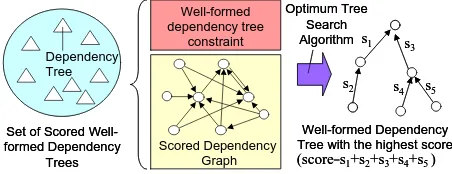
Figure 1 shows the basic framework of the opti-mum dependency tree search in a scored DG. In general, nodes in a DG correspond to words in the sentence and the arcs show some kind of de-pendency relations between nodes. Each arc has
Scored Dependency Graph Dependency
Tree
Set of Scored Well-formed Dependency
Trees
Well-formed dependency tree
constraint
Optimum Tree Search Algorithm
Well-formed Dependency Tree with the highest score
s1
s2 s3
s4 s5
(score=s1+s2+s3+s4+s5 )
Scored Dependency Graph Dependency
Tree
Set of Scored Well-formed Dependency
Trees
Well-formed dependency tree
constraint
Optimum Tree Search Algorithm
Well-formed Dependency Tree with the highest score
s1
s2 s3
s4 s5
[image:1.595.310.536.659.746.2](score=s1+s2+s3+s4+s5 )
Figure 1: The optimum tree search in a scored DG
a preference score representing plausibility of the relation. The well-formed dependency tree con-straint is a set of well-formed concon-straints which should be satisfied by all dependency trees repre-senting sentence interpretations. A DG and a well-formed dependency tree constraint prescribe a set of well-formed dependency trees. The score of a dependency tree is the sum total of arc scores. The optimum tree is a dependency tree with the highest score in the set of dependency trees.
2.2 Dependency Graph
DGs are classified into some classes based on the types of nodes and arcs. This paper assumes three types of nodes, i.e. word-type, WPP-type2 and concept-type3. The types of DGs are called a word DG, a WPP DG and a concept DG, respectively. DGs are also classified into non-labeled and la-beled DGs. There are some types of arc labels such as syntactic label (ex. “subject”,“object”) and semantic label (ex. “agent”,“target”). Var-ious types of DGs are used in existing sys-tems according to these classifications, such as non-label word DG(Lee and Choi, 1997; Eisner, 1996; McDonald et al., 2005)4, syntactic-label word DG (Maruyama, 1990), semantic-label word DG(Hirakawa, 2001), non-label WPP DG(Ozeki, 1994; Katoh and Ehara, 1989), syntactic-label WPP DG(Wang and Harper, 2004), semantic-label concept DG(Harada and Mizuno, 2001).
2.3 Well-formedness Constraints and Graph Search Algorithms
There can be a variety of well-formedness con-straints from very basic and language-independent constraints to specific and language-dependent constraints. This paper focuses on the following four basic and language-independent constraints which may be embedded in data structure and/or the optimum tree search algorithm.
(C1) Coverage constraint: Every input word has a corresponding node in the tree
(C2) Single role constraint(SRC): No two nodes in a dependency tree occupy the same input position
2
WPP is a pair of a word and a part of speech (POS). The word “time” has WPPs such as “time/n” and “time/v”.
3One WPP (ex. “time/n”) can be categorized into one or
more concepts semantically (ex. “time/n/period time” and “time/n/clock time”).
4This does not mean that these algorithms can not handle
labeled DGs.
(C3) Projectivity constraint(PJC): No arc crosses another arc5
(C4) Single valence occupation constraint(SVOC): No two arcs in a tree occupy the same valence of a predicate
(C1) and (C2), collectively referred to as “cover-ing constraint”, are basic constraints adopted by almost all dependency parsers. (C3) is adopted by the majority of dependency parsers which are called projective dependency parsers. A projective dependency parser fails to analyze non-projective sentences. (C4) is a basic constraint for valency but is not adopted by the majority of dependency parsers.
Graph search algorithms, such as the Chu-Liu-Edmonds maximum spanning tree algorithm (Chu and Liu, 1965; Edmonds, 1967), algorithms based on the dynamic programming (DP) princi-ple (Ozeki, 1994; Eisner, 1996) and the algorithm based on the B&B method (Hirakawa, 2001), are used for the optimum tree search in scored DGs. The applicability of these algorithms is closely re-lated to the types of DGs and/or well-formedness constraints. The Chu-Liu-Edmonds algorithm is very fast (O(n
2
) for sentence length n), but it
works correctly only on word DGs. DP-based al-gorithms can satisfy (C1)-(C3) and run efficiently, but seems not to satisfy (C4) as shown in 2.4.
(C2)-(C4) can be described as a set of co-occurrence constraints between two arcs in a DG. As described in Section 2.6, the DF can represent (C2)-(C4) and more precise constraints because it can handle co-occurrence constraints between two arbitrary arcs in a DG. The graph branch algorithm described in Section 3 can find the optimum tree from the DF.
2.4 SVOC and DP
(Ozeki and Zhang, 1999) proposed the minimum cost partitioning method (MCPM) which is a parti-tioning computation based on the recurrence equa-tion where the cost of joining two partiequa-tions is the cost of these partitions plus the cost of com-bining these partitions. MCPM is a generaliza-tion of (Ozeki, 1994) and (Katoh and Ehara, 1989) which compute the optimum dependency tree in a scored DG. MCPM is also a generalization of the probabilistic CKY algorithm and the Viterbi
algo-5Another condition for projectivity, i.e. “no arc covers top
agent1,15 Isha-mo (doctor) Wakaranai (not_know) Byouki-no (sickness) Kanja (patient) target2,10 agent3,5 target4,7 in-state7,10 agent5,15 target6,5
OS1[15]: (agent1,15)
OS3[22]: (agent1,15) + (target4,7)
OS2[10]: (in-state7,10)
OS4[25]: (agent5,15) + (in-state7,10) NOS1[10]: (target2,10)
NOS2[20]: (target4,10) + (in-state7,10) OS1[15]: (agent1,15)
OS4[25]: (agent5,15) + (in-state7,10)
Well-formed optimum solutions for covering whole phrase agent1,15 Isha-mo (doctor) Wakaranai (not_know) Byouki-no (sickness) Kanja (patient) target2,10 agent3,5 target4,7 in-state7,10 agent5,15 target6,5
OS1[15]: (agent1,15)
OS3[22]: (agent1,15) + (target4,7)
OS2[10]: (in-state7,10)
OS4[25]: (agent5,15) + (in-state7,10) NOS1[10]: (target2,10)
NOS2[20]: (target4,10) + (in-state7,10) OS1[15]: (agent1,15)
OS4[25]: (agent5,15) + (in-state7,10)
[image:3.595.78.284.60.216.2]Well-formed optimum solutions for covering whole phrase
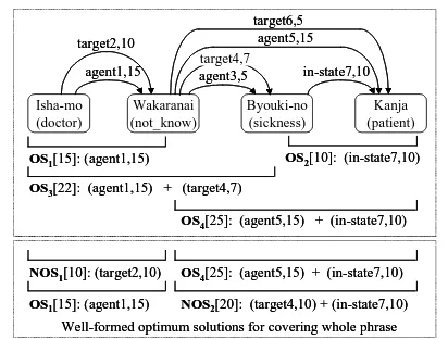
Figure 2: Optimum tree search satisfying SVOC
[image:3.595.310.524.62.236.2]rithm6. The minimum cost partition of the whole sentence is calculated very efficiently by the DP principle. The optimum partitioning obtained by MCPM constitutes a tree covering the whole sen-tence satisfying the SRC and PJC. However, it is not assured that the SVOC is satisfied by MCPM.
Figure 2 shows a DG for the Japanese phrase “Isha-mo Wakaranai Byouki-no Kanja” encom-passing dependency trees corresponding to “a pa-tient suffering from a disease that the doctor doesn’t know”, “a sick patient who does not know the doctor”, and so on.OS
1 -OS
4represent the
op-timum solutions for the phrases specified by their brackets computed based on MCPM. For exam-ple,OS
3gives an optimum tree with a score of 22
(consisting ofagent1andtarget4) for the phrase
“Isha-mo Wakaranai Byouki-no”. The optimum solution for the whole phrase is eitherOS
1 +OS 4 orOS 3 +OS
2due to MCPM. The former has the
highest score 40(= 15+25) but does not satisfy
the SVOC because it has agent1 and agent5
si-multaneously. The optimum solutions satisfying the SVOC areNOS
1 +OS
4 and OS
1
+NOS 2
shown at the bottom of Figure 2. NOS 1 and NOS
2 are not optimum solutions for their word
coverages. This shows that it is not assured that MCPM will obtain the optimum solution satisfy-ing the SVOC.
On the contrary, it is assured that the graph branch algorithm computes the optimum solu-tion(s) satisfying the SVOC because it com-putes the optimum solution(s) satisfying any co-occurrence constraints in the constraint matrix. It is an open problem whether an algorithm based on the DP framework exists which can handle the SVOC and arbitrary arc co-occurrence constraints.
6Specifically, MTCM corresponds to probabilistic CKY
and the Viterbi algorithm because it computes both the opti-mum tree score and its structure.
Constraint Matrix
Dependency Graph
Meaning of Arc Name sub : subject obj : object npp : noun-preposition vpp : verb-preposition pre : preposition nc : noun compound det : determiner rt : root
npp19 det14 pre15 vpp20 vpp18 sub24 sub23 obj4
nc2 obj16
0,time/n 1,fly/v 0,time/v 1,fly/n 2,like/p 2,like/v 3,an/det 4,arrow/n root rt29 rt32 rt31 Constraint Matrix Dependency Graph
Meaning of Arc Name sub : subject obj : object npp : noun-preposition vpp : verb-preposition pre : preposition nc : noun compound det : determiner rt : root
npp19 det14 pre15 vpp20 vpp18 sub24 sub23 obj4
nc2 obj16
0,time/n 1,fly/v 0,time/v 1,fly/n 2,like/p 2,like/v 3,an/det 4,arrow/n root rt29 rt32 rt31
Meaning of Arc Name sub : subject obj : object npp : noun-preposition vpp : verb-preposition pre : preposition nc : noun compound det : determiner rt : root
npp19 det14 pre15 vpp20 vpp18 sub24 sub23 obj4
nc2 obj16
0,time/n 1,fly/v 0,time/v 1,fly/n 2,like/p 2,like/v 3,an/det 4,arrow/n root rt29 rt32 rt31 npp19 det14 pre15 vpp20 vpp18 sub24 sub23 obj4
nc2 obj16
0,time/n 1,fly/v 0,time/v 1,fly/n 2,like/p 2,like/v 3,an/det 4,arrow/n root rt29 rt32 rt31 npp19 det14 pre15 vpp20 vpp18 sub24 sub23 obj4
nc2 obj16
0,time/n 1,fly/v 0,time/v 1,fly/n 2,like/p 2,like/v 3,an/det 4,arrow/n root rt29 rt32 rt31
Figure 3: Scored dependency forest
2.5 Semantic Dependency Graph (SDG)
The SDG is a semantic-label word DG designed for Japanese sentence analysis. The optimum tree search algorithm searches for the optimum tree satisfying the well-formed constraints (C1)-(C4) in a SDG(Hirakawa, 2001). This method is lack-ing in terms of generality in that it cannot handle backward dependency and multiple WPP because it depends on some linguistic features peculiar to Japanese. Therefore, this method is inherently in-applicable to languages like English that require backward dependency and multiple POS analysis. The DF described below can be seen as the ex-tension of the SDG. Since the DF has none of the language-dependent premises that the SDG has, it is applicable to English and other languages.
2.6 Dependency Forest (DF)
The DF is a packed shared data structure en-compassing all possible dependency trees for a sentence adopted in PDG. The DF consists of a dependency graph (DG) and a constraint matrix (CM). Figure 3 shows a DF for the example sen-tence “Time flies like an arrow.” The DG consists of nodes and directed arcs. A node represents a WPP and an arc shows the dependency relation between nodes. An arc has its ID and preference score. CM is a matrix whose rows and columns are a set of arcs in DG and prescribes the co-occurrence constraint between arcs. Only when CM(i,j) is○,ar
i and ar
j are co-occurrable in
one dependency tree.
The generated CM assures that the parse trees in the parse forest and the dependency trees in the DF have mutual correspondence(Hirakawa, 2006). CM can represent (C2)-(C4) in 2.3 and more pre-cise constraints. For example, PDG can generate a DF encompassing non-projective dependency trees by introducing the grammar rules defining non-projective constructions. This is called the controlled non-projectivity in this paper. Treat-ment of non-projectivity as described in (Kanahe et al., 1998; Nivre and Nilsson, 2005) is an impor-tant topic out of the scope of this paper.
3 The Optimum Tree Search in DF
This section shows the graph branch algorithm based on the B&B principle, which searches for the optimum well-formed tree in a DF by apply-ing problem expansions called graph branchapply-ing.
3.1 Outline of B&B Method
The B&B method(Ibaraki, 1978) is a principle for solving computationally hard problems such as NP-complete problems. The basic strategy is that the original problem is decomposed into eas-ier partial-problems (branching) and the original problem is solved by solving them. Pruning called a bound operation is applied if it turns out that the optimum solution to a partial-problem is inferior to the solution obtained from some other partial-problem (dominance test)7, or if it turns out that a partial-problem gives no optimum solutions to the original problem (maximum value test). Usu-ally, the B&B algorithm is constructed to mini-mize the value of the solution. The graph branch algorithm in this paper is constructed to maximize the score of the solution because the best solution is the maximum tree in the DF.
3.2 Graph Branch Algorithm
The graph branch algorithm is obtained by defin-ing the components of the original B&B skeleton algorithm, i.e. the partial-problem, the feasible so-lution, the lower bound value, the upper bound value, the branch operation, and so on(Ibaraki, 1978). Figure 4 shows the graph branch algorithm which has been extended from the original B&B skeleton algorithm to search for all the optimum trees in a DF. The following sections explain the B&B components of the graph branch algorithm.
7The dominance test is not used in the graph branch
algo-rithm.
!
" #$% " &% " #$%
'( " ) * !% ' +
,* - ,!
"" #$! # ) . %$
# " * !% $
/ , 0 + , 1 + 2( " , 0! 3
02(! " ) *4 !%
+ , 3
0 "" * ! # ) *% $ 5 + ! 2( , 6
+ + 3
2( 7 ! # " 2(% " #0$% $
8 + !
'( 9 ! #) *% $
/ 23
2 " ) * !%
1 + ! , + . ), , 3
2( : '(! # (/2 " 2%) ,% $
21 + ; + "7
2( "" '(! #
" #0$ < % ++ , 0
= , !
! .
2 >" #$! #(/2 " 2%) ,% $ ! .
(/2 " *1 ,* 0!%
(/2 >" #$! #) ,% $
# ) *%$ $
, ? ,) !
@ ,+ + (/2
/,+2 " ),*, (/2!% " ' /, +2 & #$
%
) ,* %
* A !
" & #$% ) ,* %
. B !
"" &! # , $
#C DE FEGHIJHK G ILHDMNM EIONHDIPE $
Figure 4: Graph branch algorithm
(1) Partial-problem
Partial-problem P
i in the graph branch
algo-rithm is a problem searching for all the well-formed optimum trees in a DFDF
i consisting of
the dependency graphDG
i and constraint matrix
CM i.
P
i consists of the following elements.
(a) Dependency graphDG i
(b) Constraint matrixCM i
(c) Feasible solution valueLB i
(d) Upper bound valueUB i
(e) Inconsistent arc pair listIAPL i
The constraint matrix is common to all partial-problems, so one CM is shared by all
partial-problems.DG
iis represented by “
rem[::℄” which
shows a set of arcs to be removed from the whole dependency graphDG. For example, “rem[b;d℄”
represents a partial dependency graph [a;;e℄ in
the caseDG = [a;b;;d;e℄. IAPL
i is a list of
(2) Algorithm for Obtaining Feasible Solution and Lower Bound Value
In the graph branch algorithm, a well-formed dependency tree in the dependency graph DGof
the partial-problem P is assigned as the feasible
solutionFSofP
8. The score of the feasible
solu-tionFSis assigned as the lower bound valueLB.
The function for computing these valuesget fsis
called a feasible solution/lower bound value func-tion. The details are not shown due to space lim-itations, but get fsis realized by the
backtrack-based depth-first search algorithm with the opti-mization based on the arc scores. get fsassures
that the obtained solution satisfies the covering constraint and the arc co-occurrence constraint. The incumbent value z (the best score so far) is
replaced by theLBatS3in Figure 4 if needed.
(3) Algorithm for Obtaining Upper Bound
Given a set of arcsAwhich is a subset ofDG,
if the set of dependent nodes9of arcs inAsatisfies
the covering constraint, the arc setAis called the
well-covered arc set. The maximum well-covered arc set is defined as a well-covered arc set with the highest score. In general, the maximum well-covered arc set does not satisfy the SRC and does not form a tree. In the graph branch algorithm, the score of the maximum well-covered arc set of a de-pendency graphGis assigned as the upper bound
valueUBof the partial-problemP. Upper bound
functionget ubcalculatesUBby scanning the arc
lists sorted by the surface position of the depen-dent nodes of the arcs.
(4) Branch Operation
Figure 5 shows a branch operation called a graph branch operation. Child partial-problems of
P are constructed as follows:
(a) Search for an inconsistent arc pair(ar i
;ar j
)
in the maximum well-covered arc set of the DG ofP.
(b) Create child partial-problemsP i,
P
jwhich
have new DGsDG i
=DG far
j gand
DG j
=DG far
i
grespectively.
Since a solution to P cannot have both ar i and
ar
jsimultaneously due to the co-occurrence
con-straint, the optimum solution of P is obtained
from either/both P
i or/and P
j. The child
partial-8A feasible solution may not be optimum but is a possible
interpretation of a sentence. Therefore, it can be used as an approximate output when the search process is aborted.
9The dependent node of an arc is the node located at the
source of the arc.
DG: Dependency graph of parent problem
arcj
arci
DGj: Dependency graph
for child problem Pj
arcj
DGi: Dependency graph
for child problem Pi
arci
Remove arcj Remove arci
DG: Dependency graph of parent problem
arcj
arci
arcj
arci
DGj: Dependency graph
for child problem Pj
arcj
arcj
DGi: Dependency graph
for child problem Pi
arci
arci
Remove arcj Remove arci
Figure 5: Graph branching
problem is easier than the parent partial-problem because the size of the DG of the child partial-problem is less than that of its parent.
In Figure 4,get iaplcomputes the list of
incon-sistent arc pairsIAPL(Inconsistent Arc Pair List)
for the maximum well-covered arc set ofP i. Then
the graph branch function graph branh selects
one inconsistent arc pair(ar i
;ar j
)fromIAPL
for branch operation. The selection criteria for
(ar i
;ar j
)affects the efficiency of the algorithm.
graph branh selects the inconsistent arc pair
containing the highest score arc inBACL(Branch
Arc Candidates List). graph branh calculates
the upper bound value for a child partial-problem byget uband sets it to the child partial-problem.
(5) Selection of Partial-problem
selet problememploys the best bound search
strategy, i.e. it selects the partial-problem which has the maximum bound value among the active partial-problems. It is known that the number of partial-problems decomposed during computation is minimized by this strategy in the case that no dominance tests are applied (Ibaraki, 1978).
(6) Computing All Optimum Solutions
In order to obtain all optimum solutions, partial-problems whose upper bound values are equal to the score of the optimum solution(s) are expanded at S8 in Figure 4. In the case that at least one
inconsistent arc pair remains in a partial-problem (i.e. IAPL6=fg), graph branch is performed
based on the inconsistent arc pair. Otherwise, the obtained optimum solution FS is checked if
one of the arcs in FS has an equal rival arc by
arswith alternatives function. The equal
ri-val arc of arcAis an arc whose position and score
are equal to those of arcA. If an equal rival arc
of an arc in FS exists, a new partial-problem is
generated by removing the arc inFS. S8assures
P0 P1 P3 P2 P4 ! " # $ !# $ %&' ( " # $ %&' ( ! " # $ !# $ %&' ( " # $ %&' ( %&'( " # $ %&'( P0 P1 P3 P2 P4 ! " # $ !# $ %&' ( " # $ %&' ( ! " # $ !# $ %&' ( " # $ %&' ( %&'( " # $ %&'(
Figure 6: Search diagram
greater than or equal to the score of the optimum solutions when the computation stopped.
4 Example of Optimum Tree Search
This section shows an example of the graph branch algorithm execution using the DF in Fig.3.
4.1 Example of Graph Branch Algorithm
The search process of the B&B method can be shown as a search diagram constructing a partial-problem tree representing the parent-child relation between the partial-problems. Figure 6 is a search diagram for the example DF showing the search process of the graph branch algorithm.
In this figure, boxP
i is a partial-problem with
its dependency graph rem, upper bound value
UB, feasible solution and lower bound valueLB
and inconsistent arc pair listIAPL. SuffixiofP i
indicates the generation order of partial-problems. Updating of global variable z (incumbent value)
and O (set of incumbent solutions) is shown
un-der the box. The value of the left-hand side of the arrow is updated to that of right-hand side of the arrow during the partial-problem processing. De-tails of the behavior of the algorithm in Figure 4 are described below.
In S1(initialize), z, O and AP are set to
1, fg and fP 0
g respectively. The DG of P 0 is
that of the example DF. This is represented by
rem = [℄. get ub sets the upper bound value
(=63) of P 0 to
UB. In practice, this is
calcu-lated by obtaining the maximum well-covered arc set ofP
0. In
S2(searh),seletproblemselects
P 0 and
get fs(P 0
)is executed. The feasible
so-lution FS and its score LB are calculated to set
FS = [14;2;16;23;29℄, LB = 50 (P
0 in the
search diagram). S3(inumbent value update)
updates z and O to new values. Then,
get iapl(P 0
) computes the inconsistent arc pair
list [(2;15);(15;23);(2 3;18 );( 2;18 )℄ from the
maximum well-covered arc set [14;2;15;23;18℄
and set it to IAPL. S5(maximumvaluetest)
compares the upper bound valueUBand the
fea-sible solution valueLB. In this case,LB <UB
holds, soBACLis assigned the value of IAPL.
The next stepS6(branhoperation)executes the
graph branh function. graph branh selects
the arc pair with the highest arc score and performs the graph branch operation with the selected arc pair. The following is a BACLshown with the
arc names and arc scores.
[(n2[17℄;pre15[10℄);(pre15[1 0℄;sub23[ 10℄ );
(sub23[10℄;vpp18[9℄);(n2[1 7℄ ;vpp18 [9℄ )℄
Scores are shown in [ ℄. The arc pair
contain-ing the highest arc score is (2;15) and (2;18)
containing n2[17℄. Here, (2;15) is selected and
partial-problemsP 1
(rem[2℄)andP 2
(rem[15℄)are
generated. P
0 is removed from
AP and the new
two partial-problems are added toAP resulting in
AP = fP 1
;P 2
g. Then, based on the best bound
search strategy,S2(searh)is tried again.
P
1 updates
z and O because P
1 obtained a
feasible solution better than that in O obtained
by P 0.
P 2 and
P
4 are terminated because they
have no feasible solution. P
3 generates a
feasi-ble solution but z and O are not updated. This
is because the obtained feasible solution is infe-rior to the incumbent solution inO. The optimum
solution(=f[14;24;15;31 ;1 8℄g) is obtained byP 1.
The computation from P 2 to
P
4 is required to
as-sure that the feasible solution ofP
1is optimum.
5 Experiment
This section describes some experimental results showing the computational amount of the graph branch algorithm.
5.1 Environment and Performance Metric
An existing sentence analysis system10(called the
oracle system) is used as a generator of the test corpus, the preference knowledge source and the correct answers. Experiment data of 125,320 sen-tences11 extracted from English technical
docu-10A real-world rule-based machine translation system with
a long development history
11Sentences ending with a period and parsable by the
ments is divided into open data (8605 sentences) and closed data (116,715 sentences). The prefer-ence score source, i.e. the WPP frequencies and the dependency relation frequencies are obtained from the closed data. The basic PDG grammar (907 extended CFG rules) is used for generating the DFs for the open data.
The expanded problem number (EPN), a prin-cipal computational amount factor of the B&B method, is adopted as the base metric. The fol-lowing three metrics are used in this experiment.
(a) EPN in total (EPN-T): The number of the ex-panded problems which are generated in the entire search process.
(b) EPN for the first optimum solution (EPN-F): The number of the expanded problems when the first optimum solution is obtained.
(c) EPN for the last optimum solution (EPN-L): The number of the expanded problems when the last optimum solution is obtained. At this point, all optimum solutions are obtained.
Optimum solution number (OSN) for a problem, i.e. the number of optimum dependency trees in a given DF, gives the lower bound value for all these metrics because one problem generates at most one solution. The minimum value of OSN is 1 because every DF has at least one dependency tree. As the search process proceeds, the algorithm finds the first optimum solution, then the last opti-mum solution, and finally terminates the process by confirming no better solution is left. There-fore, the three metrics and OSN have the relation OSNEPN-FEPN-LEPN-T. Average
val-ues for these are described as Ave:OSN, Ave:EPN-F, Ave:EPN-L and Ave:EPN-T.
5.2 Experimental Results
An evaluation experiment for the open data is performed using a prototype PDG system imple-mented in Prolog. The sentences containing more than 22 words are neglected due to the limita-tion of Prolog system resources in the parsing pro-cess. 4334 sentences out of the remaining 6882 test sentences are parsable. Unparsable sentences (2584 sentences) are simply neglected in this ex-periment. The arc precision ratio12 of the oracle
12Correct arc ratio with respect to arcs in the output
depen-dency trees (Hirakawa, 2005).
!"#$% &'()*+ ,,
!"#.%&'()/+01
!"#2
%&'()/+3*-45"%&'()/+/6
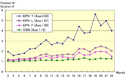
-Figure 7: EPN-T, EPN-F EPN-F and OSN
system for 136 sentences in this sentence set is 97.2% with respect to human analysis results.
All optimum trees are computed by the graph branch algorithm described in Section 3.2. Fig-ure 7 shows averages of EPN-T, EPN-L, EPN-F and OSN with respect to sentence length. Over-all averages of EPN-T, EPN-L, EPN-F and OSN for the test sentences are 3.0, 1.67, 1.43 and 1.15. The result shows that the average number of prob-lems required is relatively small. The gap between Ave:EPN-T and Ave:EPN-L (3.0-1.67=1.33) is much greater than the gap between Ave:EPN-L and Ave:OSN(1.67-1.15=0.52). This means that the major part of the computation is performed only for checking if the obtained feasible solutions are optimum or not.
According to (Hirakawa, 2001), the experiment on the B&B-based algorithm for the SDG shows the overall averages of T, AVE:EPN-F are 2.91, 1.33 and the average CPU time is 305.8ms (on EWS). These values are close to those in the experiment based on the graph branch algorithm. Two experiments show a tendency for the optimum solution to be obtained in the early stage of the search process. The graph branch al-gorithm is expected to obtain the comparable per-formance with the SDG search algorithm.
(Hirakawa, 2001) introduced the improved up-per bound function g’(P) into the B&B-based al-gorithm for the SDG and found Ave:EPN-T is re-duced from 2.91 to 1.82. The same technique is introduced to the graph branch algorithm and has obtained the reduction of the Ave:EPN-T from 3.00 to 2.68.
[image:7.595.310.527.50.195.2]
!
!
" !
[image:8.595.83.287.56.194.2]" #$%&' !
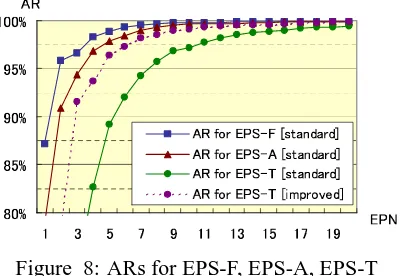
Figure 8: ARs for EPS-F, EPS-A, EPS-T
tion and the last optimum solution to whole sen-tences with respect to the EPNs. This kind of ratio is called an achievement ratio (AR) in this paper. From Figure 8, the ARs for T, L, EPN-F (plotted in solid lines) are 97.1%,99.6%,99.8% respectively at the EPN 10. The dotted line shows the AR for EPN-T of the improved algorithm us-ing g’(P). The use of g’(P) increases the AR for EPN-T from 97.1% to 99.1% at the EPN 10. How-ever, the effect of g’(P) is quite small for EPN-F and EPN-L. This result shows that the pruning strategy based on the EPN is effective and g’(P) works for the reduction of the problems generated in the posterior part of the search processes.
6 Concluding Remarks
This paper has described the graph branch algo-rithm for obtaining the optimum solution for a DF used in PDG. The well-formedness depen-dency tree constraints are represented by the con-straint matrix of the DF, which has flexible and precise description ability so that controlled non-projectivity is available in PDG framework. The graph branch algorithm assures the search for the optimum trees with arbitrary arc co-occurrence constraints, including the SVOC which has not been treated in DP-based algorithms so far. The experimental result shows the averages of EPN-T, EPN-L and EPN-F for English test sentences are 3.0, 1.67 and 1.43, respectively. The practi-cal code implementation of the graph branch algo-rithm and its performance evaluation are subjects for future work.
References
Y. J. Chu and T. H. Liu. 1965. On the shortest arbores-cence of a directed graph. Science Sinica, 14.
J. Edmonds. 1967. Optimum branchings. Journal
of Research of the National Bureau of Standards,
71B:233–240.
J. Eisner. 1996. Three new probabilistic models for de-pendency parsing: An exploration. In Proceedings
of COLING’96, pages 340–345.
M. Harada and T. Mizuno. 2001. Japanese semantic analysis system sage using edr (in japanese).
Trans-actions of JSAI, 16(1):85–93.
H. Hirakawa. 2001. Semantic dependency analysis method for japanese based on optimum tree search algorithm. In Proceedings of the PACLING2001.
H. Hirakawa. 2005. Evaluation measures for natural language analyser based on preference dependency grammar. In Proceedings of the PACLING2005.
H. Hirakawa. 2006. Preference dependency grammar and its packed shared data structure ’dependency forest’ (in japanese). To appear in Natural Lan-guage Processing, 13(3).
T. Ibaraki. 1978. Branch-and-bounding procedure and state-space representation of combinatorial opti-mization problems. Information and Control, 36,1-27.
S. Kanahe, A. Nasr, and O. Rambow. 1998. Pseudo-projectivity: A polynomially parsable non-projective dependency grammar. In
COLING-ACL’98, pages 646–52.
N. Katoh and T. Ehara. 1989. A fast algorithm for dependency structure analysis (in japanese). In
Pro-ceedings of 39th Annual Convention of the Informa-tion Processing Society.
S. Lee and K. S. Choi. 1997. Reestimation and best-first parsing algorithm for probablistic dependency grammars. In Proceedings of the Fifth Workshop on
Very Large Corpora, pages 41–55.
H. Maruyama. 1990. Constraint dependency grammar and its weak generative capacity. Computer
Soft-ware.
R. McDonald, F. Pereira, K. Ribarov, and J. Hajic. 2005. Non-projective dependency parsing using spanning tree algorithms. In Proceedings of
HLT-EMNLP, pages 523–530.
J. Nivre and J. Nilsson. 2005. Pseudo-projective de-pendency parsing. In ACL-05, pages 99–106.
K. Ozeki and Y. Zhang. 1999. 最小コスト分割問題
としての係り受け解析. In Proceeding of the
Work-shop of The Fifth Annual Meeting of The Association for Natural Language Processing, pages 9–14.
K. Ozeki. 1994. Dependency structure analysis as combinatorial optimization. Information Sciences, 78(1-2):77–99.
W. Wang and M. P. Harper. 2004. A statistical con-straint dependency grammar (cdg) parser. In