The Agreement Measure γcat a Complement to γ Focused on Categorization of a Continuum

γ

Focused on Categorization of a Continuum

Yann Mathet

Universit´e de Caen Normandie GREYC-CNRS

Agreement on unitizing, where several annotators freely put units of various sizes and categories on a continuum, is difficult to assess because of the simultaneaous discrepancies in positioning and categorizing. The recent agreement measureγoffers an overall solution that simultaneously takes into account positions and categories. In this article, I propose the additional coefficient

γ_cat, which complementsγby assessing the agreement on categorization of a continuum, putting aside positional discrepancies. When applied to pure categorization (with predefined units),γ_cat

behaves the same way as the famous dedicated Krippendorff’sα, even with missing values, which proves its consistency. A variation ofγ_catis also proposed that provides an in-depth assessment of categorizing for each individual category. The entire family ofγcoefficients is implemented in free software.

1. Introduction

Agreement measures are commonly used in computational linguistics to assess the reli-ability of annotation processes, in particular in the case of categorization of predefined items, with well-known chance corrected coefficients such asπ(Scott 1955),κ(Cohen 1960, 1968), K-Fleiss (Fleiss 1971), orα(Krippendorff 1980, 2013). However, when deal-ing with unitizdeal-ing, where annotators have to put units of different sizes and categories on a continuum (text, audio, video) by themselves, fewer agreement measures are available and popular. Fortunately, Krippendorff has paved the way since 1995 with the first chance-corrected dedicated measures, from the firstαU(Krippendorff 1995) to a whole family of five coefficients for unitizing (Krippendorff et al. 2016), denoted as theαshereafter.

Recently, Mathet, Widl ¨ocher, and M´etivier (2015) introduced the new coefficient γ, which relies on different assumptions from theαsand thus better corresponds to computational linguistics annotation efforts. In particular, whereas αs rely on the number of intersections between any pair of units from different annotators,γbuilds and relies on an alignment between units that ultimately says which unit from one annotator corresponds to which unit from another annotator, if any. In simple words, γis designed for tasks for which the very notion is unit rather than occupied space: A unit is considered as a whole (i.e., a contiguous entity), not just a portion of the

∗Universit´e de Caen Normandie, UMR 6072 GREYC, F-14032 Caen, France. E-mail:

[email protected].

Submission received: 30 May 2016; revised version received: 12 December 2016; accepted for publication: 10 April 2017.

continuum, and small units are as important as large ones. Moreover, γ is the only measure that copes with overlapping units (intersecting or even nested units). It has also been demonstrated by Mathet, Widl ¨ocher, and M´etivier that γ shows a more homogeneous behavior through different kinds of disagreement (position, category, false positive, false negative) than other methods.

However,γis an overall coefficient for all unitizing discrepancies at the same time. When its value is close to 1, annotations can be trusted as reliable, but when that is not the case, this coefficient does not provide an insight into the kind(s) of discrepancy(ies) between annotators: We know the annotations are not reliable, but we do not know what to focus on to improve them.

This article provides an additional coefficent toγ, namedγ_cat, which focuses on the categorizing part of disagreement between annotators, leaving aside, as much as possible, the unitizing part (in particular, positional discrepancies). In simple words,γ_cat tries to answer the question:If annotators had not had to unitize the continuum (put units by themselves and categorize them), but only to categorize predefined units on the continuum, what would have been their agreement? It shares the same goal as cuα, the measure belonging to theαsdedicated to categorization of a continuum, but relies on the same assumptions asγ. In particular, it shares the same alignment method, before it does a specific computation focused on categories.

In addition, an even more in-depth coefficient, namedγk, is provided that focuses on the agreement on each individual category. It helps to know if a low or moderateγ_cat value comes from discrepancies on some particular categories, and so may be useful in order to modify the annotation model or to enhance the annotation instructions. This additional coefficient corresponds to the recentkαfrom Krippendorff et al. (2016), which replaces a first attempt (Krippendorff 2004).

Section 2 introduces the main requirements for a measure for categorization of a continuum for computational linguistics efforts: Insensitivity to positional discre-pancies; insensivity to false positives/negatives; and insensitivity to size of units.

Section 3 addresses the question of how best to cope with missing values in cate-gorization tasks (when an annotator does not categorize an item whereas some others do), which is a more general (and rarely discussed) question concerning any measure. It will also constitute an additional requirement forγ_cat.

Section 4 explains the design of γ_cat and γ_k in two main steps: First, it uses the aligning procedure ofγ; second, it makes a special computation based on the alignment but focused on categories (or on a given category in the case ofγk). To finish,γ_catandγ_k are benchmarked and compared with the correspondingαsin Section 5. The software is introduced in Section 6.

2. Main Requirements: What Should a Categorial Measure Account For?

In this section, we will see howγ_cat should complement γ. The very objective is that γ_catbe insensitive to disagreements that involve other aspects of unitizing than catego-rization (positions, lengths, etc.), contrary toγ. All the points introduced subsequently are benchmarked in section 5.

2.1 Positional Discrepancies Should Not Impact Categorial Agreement

1 annotator A

annotator B 4

1

2

2 4

1-1 4-1 4-4 4-2 2-2

1-1 4-4

2-2 (alignments)

(intersections)

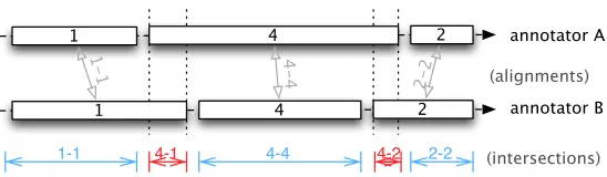
Figure 1

Positional discrepancies but perfect agreement on categories.

but it is not straightforward with unitizing. Figure 1 shows a case of perfect agreement on categories that comes with some disagreement on positions: Both annotators have identified three units at about, but not exactly, the same positions, and totally agree on categorizing these units (respectively, with category “1,” “4,” and “2”). Hence, a mea-sure focused on categorization should provide total agreement in such a configuration. However, measures based on intersections, like the αs, or on atomization of the continuum (a workaround method discussed later), will find a part of the continuum with categorial disagreement, since there is an intersection between units of categories “4” and “1,” and between units of categories “4” and “2.” This is reported at the bottom of Figure 1: There are five intersections, three of them corresponding to correct com-parisons, and two of them corresponding to unfortunate comparisons. This leads here to about 20% fake categorial disagreement, according to corresponding intersection lengths.

What a categorial measure should do here is to compare each unit from annotator A to the corresponding one from annotator B (if any), as reported in Figure 1 by the three gray arrows “1-1,” “4-4,” and “2-2,” and assess here a total agreement. This is typically what theγfamily is designed to do, thanks to its alignment capability.

2.2 False Negatives/Positives Should Not Impact Categorial Agreement

We have to be cautious concerning the terminology. A false negative occurs when an annotator fails to put a unit where she should, namely, where the reference (if any) tells us there should be a unit, and a false positive is the opposite situation. However, no reference exists in the case of agreement measures, and there is a symmetry between false positives and false negatives: If annotator 1 puts a unit where annotator 2 doesn’t, it is a false positive if we consider annotator 2 as the reference, or a false negative if we consider annotator 1 as the reference. However, to make this discussion more simple, we will extend the meaning of false positives/negatives to the field of agreement measures. Here again, such disagreements should not be taken into account by a measure fo-cused on categorization. For instance, such a measure should provide a total agreement if annotator A identifies and categorizes 100 units, and annotator B identifies only 50 of them but agrees with A on categories.

2.3 Length of Units Should Not Be Taken Into Account

Barack Hussein Obama II is the 44th and current (…). In 2004, Obama received national (…)

Barack Hussein Obama II is the 44th and current (…). In 2004, Obama received national (…)

Figure 2

Units of different lengths, but of the same importance (in Named Entity Recognition).

In Figure 2 (text from Wikipedia), which is an example of a Named Entity Recog-nition effort, both annotators identified two units, containing, respectively, “Barack Hussein Obama II” and “Obama.” They agree on the category of the first one, and dis-agree on the category of the second one. This leads to an observed categorial dis-agreement of 50% if we consider, as measures do with predefined units, that all units are of the same importance. However, if we rely on unit lengths, the first unit counts four times as much as the second one (if we work at word level), and the observed agreement would artificially reach 80% (instead of 50%). This does not make sense for most computational linguistics annotation tasks. In this example, it is the same entity that is referred to by a long or a short expression, which confirms, if necessary, that the annotations are of the same importance.

In the same manner, in Sentiment Analysis, it is as important to correctly assess the short “Yes” answer as the twice as long “For sure” one, or as the even longer one “I am absolutely convinced of that.”

3. How Best to Handle Missing Values?

In categorization tasks, there is a so-called “missing value” (a.k.a. “missing data”) when an annotator does not provide avalueto a givenitem, like a “no opinion” answer. They are inherently and frequently present in unitizing: Because annotators have to put units by themselves on a continuum, it is part of the game that they do not put units where others do. However, this question goes beyond the scope of unitizing, and the results of this section concern any categorization measure.

The conceptualization problem here is how to handle the fact that the number of values may differ from one item to another. It is hardly addressed in the literature: Not only do annotation software and annotating formats not always provide this possibility to annotators, but many popular coefficients simply cannot handle such data, and even in the reference survey by Artstein and Poesio (2008) this notion is mentioned once but never discussed. As a precursor, Krippendorff’sαcoefficient was inherently conceived to cope with missing values as early as in 1980 (Krippendorff 1980). More recently, Gwet (2012) wrote the third version of his handbook specifically to provide answers to this question. Each of them provides solutions, as we will see below, but as far as I know the present study is the first attempt to compare different approaches.

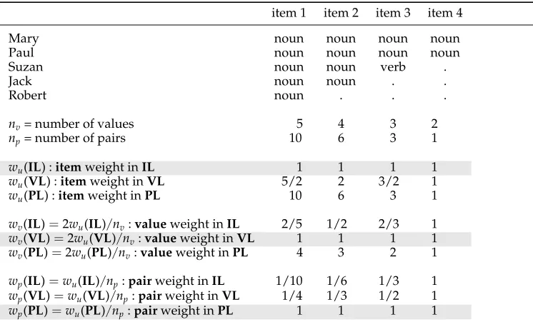
Table 1

Item, value, and pair weight comparisons in the case of five annotators with missing values (denoted by “.”)

item 1 item 2 item 3 item 4

Mary noun noun noun noun

Paul noun noun noun noun

Suzan noun noun verb .

Jack noun noun . .

Robert noun . . .

nv= number of values 5 4 3 2

np= number of pairs 10 6 3 1

wu(IL) :itemweight inIL 1 1 1 1

wu(VL) :itemweight inVL 5/2 2 3/2 1

wu(PL) :itemweight inPL 10 6 3 1

wv(IL)=2wu(IL)/nv:valueweight inIL 2/5 1/2 2/3 1

wv(VL)=2wu(VL)/nv:valueweight inVL 1 1 1 1

wv(PL)=2wu(PL)/nv:valueweight inPL 4 3 2 1

wp(IL)=wu(IL)/np:pairweight inIL 1/10 1/6 1/3 1

wp(VL)=wu(VL)/np:pairweight inVL 1/4 1/3 1/2 1

wp(PL)=wu(PL)/np:pairweight inPL 1 1 1 1

There are in the literature three very different ways to natively consider missing values in agreement coefficients, and a workaround method introduced just after:

1) itemlevel (IL). In this conception, all items are given the same weight. Conse-quently, item 4 from Table 1 is given the same weight as item 1, which is equivalent to considering that Suzan, Jack, and Robert said “noun” for item 4 although they did not say anything.

2)valuelevel (VL). This intermediate conception gives the same importance to any pairable value. Because in an item having nv values, each value can be paired with

nv−1 other values, each pair is weighted nv1−1 so that the total weight of the value

is 1.

3) pair level (PL). At the extreme opposite end of IL, this conception considers any pair of values as having the same weight as any other, whatever the item they belong to. For instance, when Mary says “noun” for item 1 (giving rise to four pairs), this weighs four times as much as when she says “noun” for item 4 (giving rise to one pair).

To better understand the differences between these three conceptions, Table 1 shows1 _{for each of them the item weight w}

u, the value weight wv, and the pair weightwp.

Key facts are: (1) wu is steady for IL by design, whereas it grows linearly with

nv for VL, and with nv(n2v−1) for PL. (2) wv reveals the opposite conceptions of IL andPL, the first decreasing and the second increasing withnv, whilewv is steady by

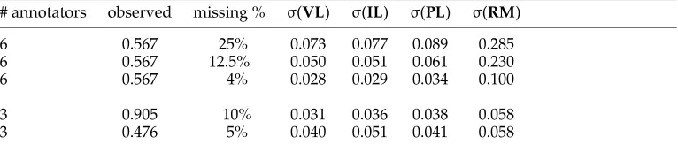
Table 2

Standard deviation of different methods when coping with missing values.

# annotators observed missing % σ(VL) σ(IL) σ(PL) σ(RM)

6 0.567 25% 0.073 0.077 0.089 0.285

6 0.567 12.5% 0.050 0.051 0.061 0.230

6 0.567 4% 0.028 0.029 0.034 0.100

3 0.905 10% 0.031 0.036 0.038 0.058

3 0.476 5% 0.040 0.051 0.041 0.058

design. (3) Because agreement measures rely on pairwise comparisons,wpdiscloses the very differences between them. There is up to a ratio of 1 to 10 between the different conceptions, which shows the importance of making the best choice among them.

Besides, a workaround method (rather than a real conception of missing values) to use measures such asκon such data, which is calledRM(for “ReMove”) hereafter, is simply to remove items that are not valued by all the annotators. In our example, items 2 to 4 would simply be discarded before computation by a standard measure.

In addition to these comparisons, to make an objective choice between these dif-ferent conceptions (and the workaround method), I have designed a specific experi-ment, reported in Table 2. Consider a set of items fully annotated byn≥3 annotators (column 1). This leads to a given observed pairwise agreement (column 2). Now con-sider the same initial set of items but with some randomly chosen missing values (with respect to the percentage shown in column 3), and apply the different conceptions of missing values to these data. The better the conceptualization of missing data, the lesser the results should diverge from complete data. The standard deviation of each conception is reported2 _{in columns 4 to 7 for 1,000,000 tests from a given set of data, each row} corresponding to certain initial data. Obviously,VLsteadily shows less deviation than all other conceptions, which makes this conception the best (known) choice under any circumstances. At the opposite end,RM(i.e., removing the whole item when value(s) is (are) missing) is the worst choice. To finish,ILandPLrank differently depending on the number of annotators and the initial observed agreement.

The αmeasure for predefined units was natively designed to cope with missing values according toVL, as explained by Krippendorff (2013, page 284): “The number of pairs of values from the values-by-units matrix [is] weighted by 1

(nu.−1) so that

each pairable value in the reliability data adds exactly one to its total count.” As a consequence, it is the measure of choice for predefined units with missing values. As a matter of fact, Krippendorff wished to have cuαbehave as a generalization ofαfor a continuum, but he failed on this point because cuα deeply relies on independent pairwise comparisons of (intersections of) units with no notion corresponding toitems: “Whilecuαignores gaps between units, it does it unlike howαignores missing values.” More precisely,cuαunfortunately relies onPL, whereasαrelies onVL. Finally, Gwet, in his attempt to adapt classical coefficients to missing values, usesIL, as we can see in equation 2.9 of Gwet (2012, page 31).

Of course,γ_cat relies on the same conception of missing values asα, namely,VL, since we have just seen that it is the best known choice. This is made possible, as we will see, thanks to its alignment process.

4. The New Coefficientγ_cat

The new coefficient being a complement toγ, it is necessary to understand the main principles of the latter, which are summed up in Section 4.1.

First of all, γ(and γ_cat) is a “chance-corrected coefficient” based on the notion of “disorder,” which assesses the level of disagreement among annotators. Hence, like other chance-corrected coefficients, it computes two values, the “observed” one, and the “expected” one, corresponding to the value we can expect under a model of chance. The observed disorder is denotedδ, and the expected disorderδ_e. Then, the corrected agreement is given by:

γ=1− δ

δ_e (1)

δ_e is computed by resampling the annotations randomly a sufficient number of times, and for each sample the disorder is computed exactly the same way as forδ, as explained in Mathet, Widl ¨ocher, and M´etivier (2015). Consequently, we will now focus only on the computation of the disorderδ, forγ,γ_cat, andγ_k.

4.1 γin a Nutshell

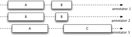
Unitizing is difficult to assess because we do not exactly know what to compare from one annotator to what from another annotator. Categorization of predefined items is much easier to assess because, by definition, items are predefined and so we know that we have to compare the first item from annotator 1 to the first item from annotator 2, and so on. But with unitizing, units from two annotators may be at the same position, or at slightly different positions, or at very different positions, as shown in Figure 3. Moreover, with some annotation material, a unit from annotator 1 may intersect with several units from annotator 2. Hence, the very first question to address is what to compare to what.

A possible method, which I will callatomization of the continuum, is to compare each atom of the continuum (for instance, at word level) from one annotator to the corresponding atom from another annotator. However, this deeply changes the nature of the data (the contiguity of units), and has severe limitations, as demonstrated in Section 3.4.1 of Mathet, Widl ¨ocher, and M´etivier (2015).

A

B

A

B

B

C

annotator 1

annotator 2

annotator 3

Figure 3

A

B

A

B

B

C

3 unitary alignments found by Gamma

3 empty units found by Gamma

annotator 1

annotator 2

annotator 3

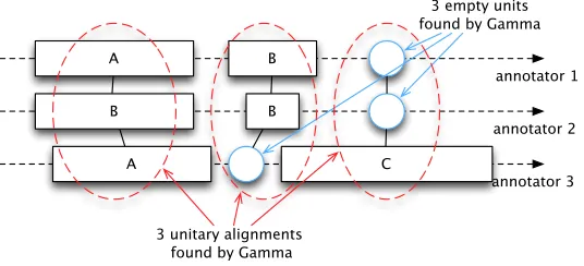
Figure 4

Unitary alignments computed byγin a holistic way.

A better method is to observe lengths of intersections between units from different annotators, as does Krippendorff with hisαsfor unitizing, but this does not overcome all the limitations of atomization (contiguity of units is not fully kept), as detailed in Section 6.1 of Mathet, Widl ¨ocher, and M´etivier (2015).

When designingγ, we considered that the best method is tocompare units to units, not atoms to atoms, nor intersecting parts of units. This ultimately consists of using an alignment of units from different annotators, as shown in Figure 4. The question is then: How do we build such an alignment? Aligning two units from two annotators consists of considering that they intended to express the same phenomenon, possibly with some discrepancies. Maybe they failed to locate the phenomenon on the exact same portion of the continuum, maybe they failed to agree on the category, maybe both, but we may consider these units to be aligned. The reason for that is that the lesser the positional discrepancy, the lesser the categorial discrepancy, the better the probability the two annotators intended to express the same thing. Of course, aligning units is a bet: Except when units completely correspond to each other both in position and category, it is not possible to affirm that they correspond to the same annotation intention. Consequently, an important idea of γ is to maximize the overall probability that all alignments are relevant.

To do so, γ uses at first the notion of “dissimilarity,” which tells how different two units are, and defines two types of dissimilarities:dpos, the positional dissimilarity, computed, for instance, as the squared relative distance between bounds of compared units, which equals zero only when positions exactly correspond, anddcat, the categorial dissimilarity, which equals zero only when categories are the same, and which may be chosen between different options like other weighted coefficients (categories considered as nominal, as values on a scale, and so on). The dissimilarity is computed for each pair of units from different annotators.

Finally,γdefines analignmentas a subset of unitary alignments that constitues a partition of the set of units (each unit appears in one and only one of the chosen unitary alignments), and the disorder of an alignment as the average disorder of its unitary alignments. Among the huge number of possible alignments, it finally retains as the best possible alignment the one that minimizes the disorder.

This is shown in Figure 4: From the data collected in Figure 3, and after a combi-natory process,γ ended by creating three unitary alignments and some empty units. In detail,γconsiders that the three annotators agree on the fact there is a first unit on the left of the continuum, but do not fully agree on its category (A, B, and A), that two annotators only consider that there is a unit in the middle of the continuum, of category B, and that only one annotator found a third unit of category C at the end of the continuum. Consequently,γhas created three empty units, one because annotator 3 missed the second unit, and two because annotators 1 and 2 missed (compared with 3) the third unit. If the second unit from annotator 3 were positioned sufficiently in the center of the continuum,γwould have chosen to generate only two unitary alignments instead of three.

A very important feature of γis that it is “unified”: It builds an alignment in the same time as it computes the agreement, because these two tasks are interlaced and based on the same assumptions. This ensures a strong consistency of the results: When the method hesitates between aligning two units or not, then the resulting computed agreements corresponding to the two choices are very close.

4.2 Introducingγ_cat

As already mentioned, we focus here only on the computation of the disorder ofγcat, which is used to calculate the observed and the expected values. To do so,γ_cat uses a four-step process, as detailed in the following sections. The main idea is to rely on an alignment of units (provided by γ) to compare the categories used by different annotators to assess the same items. In addition,γ_catuses special features to cope with theVLconception of missing values and to improve its accuracy thanks to statistical considerations.

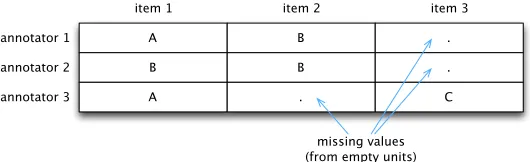
4.2.1 Obtaining an Alignment of the Units from γ.For its first step, γ_cat uses the align-ment provided byγ, which seemingly transforms a difficult unitizing problem into the simpler question of categorizing predefined items, as shown in Figure 5.3

Each unitary alignment translates into a column of a matrix, and each unit be-longing to this unitary alignment gives its category as a value in this column. Hence we obtain a very usual matrix similar to those used for predefined items. To sum up, what is usually called an “item” (and sometimes a “unit”) with predefined items corre-sponds here to a unitary alignment, and what is usually called a “value” correcorre-sponds here to the category of a unit. Of course, empty units generated byγ translate into missing values. The remaining work ofγ_catresembles what the usual α(which copes with missing values) does, but there are two important differences, as I will point out in Section 4.2.6.

3 The reason for using the alignment fromγinstead of creating an alignment that maximizes the score of

A B .

B B .

A . C

item 1 item 2 item 3

annotator 1

annotator 2

annotator 3

missing values (from empty units)

Figure 5

Resulting units/values matrix from unitary alignments.

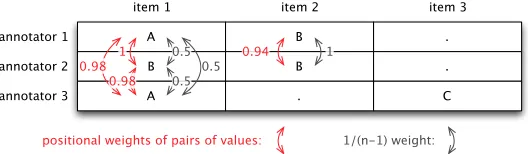
4.2.2 Value Weight: Giving the Same Importance to Each Value.As we have seen in section 3, it is important that γ_cat relies on VLconception of missing values. This is done in a simple way here, now that unitary alignments have been translated in kind of pre-defined items with possibly missing values: we just have to count the number nv of values in a column, and weight 1

nv−1 each of its pairs.

4.2.3 Confidence Weight: Enhancing the Accuracy of δ.γ_cat relies on an alignment, but as we have seen in Section 4.1, aligning is a bet, and even ifγwas designed to obtain the most likely overall alignment, it cannot ensure that a particular given pair of aligned units from two annotators really corresponds to the same intent of both of them. More precisely, some pairs are aligned with great confidence (because they correspond both in position and category) whereas others are hardly aligned (γhesitates to align them). Given this, how do we obtain the most accurate value of the (categorial) disorderδfrom our data? We could think about two opposite methods: (1) keeping only pairs of total confidence, hence relying on a trusted but very reduced set of data, or (2) considering that all pairs are of the same importance, and thus relying on fake data as much as on trusted data.

However, statistics provide a third method, through the notion of conditional ex-pectation, which takes the best from these two naive methods. To simplify the problem, let us put aside missing values, just addressed in the previous section, and consider that we have full alignments with no empty units. Under these conditions,VL,IL, and

PLconceptions are equivalent, and if we had predefined units, the categorial disorder would correspond to the average categorial dissimilarity between all pairs of units.

In the context of unitizing, let{pairi}be the set of pairs of units aligned by γ, let δ_i=dcat(pairi) be the categorial dissimilarity ofpairi, and letpibe the probability of the event calledtruePairthatpairi really corresponds to a same annotation intent for both annotators.

LetDbe the random variable defined as the function of dissimilarity between pairs of units from different annotators. The categorial disorder δ we want to estimate is the average value taken by D for true pairs only, which formally corresponds to the conditional expectation ofDgiven the eventtruePair, and is given by Equation (2):

δ=E(D|truePair)=P1 i(pi)

·X

i

(pi·δi) (2)

For our purpose, I built the probabilitypion positional ground only, because taking categories into account would bias the results: Agreements (on categories) would be more weighted than disagreements, which would lead to a lowered overall disorder value. Consequently, the probability pi is designed so that it equals 1 for two units positioned at the exact same location (dpos=0), and so that it reaches 0 whenγbegins to prefer not aligning them because of too much difference in positions (that is to say, whendposreaches 1): forpairi=(uj,uk),pi=max(0, 1−dpos(uj,uk)).

I call this value “pairing confidence,” and it is a second weight that will be taken into account in the global computation. Experiments with the Corpus Shuffling Tool (introduced later) have confirmed the benefits of using the notion of confidence weight, which provides an agreement value of 0 with random annotations (which is correct), whereas when not using it, agreement may be slightly below 0 (which is not desirable).

4.2.4 Total Weight of a Pair of Units.Figure 6 illustrates both the value weight and the pairing confidence weight for each pair of units (i.e., for each pair of values in the table) for the data coming from Figure 3. The total weight for a given pair of units is the product of its value weight and its confidence weight. For instance, the total weight for the pair annotator 1 with annotator 3 of item 1 is 0.5 (because there are three values for this item) multiplied by 0.98 (because of the slight positional discrepancy), which is 0.49.

4.2.5 The Algorithm to Compute the Disorder ofγ_cat.We can now formally define all the steps of the computation of the disorder ofγcat. The detailed procedure is provided in Algorithm 1.

First of all, let us recap the γ terminology: ˆais the best possible alignment com-puted byγ—that is which minimizes the total disorder of its unitary alignments. The unitary alignments are denoted ˘a, and each of them contains one or zero unit from each annotator, denotedu1tounv.

The first step, at line 1, is to obtain ˆaexactly asγdoes.

Then, a loop, from line 4 to line 14, computes the contribution of each unitary align-ment to the total disorder. To do so, it considers the number of true units (i.e., not empty ones) contained in the unitary alignment, and then computes the 1

nv−1 weight shared by

all pairs of units. Then, it uses a sub-loop to enumerate each possible pair of units of the unitary alignment. For each of them, it computes its (categorial) dissimilarity, its own confidence weight, and thus obtains its resulting weight (product of the shared weight and the confidence weight) and its disorder contribution.

At the end of the main loop, we obtain the total disorder contribution and the total weight, hence the total disorder.

A B .

B B .

A . C

item 1 item 2 item 3

annotator 1

annotator 2

annotator 3

0.94 0.98 1

0.98

positional weights of pairs of values: 0.5

0.5

1 0.5

1/(n-1) weight:

Figure 6

Algorithm 1Computation of the total disorder

1: Compute an alignment ˆaby using the normalγdissimilaritydcombi=dpos+dcat

2: disordertotal←0

3: weighttotal←0

4: for all˘a∈aˆdo

5: nv←number of real units in ˘a(exludingu∅)

6: weightbase ← nv1−1 7: for all(ui,uj)∈a˘do

8: weightconfidence←max(0, 1−dpos(ui,uj))

9: weight←weightbase×weightconfidence

10: dissimilarity←dcat(ui,uj)

11: disordertotal←disordertotal+dissimilarity×weight

12: weighttotal←weighttotal+weight

13: end for

14: end for

15: return disordertotal/weighttotal

4.2.6 Discussion: Why We Should Not Use a Naive Two-Step Method.Of course, to build such a coefficient, one might think to use a naive method that consists, first, in gen-erating an alignment thanks to γ, and second, in applying theα measure (for pre-defined units) to the resulting matrix (as the one shown in Figure 5). However, doing so, we would miss two important points: (1) Obviously, we would not benefit from the statistical enhancement provided by the confidence weight; (2) A more hidden problem is that the expected value computed byαwould be biased. Indeed, when units are of different lengths, mixing tabulated values coming from an alignment is not the same as resampling unitized units and then aligning them. For instance, in the example of Figure 7 (left: unitizing, right: resulting matrix), the naive method would provide an expected valueδ_e=0.5 (what we obtain in average from 50% of A and 50% of B), whereas γ_cat would provide δ_e=1, since A and B would never be aligned because of too much difference in lengths, and so only A-A and B-B pairs would occur when resampling unitized units.

4.3 The In-depth Coefficientγ_kthat Focuses on Each Category

γ_kworks the same way asγ_catdoes, except for the fact that it focuses on each particular category, and so provides not just one agreement value, but as many agreement values as the number of categories. For instance, if there are three categories A, B, and C in the annotations,γ_kwill provide three agreements, namely,γ_k(A),γ_k(B), andγ_k(C). I have chosen the letter “k” by reference tokαfrom Krippendorff, which shares the same goal.

A

A

B

B

annotator 1

annotator 2

A B

A B

item 1 item 2

Figure 7

By focusing on a given category, for instance A, this measure will only look at what a unit of type A is combined with: in our example, A with A, A with B, A with C, but not B with C. Hence, it isγ_cat reduced to a subset of pairs of units, only the ones that contain at least one unit of type A.

It is very simple to design γ_k from γcat: We just have to add one condition in Algorithm 1 so that we keep only relevant pairs of units. More precisely, we add the condition (cat(ui)=k)∨(cat(uj)=k) to line 7 to focus on pairs that concern (at least) one unit of categorykonly:

7: for all(ui,uj)∈˘a|(cat(ui)=k∨cat(uj)=k)do

Of course, the computation is done as many times as the number of categories, because several agreement values are provided:γ_kis in fact a set of measures.

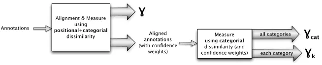
4.4 Overview and Dependencies of the Gamma Family

Now thatγ_cat and γ_k have been introduced on the basis of γ, let us recap the links between the three measures, as illustrated in Figure 8.

From the multi-annotator annotations, the unified and holist method is used to computeγ and to generate an alignment at the same time. This process relies on an overall dissimilarity that combines positional and categorial dissimilarities. Then, from the alignment and the confidence weights which have been computed byγ, and using only the categorial dissimilarity from the previous step,γ_catandγ_kare computed.

5. Benchmarking

The benchmarking is organized as follows: First, I confirm thatγ_catbehaves the correct way when dealing with missing values in Section 5.1. Second, I make an in-depth com-parison betweenγ_catandcuα, the first and only other measure devoted to categorization of a continuum, in Section 5.2. Third, from Section 5.3 to Section 5.8, I propose six experiments using the Corpus Shuffling Tool from Mathet et al. (2012) to observe how γ_catresponds to different kinds of discrepancies. This tool and the associated kinds of experiments are fully described in Mathet, Widl ¨ocher, and M´etivier (2015, page 467), the paper in whichγwas benchmarked this way.

Alignment & Measure using positional+categorial

dissimilarity

Ɣ

Aligned annotations (with confidence

weights) Annotations

Measure using categorial dissimilarity (and confidence weights)

Ɣ_cat Ɣ_k each category all categories

Figure 8

5.1 Start Point: Predefined Items with Missing Values

γ_cat being a coefficient for categorization of a continuum, I designed it to be a gen-eralization to a continuum of what I consider to be the best available measure for categorization of predefined items with missing values, namely,α.

To do so, I have done experiments with predefined data translated into a continuum in a simple manner: The first item occupies position 0 to position 1 of the continuum, the second one position 1 to position 2, and so forth. Each time,γ_catobtains exactly the same observed value as α, and an approximate value of the expected value of αfor sampling reasons, as explained in Mathet, Widl ¨ocher, and M´etivier (2015). For instance, with the example from Krippendorff (2011, page 9) as shown in the screenshot of Figure 9, with 4 annotators, 12 items, and 7 missing units,α=0.743 and 0.74< γ_cat< 0.76, with the same observed disagreement 0.2. Hence,γ_catproves to be a good approx-imate generalization ofαto unitizing.

On the other hand, because it relies onPL, as discussed in Section 3,cuαprovides an agreement value of 0.715, and confirms that it fails to generalizeα, being here more conservative, but possibly less conservative with other data. In particular, its observed disagreement is 0.218 instead of 0.2 forαandγcat, which confirms a structural difference of how to take missing values into account.

5.2 A Detailed Illustration of the Differences Betweenγ_catandcuα

It is illuminating to see some important differences between the conceptions of γ_cat andcuα, with the data from Figure 3.

cuα computes all intersections between units from different annotators, as shown in Figure 10, with a total intersection length of 31. Then, the contribution of a pair of categories in the computation of the coefficient is given by its relative total size. For instance, for B with B pairs, the total intersection length is 3, hence a contribution of 3/31=9.7%. In a radically different way, γ_cat combines two weights, one for taking into account missing values, the other for pairing confidence, as shown in Figure 6.

Figure 9

A predefined unit corpus translated to a continuum.

A-A A-B

B-A

B-B

B-C B-C

Figure 10

Table 3

Comparison of the relative contribution, in percent, of each category pair forγ_catandcuα.

A with A B with B A with B B with C A with C

γcat 20.2 38.8 40.9 -

-cuα 25.8 9.7 54.8 9.7

-For instance, for B with B, we get a contribution of 0.94×1=0.94, out of a total weight of 2.42 (not detailed here), hence a contribution of 38.8%.

The results of all pairs of categories are given in Table 3. We can see very deep differences between the two conceptions. It is particularly striking that forcuα, there is as much agreement thanks to B with B as there is disagreement because of B with C, both at 9.7%, whereas forγ_cat, there is 38.8% agreement from B with B, and no disagreement from B with C. The reason is that the two units of type B that intersect are small, hence their low contribution tocuα. Since these two units are not being aligned with a third one, theVLcoefficient 1

nv−1 =1 of this pair is twice as much as the

1 nv−1 =

1

2 coefficient of the other pairs from the three aligned units.

In addition, for the same reasons, B with B is about twice as much as A with A for γ_cat, and it is the contrary forcuα.

Finally, for all these reasons,γ_catandcuαshow very different agreement values on this example of, respectively, 0.36 forγ_catand 0.08 (almost no agreement at all) forcuα. Moreover, it is particularly striking thatk(B)α=−0.149 (worse than by chance), whereas γ_k(B)=0.484, which makes a huge difference of 0.633.

5.3 Categorial Stability to Positional Discrepancies

A very important feature of a categorial measure for unitizing is its stability to positional discrepancies: The very aim of such a measure is not to respond at all to discrepancies that are not categorial. It is the first requirement introduced in Section 2.

The shuffling tool was set with a pure positional shuffling: Units from the reference are moved (the higher the magnitude, the more the shifts) but the categories are pre-served. It is important to understand that a so-called pure positional shuffling ends up having consequences on categories: If we move two very distant units (from two anno-tators) very much, their new positions may superimpose. Hence, in the range of high magnitudes (from 0.75 to 1), many pairs of units are concerned by this phenomenon and it is normal that this shuffling ends up affecting categorial measures.

Three measures have been submitted:γcat,γ, andcuα, as shown in Figure 11. γ_catclearly shows the best behavior. It remains at 1 up to magnitude 0.55, and is still above 0.9 at high magnitude 0.8.

On the contrary, cuα starts to decrease at very low magnitudes, almost linearly, and is already at 0.5 at magnitude 0.8. This is the consequence of what is shown in Figure 15 later in this article: As soon as two units start to overlap,cuαconsiders the resulting intersection as an intent of the annotators to categorize the same object (a portion of the continuum), whereasγ_cat(and alsoγ) only compares aligned units, not sets of intersections.

Figure 11

Categorial stability to positional discrepancies.

theγvalue corresponds to positional (and false negatives/positives, see next section) discrepancies.

5.4 Categorial Stability to False Negatives/Positives

For this test, the shuffling tool was set with false negatives only, because false positives may bring some overlapping units, but for symmetry reasons (a false positive from one annotator corresponds to a false negative from another), there is no real difference with false positives for the measures.

Bothγ_cat andcuαare at 1, which is desirable and easy to understand (some units are removed, but the remaining ones are unchanged), andγ is about the same as for positional discrepancies (no figure is needed here). This confirms the complementarity ofγandγcat.

5.5 Categorial Discrepancies

In order to be accurate and progressive in the benchmarking of measures, I address here the question of categorial discrepancies of units of homogeneous sizes. Indeed, we will see in a further section that size may affectcuα.

Figure 12 shows thatγ_cat andcuαare about the same, decreasing quite regularly from 1 to 0, as expected. On the contrary,γgoes from 1 to 0.35, because positions are still correct. The two gammas are once again complementary: Aγvalue higher than the γ_catvalue means that the disagreement is mainly due to categorization.

5.6 Categorial Plus Positional Discrepancies

To refine the results, we can combine categorial and positional discrepancies in the shuffling tool, as reported in Figure 13.

Figure 12

Categorial discrepancies.

Figure 13

Categorial plus positional discrepancies.

A second point is thatcuαdoes not show the same stability, and is lowered by the positional discrepancies. In particular, from magnitudes 0.1 to 0.6, there is a difference of up to 0.06, which is not negligible. These differences, though, are much lower than with positional discrepancies (cf. Figure 11) mainly because, the values being much lower, and the differences being proportional to the values, they are also much lower.

Third, γ is now clearly lower than γ_cat because it depends on the two kinds of discrepancies used here, instead of one forγ_cat.

5.7 Units of Various Sizes

γ_catwas designed not to be dependent on size of units, contrary tocuα. To confirm this conceptual difference with the shuffling tool, I have set two experiments in which there are four categories, and where annotators make more and more confusions within the three categories A, B, and C, but keep making no mistake for category D. In the first experiment, all units are of size 5. In the second experiment, units of categories A, B, and C still are of size 5, but those of category D are of size 20.

Figure 14

Length variations on categorial discrepancies.

the second one, it is much higher, being twice as much as γ_cat at magnitude 1 (0.54 versus 0.27).

5.8 Benchmarkingγ_k

To finish, for this experiment dedicated to testγ_k, I have once again used four categories A, B, C, and D, with no mistake for category D. Of course,γ_k(D)remains at 1, andγ_k(A), γ_k(B), andγ_k(C)decrease from 1 to about 0.1 (Figure 15). We may wonder why they do not reach 0, but this is normal and the reason is that there is no confusion between each for these categories and category D, contrary to what happens for the expected value which has this additional discrepancy.

γ_cat reaches about 0.33 at magnitude 1, but this overall result would not reveal by itself the fact that only three categories out of four are confusing for the annotators. Hence the usefulness of the additional coeffcientγ_kis demonstrated.

6. Software

The full implementation of theγ family (γ,γcat, andγk) is provided as free software on thehttp://gamma.greyc.frWeb site. It is a standalone application written in Java,

Figure 15

which runs on any platform, and successfully tested on Mac OS X, Windows, and Linux. It is also available as a Web service for those who do not want to install it. It is compatible with annotations created with the Glozz Annotation Platform (Widl ¨ocher and Mathet 2012), and with annotations generated by the Corpus Shuffling Tool (Mathet et al. 2012). Because these formats rely on simple and public comma-separated value specifications, it is easy to translate other formats to these.

The application comes with a graphical user interface, as shown in the screenshot of Figure 16. The window is divided into three panels, respectively, from top to bottom, the settings, the results, and the annotations. In the Settings panel, one can choose the measure(s) to apply, eitherγ, or bothγ_cat and γ_k. One may also set the desired precision to compute the expected value, because, as explained in Mathet, Widl ¨ocher, and M´etivier (2015, page 460), the latter is computed by sampling. In the Results panel, all the results are detailed: the agreement, observed and expected values, and also the number of unitary alignments found. In the example, the user chose 2% of precision for the expected value, henceγ_catis known to be between 0.34 and 0.37 with a 95% degree of confidence. Also, the values ofγ_kare provided for the three categories, andγ_k(C)is not available (NA) because there is no pair of units containing at least one unit of category C. When the user loads a new file of annotations, or when she changes a setting, the computation is automatically relaunched, so that the results always correspond to what is shown in the interface.

In our example,γ_cat is quite low at 0.36, because of confusions between categories A and B, since category C does not contribute to the result as we have just seen. To go deeper into details,γ_kshows us that this low agreement is due more to category A (γ_k(A)=0.335) than to category B (γ_k(B)=0.494). Moreover,γ=0.29 (not visible in the screenshot because one has to click on “Gamma” to make it appear) is quite close toγ_cat, which tells us that the annotators have to improve both unitizing and categorization.

Figure 16

7. Conclusions

In computational linguistics, when annotation efforts are relative to a continuum rather than to predefined items, researchers are not typically provided with methods and tools to assess the agreement among several annotators. Recently, γ proposed an overall solution that takes into account all kinds of discrepancies (categories, positions, false positives, and false negatives) in order to assess whether the multi-annotations are reliable or not. However, when the agreement is not as good as is wished, the researchers would like to have more details about the discrepancies, in order to better understand the difficulties and thus to enhance the annotation model or the annotation manual. In particular, is a given overall low agreement due to poor specification of categories? Or even of some particular categories?

The aim of this work is to provide such complements to γ, with two additional coefficientsγ_catandγ_k, which focus on the categorization part of the agreement, with the expectation that they also fulfill three important requirements for computational linguistics: (1) Positional discrepancies should not impact categorial agreement; (2) Length of units should not be taken into account; (3) Missing values should be tackled appropriately.

Finally, this research addresses a neglected question: How do we assess the reliabil-ity of annotators to categorize a continuum, whatever their discrepancies in positioning units. Only Krippendorff proposes solutions, with his coefficientscuαandkα, but with different assumptions from the ones we posit for computational linguistics needs. In particular, relying on intersections rather than on an alignment, these coefficients mostly compare quantities of occupied space rather than genuine units.

γ_catwas designed not only as a complement toγ, but also with the same conception of how to handle unitizing, and with a common alignment process. Relying on an alignment, it compares genuine units and so ensures requirements (1) and (2).

Because the aim ofγ_catis somehow to extend what agreement measures do for pre-defined items to the case of unitizing a continuum, it was important thatγ_catperform as well as the best specialized measures. Moreover, the context of free unitizing leads to a great number of so-called missing values (when some annotators put units where others do not), which led me to frontally study this other neglected question for requirement (3): How should a measure natively handle missing values? I made a thorough analysis of the question and formulated a clear answer: The best solution is to do as the classic αmeasures does (and as cuαunfortunately fails to do). This is also a result that goes beyond the scope of this article focused on unitizing.γ_catmanages to do (almost) exactly the same asαwhen restrained to the simpler case of predefined units, which constitutes a strong basis.

Finally, γ_cat fulfills all the requirements expressed for computational linguistics. Experiments with the shuffling tool confirm all these capabilities, as well as the fact that the three coefficientsγ,γ_cat, andγ_kare complementary.

These coefficients are already implemented, ready to use, and freely available.

Acknowledgments

I wish to thank three anonymous reviewers for their very helpful comments and suggestions. The author also thanks Klaus Krippendorff for discussions and

collaborations over the years, which

References

Artstein, Ron and Massimo Poesio. 2008. Inter-coder agreement for computational linguistics.Computational Linguistics, 34(4):555–596.

Cohen, Jacob. 1960. A coefficient of

agreement for nominal scales.Educational and Psychological Measurement, 20(1):37–46. Cohen, Jacob. 1968. Weighted kappa:

Nominal scale agreement with provision for scaled disagreement or partial credit.

Psychological Bulletin, 70(4):213–220. Fleiss, Joseph L. 1971. Measuring nominal

scale agreement among many raters.

Psychological Bulletin, 76, 5:378–382. Fretwurst, Benjamin. 2015. Reliability and

accuracy with lotus. InProceedings of the 65th ICA Annual Conference, San Juan. Gwet, Kilem Li. 2012.Handbook of Inter-rater

Reliability, third ed. Advanced Analytics, LLC.

Krippendorff, Klaus. 1980.Content Analysis: An Introduction to Its Methodology, chapter 12. Sage, Beverly Hills, CA. Krippendorff, Klaus. 1995. On the reliability

of unitizing contiguous data.Sociological Methodology, (25):47–76.

Krippendorff, Klaus. 2004.Content Analysis: An Introduction to Its Methodology, 2nd edition, chapter 11. Sage, Thousand Oaks, CA.

Krippendorff, Klaus. 2011. Agreement and information in the reliability of coding.

Communication Methods and Measures, 5(2):93–112.

Krippendorff, Klaus. 2013.Content Analysis: An Introduction to Its Methodology, 3rd edition, chapter 11. Sage: Thousand Oaks, CA.

Krippendorff, Klaus, Yann Mathet, St´ephane Bouvry, and Antoine Widl ¨ocher. 2016. On the reliability of unitizing textual continua: Further developments.Quality and Quantity, 50(6):2347–2364.

Mathet, Yann, Antoine Widl ¨ocher, Kar¨en Fort, Claire Francois, Olivier Galibert, Cyril Grouin, Juliette Kahn, Sophie Rosset, and Pierre Zweigenbaum. 2012. Manual corpus annotation: Giving meaning to the evaluation metrics. InCOLING 2012, pages 809–818, Mumbai.

Mathet, Yann, Antoine Widl ¨ocher, and Jean-Philippe M´etivier. 2015. The unified and holistic method gamma (γ) for inter-annotator agreement measure and alignment.Computational Linguistics, 41(3):437–479.

Scott, William. 1955. Reliability of content analysis: The case of nominal scale coding.Public Opinion Quarterly, 19(3):321–325.