Munich Personal RePEc Archive
Improving Markov switching models
using realized variance
Liu, Jia and Maheu, John M
McMaster University
1 September 2015
Online at
https://mpra.ub.uni-muenchen.de/71120/
Improving Markov Switching Models using Realized
Variance
∗
Jia Liu
†John M. Maheu
‡August 2015
Abstract
This paper proposes a class of models that jointly model returns and ex-post variance measures under a Markov switching framework. Both univariate and multivariate re-turn versions of the model are introduced. Bayesian estimation can be conducted under a fixed dimension state space or an infinite one. The proposed models can be seen as nonlinear common factor models subject to Markov switching and are able to exploit the information content in both returns and ex-post volatility measures. Applications to U.S. equity returns and foreign exchange rates compare the proposed models to existing alternatives. The empirical results show that the joint models improve den-sity forecasts for returns and point predictions of return variance. The joint Markov switching models can increase the precision of parameter estimates and sharpen the inference of the latent state variable.
Keywords: infinite hidden Markov model, realized covariance, density forecast, MCMC
∗We thank Qiao Yang for comments. Maheu is grateful to the SSHRC for financial support. †DeGroote School of Business, McMaster University, Canada, [email protected]
1
Introduction
This paper proposes a new way of jointly modelling return and ex-post volatility measures under a Markov switching framework. Both parametric and nonparametric versions of the proposed joint models are introduced in both univariate and multivariate settings. The proposed models exploit the information content in both return and ex-post volatility series. Compared to existing models, the proposed models improve density forecasts of returns and point predictions of realized variance.
Since the pioneering work by Hamilton (1989) the Markov switching model has became one of the standard econometric tools in studying various financial and economic data se-ries. The basic model postulates a discrete latent variable governed by a first-order Markov chain that directs an observable data series. This modelling approach has been fruitfully applied in many applications. For instance, Markov switching models have been used to iden-tify bull and bear markets in aggregate stock returns (Maheu & McCurdy 2000, Lunde & Timmermann 2004, Maheu et al. 2012), to capture the risk and return relationship (Pastor & Stambaugh 2001, Kim et al. 2004), portfolio choice (Guidolin & Timmermann 2008), interest rates (Ang & Bekaert 2002, Guidolin & Timmermann 2009) and foreign exchange rates (Engel & Hamilton 1990, Dueker & Neely 2007). Recent work has extended the Markov switching model to an infinite dimension. The infinite hidden Markov model (IHMM), which is a Bayesian nonparametric model, allows for a very flexible conditional distribution that can change over time. Applications of IHMM include Jochmann (2015), Dufays (2012), Song (2014), Carpantier & Dufays (2014) and Maheu & Yang (2015).
Realized variance (RV), constructed from intraperiod returns, is an accurate measure of ex-post volatility. Andersen et al. (2001) and Barndorff-Nielsen & Shephard (2002) formal-ized the idea of using higher frequency data to measure the volatility of lower frequency data and show RV is a consistent estimate of quadratic variation under ideal conditions. Barndorff-Nielsen & Shephard (2004b) generalized the idea of RV and introduced a set of variance estimators called realized power variations (RPV). Furthermore, RV has been ex-tended to realized covariance (RCOV), which is an ex-post nonparametric measure of the covariance of multivariate returns, by Barndorff-Nielsen & Shephard (2004a). A good survey of RV and related volatility proxies is Andersen & Benzoni (2009).
This paper is not the first to exploit the information content of RV to improve model estimation. Takahashi et al. (2009) propose a stochastic volatility model in which unobserved log-volatility affect both RV and the variance of returns. They find improved fixed parameter and latent volatility estimates but do not investigate forecast performance. Similarly, we develop joint Markov switching models in which the latent state variable enters both returns and RV. Finite as well as infinite Markov switching models are considered. Our focus is on the gains to forecasts this approach can provide. In addition, there is no reason to confine attention to RV, and therefore we investigate the use of other volatility measure and in the multivariate setting realized covariance.
Four versions of the univariate return models are proposed. We consider RV, log(RV), realized absolute variation (RAV), or log(RAV) as ex-post volatility measures coupled with returns to construct joint models. We then extend the MS-RV specification to its multivariate version with RCOV.
number of states needed to fit the data. Using Bayesian nonparametric techniques, we extend the finite state joint MS models to nonparametric versions. These models allow the conditional distribution to change more flexibly and accommodate any nonparametric relationship between returns and ex post volatility.
The proposed joint MS and joint IHMM models are compared to existing models in empirical applications to equity and foreign exchange data. The univariate return models are applied to monthly U.S. stock market returns and monthly foreign exchange exchange rates. Based on the log-predictive Bayes factors, the proposed joint models strongly dominate the models that only use returns. Moreover, we find the gains from joint modelling are particularly large during high volatility episodes. The empirical results also show that the joint models reduce the error in predicting realized variance. With the help of additional information offered by RV, RAV and RCOV, the parameters have shorter posterior density intervals and the inference on the unobservable state variables are potentially improved.
This paper is organized as follows. In section 2, we show how to incorporate ex post measures of volatility into Markov switching models. The joint MS models are extended to the nonparametric versions in section 3. Benchmark models used for comparison are found in Section 4. Section 5 illustrates the Bayesian estimation steps and model comparison. Uni-variate return applications are in Section 6 while multiUni-variate applications are in Section 7. The next section concludes followed by an appendix that gives detailed steps of posterior simulation.
2
Joint Markov Switching Models
In this section, we will focus on simple specifications of the conditional mean but dynamic models with lags of the dependent variables could be used. We will first discuss the four versions of univariate return joint models, then introduce the multivariate version.
Higher frequency data is used to construct ex post volatility measures. Let rt,i denotes
the ith intraperiod continuously compounded return in period t, i = 1, . . . , n
t, where nt is
the number of intraperiod returns. Then the return and realized variance from t−1 to t is
rt = nt X
i=1
rt,i, (1)
RVt = nt X
i=1
rt,i2 . (2)
Andersen et al. (2001) and Barndorff-Nielsen & Shephard (2002) formalized the idea of using higher frequency data to measure the volatility of rt. They show that RVt is a consistent
estimate of quadratic variation under ideal conditions.1 Similarly, for multivariate returns
Rt,i is theithintraperiodd×1 return vector at timetand the timetreturn isRt =Pnti=1Rt,i. RCOVt denotes the associated realized covariance (RCOV) matrix which is computed as
1
follows,
RCOVt= nt X
i=1
Rt,iR
′
t,i. (3)
For notation, let r1:t = {r1, . . . , rt}, RV1:t = {RV1, . . . , RVt}, y1:t = {y1, . . . , yt} where yt={rt, RVt}. We further define R1:T ={R1, . . . , RT}, RCOV1:T ={RCOV1, . . . , RCOVT}
and Y1:t ={Y1, . . . , Yt} where Yt={Rt, RCOVt}.
2.1
MS-RV Model
We first use RV as the proxy for ex-post volatility to build a joint MS-RV model. The proposed K-state MS-RV model is given as follows.
rt
st ∼ N(µst, σ2st), (4)
RVt
st ∼ IG(ν+ 1, νσst2), (5)
Pi,j = p(st+1 =j|st =i), (6)
wherest∈ {1, . . . , K}. Conditional on statest,RVt is assumed to follow an inverse Gamma
distribution2 IG(ν + 1, νσ2
st), where ν + 1 is the shape parameter and νσst2 is the scale
parameter.
The basic assumption of this model is that RVt is subject to the same regime changes
as rt and share the same parameter σst2.3 Note, that RVt and the other volatility measures
used in this paper, are assumed to be a noisy measure of the state dependent variance σst2. Conditional on the latent state, the mean and variance of RVt are
E(RVt|st) =
νσ2st
(ν+ 1)−1 =σ
2
st, (7)
Var(RVt|st) =
(σ2
st)2
(ν−1). (8)
Therefore RVt is centered around σst2, but in general, not equal to it. The variance of the
distribution of RVt is positively correlated with the realized variance itself. During high
volatility periods, the movements of realized variances are more volatile. Both the return process and realized variance process are governed by a same underlying Markov chain with transition matrix P.
Since σ2st influences both the return process andRVt process, the model can be seen as a
nonlinear factor model. Exploiting the information content of RVt forσst2 may lead to more
precise estimates of model parameters, state variables and forecasts.
2Ifx
∼IG(α, β),α >0,β >0 then it has density function:
g(xα, β) = β α
Γ(α)x
−α−1
exp
−βx
The mean ofxisE(x) = αβ−1 forα >1.
3Formally, the high frequency data generating process is assumed to be r
t,i = µst/nt+ (σst/
√n
t)zt,i, withzt,i∼NID(0,1). ThenE[Pn
t
i=1r 2
t,i
st] = (µst/nt)
2+σ2
st ≈σ
2
st when the term (µst/nt)
2is small due to
n2
2.2
MS-logRV Model
Another possibility is to model the logarithm of RV as normally distributed. The MS-logRV model is shown as follows,
rt
st ∼ N (µst,exp(ζst)), (9)
log(RVt)
st ∼ N
ζst −
1 2δ
2
st, δ2st
, (10)
Pi,j = p(st+1 =j|st =i), (11)
where st ∈ {1, . . . , K}. In this model there are three state-dependent parameters: µst, ζst
and δ2
st, which enable both the mean and variance of returns and log(RVt) to be
state-dependent. ζst − 12δ2st is the mean of log(RVt) and exp(ζst) is the variance of returns. Since RVt is log-normal, E[RVt|st] = exp(ζst) which is assumed to be the variance of returns.
2.3
MS-RAV Model
Now we consider using realized absolute variation (RAV), instead of RV in the joint MS model. Calculated using the absolute values of intraperiod returns, RAV is robust to jumps and may be less sensitive to outliers (Barndorff-Nielsen & Shephard 2004b). RAVt is
com-puted using intraperiod returns as
RAVt = r π 2 r 1 nt nt X i=1
|rt,i|, (12)
where rt,i denotes the ith intraperiod log-return in period t, i = 1, . . . , nt. It can be shown
that RAVt provides estimate of the standard deviation of rt.4
Consistent with the inverse gamma distribution to model the variance or its proxy, we as-sume RAV follows a square-root inverse gamma distribution (sqrt-IG). The density function of sqrt-IG(α, β) is given by
f(x) = 2β
α
Γ(α)x
−2α−1
exp
−xβ2
, x > 0, (13)
and the first and second moments of sqrt-IG(α, β) are given as follows
E[x] =pβ· Γ(α−
1 2)
Γ(α) and E[x
2] = β
α−1. (14)
These results can be found in Zellner (1971).
We define the joint MS model of return and RAV as,
rt
st ∼ N(µst, σst2), (15)
RAVt
st ∼ sqrt-IG ν, σst2
Γ(ν) Γ(ν− 12)
2!
, (16)
Pi,j = p(st+1 =j|st=i), (17)
4As before, if r
t,i = µst/nt+ (σst/
√n
t)zt,i, with zt,i ∼ N ID(0,1) and µst/nt is small, then we have
E p π 2 q 1 nt nt P
i=1|
rt,i|
st
where st ∈ {1, . . . , K}. As in the MS-RV model, the mean and variance of both rt and RAVtare state-dependent. In each state, the return follows a normal distribution with mean µst and variance σst2. The mean and variance of RAVt conditional on state st are given as
follows.
E(RAVt
st) = σst, (18)
Var(RAVt st) =
σ2st ν−1
Γ(ν) Γ(ν− 12)
2
−σst2. (19)
2.4
MS-logRAV Model
Similar to the MS-logRV model discussed in Section 2.2, the logarithm of RAV can be modelled as opposed to RAV. The MS-logRAV specification is
rt
st ∼ N (µst,exp(2ζst)), (20)
log(RAVt)
st ∼ N
ζst −
1 2δ
2
st, δst2
, (21)
Pi,j = p(st+1 =j|st=i), (22)
where st ∈ {1, . . . , K}. The model is close to the MS-logRV parametrization, but now ζst−12δst2 is the mean of log(RAVt) and exp(2ζst) is the state-dependent variance of returns.
SinceRAVt is log-normal,E(RAVt|st) = exp(ζst) which is the standard deviation of returns.
2.5
MS-RCOV Model
The univariate return models can be extended to the multivariate setting by including real-ized covariance matrices. The multivariate MS-RCOV model we consider is
Rt
st ∼ N (Mst,Σst), (23)
RCOVt
st ∼ IW (Σst(ν−d−1), ν), ν > d+ 1, (24) Pi,j = p(st+1 =j|st=i). (25)
where st ∈ {1, . . . , K}. Mst is a d×1 state-dependent mean vector and Σst is the d×d
covariance matrix. RCOVtis assumed to follow an inverse Wishart distribution5 IW(Σst(ν− d−1), ν), where Σst(ν−d−1) is the scale matrix and ν is the degree of freedom.
Σst is the covariance of returns as well as the mean of RCOVt since
E[RCOVt st] =
1
ν−d−1Σst(ν−d−1) = Σst, (26) assuming ν > d+ 1. The parameter ν controls the variation of the inverse Wishart distri-bution and the smallerν is, the larger spread the distribution has. BothRtand RCOVt are
governed by the same Markov chain with transition matrix P.
5If ad-dimension positive definite matrixX
∼IW(Ψ, ν), its density is
g(XΨ, ν) = |Ψ|
ν 2
2ν d2 Γ
d(ν2)
|X|−ν+d+12 exp
−12tr ΨX−1
3
Joint Infinite Hidden Markov Model
3.1
Dirichlet Process and Hierarchical Dirichlet Process
All of the Markov switching models we have discussed require the econometrician to set the number of states. An alternative is to incorporate the state dimension into estimation. The Bayesian nonparametric version of the Markov switching model is the infinite hidden Markov model, which can be seen as a Markov switching model with infinitely many states. Given a finite dataset, the model selects a finite number of states for the system. Since the number of states is no longer a fixed value, the Dirichlet process, an infinite dimensional version of Dirichlet distribution, is used as a prior for the transition probabilities.
The Dirichlet process DP(α, H), was formally introduced by Ferguson (1973) and is a distribution of distributions. A draw from a DP(α, H) is a distribution and is almost surely discrete and centered around the base distributionH. α >0 is the concentration parameter that governs how close the draw is toH.
We follow Teh et al. (2006) and build an infinite hidden Markov model (IHMM) using a hierarchical Dirichlet process (HDP). This consists of two linked Dirichlet processes. A single draw of a distribution is taken from the top level Dirichlet processes with base measureHand precision parameter η. Subsequent to this, each row of the transition matrix is distributed according to a Dirichlet processes with base measure taken from the top level draw. This ensures that each row of the transition matrix governs the moves among a common set of model parameters. In addition, each row of the transition matrix is centered around the top level draw but any particular draw will differ. If Γ denotes the top level draw andPj the jth
row of the transition matrix P then the previous discussion can be summarized as
Γη ∼ DP(η, H), (27)
Pj
α,Γ iid∼ DP(α,Γ), j = 1,2, .... (28)
Combining the HDP with the state indicator st and the data density, forms the infinite
hidden Markov model,
Γη ∼ DP(η, H), (29)
Pj
α,Γ iid∼ DP(α,Γ), j = 1,2, ..., (30)
st
st−1, P ∼ Pst−1, (31)
θj iid
∼ H, j = 1,2, ..., (32)
yt
st, θ ∼ F(yt
θst), (33)
whereθ ={θ1, θ2, ...}andF(·|·) is the data distribution. The two concentration parametersη
andαcontrol the number of active states in the model. Larger values favour more states while small values promote a parsimonious state space. Rather than set these hyperparameters they can be treated as parameters and estimated from the data. In this case, the hierarchical prior for η and α are
η ∼ G(aη, bη), (34)
where G(a, b) stands for the gamma distribution6with shape parameteraand rate parameter
b. The models can be estimated with MCMC methods. We discuss the specific details below for each model.
3.2
IHMM with RV and RAV
RV or RAV can be jointly modelled in the IHMM model as we did in the finite Markov switching models. The joint IHMM is constructed by replacing the Dirichlet distributed prior of the MS model by a hierarchical Dirichlet process. Hierarchical priors are used for concentration parameter α and η and allow the data to influence the state dimension. For example, the IHMM-RV model is given as follows.
Γη ∼ DP(η, H), (36)
Pj
α,Γ iid∼ DP(α,Γ), j = 1,2, ..., (37)
st
st−1, P ∼ Pst
−1, (38)
θj = {µj, σj2} iid
∼H, j = 1,2, ..., (39)
rt
st, θ ∼ N(µst, σst2), (40)
RVt
st ∼ IG(ν+ 1, νσst2), (41)
η ∼ G(aη, bη), (42)
α ∼ G(aα, bα). (43)
The base distribution isH(µ)≡N(m, v2), H(σ2)≡IG(v0, s0). The parameterσst2 is common
to the distribution ofrt and RVt.
The IHMM-logRV and IHMM-logRAV models are formed similarly by replacing the fixed dimension transition matrix with infinite dimensional versions with a HDP prior. For instance, the IHMM-logRV specification replaces (39)-(41) with
θj = {µj, ζj, δ2j} iid
∼ H, j = 1,2, ..., (44)
rt
st, θ ∼ N (µst,exp(ζst)), (45)
log(RVt)
st ∼ N
ζst−
1 2δ
2
st, δ2st
. (46)
The base distribution is H(µ)≡ N(mµ, v2µ), H(ζ)≡ N(mζ, vζ2) and H(δ) ∼ IG(v0, s0). The
parameterζst is common to the distribution ofrtand log(RVt). Similarly, the IHMM-logRAV
model, replaces (39)-(41) with
θj = {µj, ζj, δ2j} iid
∼ H, j = 1,2, ..., (47)
rt
st, θ ∼ N (µst,exp(2ζst)), (48)
log(RAVt)
st ∼ N
ζst −
1 2δ
2
st, δ
2
st
. (49)
6Ifx
∼G(α, β),α >0,β >0 then it has density function:
g(xα, β) = β α
Γ(α)x α−1
The base distribution is H(µ)≡N(mµ, vµ2), H(ζ)≡ N(mζ, vζ2) and H(δ)∼IG(v0, s0). Now,
ζst affects both rt and log(RAVt).
3.3
Multivariate IHMM with RCOV
The multivariate MS-RCOV model can be extended to its nonparametric version, labelled IHMM-RCOV as follows.
Γη ∼ DP(η, H), (50)
Pj
α,Γ iid∼ DP(α,Γ), j = 1,2, ..., (51)
st
st−1, P ∼ Pst−1, (52)
θj ={Mj,Σj} iid
∼ H, j = 1,2, ..., (53)
Rt
st, θ ∼ N(Mst,Σst), (54)
RCOVt
st ∼ IW(Σst(ν−d−1), ν), (55)
η ∼ G(aη, bη), (56)
α ∼ G(aα, bα). (57)
The base distribution isH(M)≡N(m, V), H(Σ)≡W(Ψ, τ), where W(Ψ, τ) denotes Wishart distribution7, Ψ ared×dpositive definite matrices andν > d+1 being the degree of freedom.
Σst is a common parameter affecting the distributions of Rt and RCOVt.
4
Benchmark Models
Each of the new models are compared to benchmark models that do not use ex-post vari-ance measures. The benchmark specifications are essentially the same model with RVt or RAVt omitted. For example, in the univariate application we compare to the following MS
specification.
rt
st ∼ N(µst, σ2st), (58)
Pi,j = p(st+1 =j|st =i), (59)
7If ad-dimension positive definite matrixX
∼W(Ψ, ν), its density is
g(XΨ, ν) = 1 2ν d2 |Ψ|
ν 2Γd(ν
2)
|X|ν−d−1
2 exp
−1
2tr Ψ
−1
X
where st∈ {1, . . . , K}. The IHMM comparison model is given as follows.
Γη ∼ DP(η, H), (60)
Pj
α,Γ iid∼ DP(α,Γ), j = 1,2, ..., (61)
st
st−1, P ∼ Pst−1, (62)
θj = {µj, σj2} iid
∼H, j = 1,2, ..., (63)
rt
st, θ ∼ N(µst, σst2), (64)
η ∼ G(aη, bη), (65)
α ∼ G(aα, bα). (66)
The benchmark model for multivariate application are similarly derived by omittingRCOVt.
5
Estimation and Model Comparison
5.1
Estimation of Joint Finite MS Models
The joint finite MS models are estimated using Bayesian inference. Taking the MS-RV model as an example, model parameters include θ = {µj, σj2}Kj=1, φ = {ν} and transition matrix
P. By augmenting the latent state variable s1:T = {s1, s2,· · · , sT}, MCMC methods can
be used to simulate from the conditional posterior distributions. The prior distributions are listed in Table 1. One MCMC iteration contains the following steps.
1. s1:T y1:T, θ
2. θj
y1:T, s1:T, φ, for j = 1,2, . . . , K
3. φy1:T, s1:T, θ
4. Ps1:T
The first MCMC step is to sample the latent state variable s1:T from the conditional
posterior distribution s1:T
y1:T, θ, P. We follow Chib (1996) and use forward filter backward
smoother. In the second step, µj is sampled using the Gibbs sampling for the linear
regres-sion model. The conditional posterior of σ2
j is of unknown form and a Metropolis-Hasting
step is used. The proposal density follows a gamma distribution formed by combining the likelihood for RV1:T and the prior. ν
y1:T,{σj2}Kj=1 is sampled using the Metropolis-Hasting
algorithm with a random walk proposal. Finally, the rows ofP follow a Dirichlet distribution. Additional details of posterior sampling are collected in the appendix.
After an initial burn-in of iterations are discarded we collect N additional MCMC itera-tions for posterior inference. Simulation consistent estimates of posterior quantities can be formed. For example, the posterior mean of θj is estimated as,
E[θj|y1:T]≈
1
N N X
i=1
where θ(ji) is the ith iteration from posterior sampling of parameter θ
j. The smoothed
prob-ability of st can be estimated as follows.
p(st =k|y1:T)≈
1
N N X
i=1
1(s(ti)=k), (68)
where 1(A) = 1 if A is true and otherwise 0.
The estimation of MS-RAV, MS-logRV, MS-logRAV and MS-RCOV models are done in a similar fashion. Detailed estimation steps of the model are in the appendix.
5.2
Estimation of Joint IHMM Models
In the IHMM-RV model, the estimations of unknown termsθ ={µj, σ2j} ∞
j=1,φ={ν, α, η},P,
Γ and s1:T are different given the unbounded nature of the state space. The beam sampler,
introduced by Gael et al. (2008), is an extension of the slice sampler by Walker (2007), and is an elegant solution to estimation challenges that an infinite parameter model present. An auxiliary variable u1:T = {u1, u2,· · ·uT} is introduced that randomly truncates the state
space to a finite one at each MCMC iteration. Conditional on u1:T the number of states is
finite and the forward filter backward sampler previously discussed can be used to sample
s1:T.
The key idea behind the beam sampling is to introduce the auxiliary variable ut that
preserves the target distributions, and has the following conditional density
p(ut|st−1, st, P) = 1
(0< ut< Pst−1,st)
Pst−1,st
(69)
where Pi,j denotes element (i, j) ofP. The forward filtering step becomes
p(st|y1:t, u1:t, P) ∝ p(yt|y1:t−1, st) ∞ X
st−1=1
1(0< ut < Pst−1,st)p(st−1|y1:t−1, u1:t−1, P) (70)
∝ p(yt|y1:t−1, st)
X
st−1:ut<Pst−1,st
p(st−1|y1:t−1, u1:t−1, P) (71)
which renders an infinite summation into a finite one. Conditional onut, only states satisfying ut < Pst−1,st are considered and the number of states become a finite number, say K. The
same considerations hold for the backward sampling step. Each MCMC iteration loop contains the following steps.
1. u1:T
s1:T, P,Γ
2. s1:T
y1:T, u1:T, θ, φ, P,Γ
3. Γs1:T, η, α
4. Ps1:T,Γ, α
5. θj
6. φy1:T, s1:T, θ
u1:T is sampled from its conditional densities ut
s1:T, P ∼U(0, Pst−1,st) for t = 1,· · · , T.
Following the discussion above, conditional on u1:T the effective state space is finite of
di-mension K and s1:T is sampled using the forward filter backward sampler. Γ and each row
of transition matrix follow a Dirichlet distribution after additional latent variables are in-troduced. The sampling of µj, σj2 and ν are the same as in the joint finite MS models.
Posterior sampling of the IHMM-logRV, IHMM-logRAV and IHMM-RCOV models can be done following similar steps. The appendix provides the detailed steps.
GivenN MCMC iterations collected after a burn-in period are discarded, posterior statis-tics can be estimated as usual. The estimation of state-dependent parameters suffer from a label-switching problem and therefore we focus on label invariant quantities. For example, the posterior mean of θst is computed as
E[θst|y1:T]≈
1
N N X
i=1
θ(i) s(ti)
. (72)
5.3
Density Forecasts
The predictive density is the distribution governing a future observation given a model M, prior and data. It is computed by integrating out parameter uncertainty. The predictive like-lihood is the key quantity used in model comparison and is the predictive density evaluated at next period’s return
p(rt+1
y1:t,M) = Z
p(rt+1
y1:t,Λ,M)p(Λ
y1:t,M) dΛ, (73)
where p(rt+1
y1:t,Λ,M) is the data density given y1:t and parameter Λ and p(Λ
y1:t,M) is
the posterior distribution of Λ.
To focus on model performance and comparison it is convenient to consider the log-predictive likelihood and use the sum of log-log-predictive likelihoods from time t+ 1 to t+s
given as
t+s X
l=t+1
logp(rl
y1:l−1,M). (74)
The log predictive Bayes factor betweenM1 and model M2 is defined as
t+s X
l=t+1
logp(rl
y1:l−1,M1)− t+s X
l=t+1
logp(rl
y1:l−1,M2). (75)
A log-predictive Bayes factor greater than 5 provides strong support for M1.
5.3.1 Predictive Likelihood of MS Models
can be estimated as follows
p(rt+1
y1:t)≈
1 N N X i=1 K X
st+1=1
N(rt+1
µ(sti)+1, σst2(+1i))P(i) st+1,s(ti)
, (76)
where µ(sti)+1 and σ
2(i)
st+1 are the ith draw of µst+1 and σ
2
st+1 respectively, and P
(i)
j1,j2 denotes
element (j1, j2) ofP(i) all based on the posterior distribution given data y 1:t.
The calculation of the predictive likelihood for the multivariate MS models follows the same method,
p(Rt+1
Y1:t)≈
1 N N X i=1 K X
st+1=1
N(Rt+1
Mst(i+1) ,Σ(i)
st+1)P
(i)
st+1,s(ti)
. (77)
5.3.2 Predictive Likelihood of IHMM
For the IHMM models the state next period may be a recurring one or it may be new, the calculation of predictive likelihood is sightly different and is estimated as follows,
p(rt+1
y1:t)≈
1
N N X
i=1
N(rt+1
µi, σ2i) (78)
where the parameter values µi and σi2 are determined using the following steps. Given s
(i)
t ,
drawst+1 ∼Multinomial(P(
i)
s(ti), K
(i)+ 1).
1. If st+1 <=K(i), set µi =µ
(i)
st+1, σi2 =σ
2(i)
st+1.
2. If st+1 =K(i)+ 1, draw a set of parameter values from the prior: µi ∼ N(m, v2) and σi2 ∼IG(v0, s0).
In multivariate IHMM models, the predictive likelihood is calculated exactly the same way except that the base measure draw is from a multivariate normal and an inverse-Wishart distribution.
5.4
Point Predictions for Returns and Volatility
In addition to density forecasts we evaluate the predictive mean of returns and the predictive variance (covariance) of returns. For the finite state MS models, conditional on the MCMC output, the predictive mean for rt+1 is estimated as
E[rt+1|y1:t]≈
1 N N X i=1 K X j=1
µ(ji)P(i)
s(ti),j. (79)
The second moment of the predictive distribution can be estimated as follows.
E[r2t+1|y1:t]≈
1 N N X i=1 K X j=1
(µ(ji)2+σj2(i))P(i)
so that the variance can be estimated from
Var(rt+1|y1:t) = E[rt2+1|y1:t]−(E[rt+1|y1:t])2. (81)
For the multivariate model we have
E[Rt+1|Y1:t]≈
1
N N X
i=1
K X
j=1
Mj(i)P(i) s(ti),j
, (82)
E[Rt+1R
′
t+1|Y1:t]≈
1
N N X
i=1
K X
j=1
(Σ(ji)+Mj(i)Mj(i)′)P(i)
s(ti),j (83)
which can be used to estimate
Cov(Rt+1|Y1:t) =E[Rt+1R
′
t+1|Y1:t]−E[Rt+1|Y1:t]E[Rt+1|Y1:t]
′
. (84)
For the IHMM models, the predictive mean and variance are derived from the following.
E[rt+1|y1:t] ≈
1
N N X
i=1
µi, (85)
E[r2t+1|y1:t] ≈
1
N N X
i=1
(σi2+µ2i). (86)
The parameters µi, σi2 are selected following the steps in Section 5.3.2. Similar results hold
for the multivariate versions.
Finally, estimation and forecasting for the benchmark model follow along the same lines as discussed for the joint models with minor simplifications.
6
Univariate Return Applications
Four versions of joint MS models (MS-RV, MS-logRV, MS-RAV and MS-logRAV) and the benchmark alternatives are considered with 2–4 state assumptions. Table 1 lists the priors for the various models. The priors provide a wide range of empirically realistic parameter values. The benchmark models have the same prior. Results are based on 5000 MCMC iterations after dropping the first 5000 draws.
6.1
Equity
We first consider a univariate application of modelling monthly U.S. stock market returns from March 1885 to December 2013 (1542 observations). The data from March 1885 to December 1925 are the daily capital gain returns provided by Bill Schwert, see Schwert (1990). The rest of returns are from the value-weighted S&P 500 index excluding dividends, from CRSP. The daily simple returns are converted to continuous compounded returns and are scaled by 12. The monthly return rt is the sum of the daily returns. RVt and other
[image:15.612.88.545.78.369.2]6.1.1 Out-of-Sample Forecasts
Table 3 reports the sum of log-predictive likelihoods of 1 month ahead returns for the out-of-sample period from January 1951 to December 2013 (756 observations). At each point in the out-of-sample period the models are estimated and forecasts computed and then this is repeated after adding the next observation until the end of the sample is reached.
In each case of a finite state assumption, the joint MS specifications outperform the benchmark model that do not use ex post volatility measures. The log-predictive Bayes factors between the best finite joint MS model and the benchmark model are greater than 15, which provide strong evidence that exploiting higher frequency data leads to more accurate density forecasts. Using ex post volatility data offer little to no gains in forecasting the mean of returns, however, it does lead to better variance forecasts as measured against realized variance.
The lower panel of Table 3 report the same results for the infinite hidden Markov models with and without higher frequency data. The overall best model according to the predictive likelihood is the IHMM-RV specification. This model has a log-predictive Bayes factor of 20.8 against the best finite state model that does not use high-frequency data. It has about the same log-predictive Bayes factor against the IHHM. The IHMM-RV has the lowest RMSE for RVt forecasts. It is 10.6% lower than the best MS model that uses returns only.
All of the joint models that include some form of ex post volatility lead to improved forecasts but generally the best performance comes from using RVt.
Table 4 provides a check on these results over the shorter sample period from January 1984 to December 2013 (360 observations). The general results are the same as the longer sample, high-frequency data offer significant improvements to density forecasts of returns and gains on forecasts ofRVt.
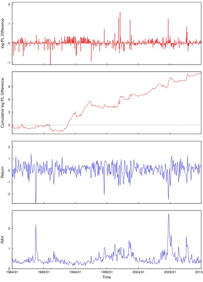
Figures 1 gives a breakdown of the period-by-period difference in the predictive likelihood values. Positive values are in favour of the model with RVt. The overall sum of the
log-predictive likelihoods is not due to a few outliers or any one period but represent ongoing improvements in accuracy. The joint models do a better job in forecasting return densities when the market is in a high volatility period, such as the period of 1973-1974 crash, the period before and after the internet bubble and the 2008 financial crisis.
6.1.2 Parameter Estimates and State Inference
Table 5 reports the posterior summary of parameters of the 2 state MS, MS-RV and MS-RAV models based on the full sample. To avoid label switching issues, we use informative priors
µ1 ∼N(-1,1), µ2 ∼N(1,1), P1 ∼Dir(4,1), P2 ∼Dir(1,4) andσj2 ∼IG(5,5) for j = 1,2 and
restrict µ1 < 0 and µ2 > 0.8 The results show that all three models are able to sort stock
returns into two regimes. One regime has a negative mean and high volatility, the other regime has positive mean return mean along with lower variance. This is consistent with the results of Maheu et al. (2012) and several other studies.
Compared with the benchmark MS model, the joint models specify the return distribution more precisely in each state, as can be seen the smaller estimated values σ2
st. For instance,
in the first state the innovation variance is 1.6127 for the MS model, while the estimates
of variance are 0.5633 and 0.6581 in the MS-RV and MS-RAV models, respectively. The variance estimates in the positive mean regimes drop from 0.2187 to 0.1556 and 0.1460 after joint modelling RV and RAV. We would expect this reduction in the innovation variance to result in better forecasts which is what we found in the previous section.
Another interesting result is that MS-RV and MS-RAV models provide more precise estimates of all the model parameters. As shown in Table 5, all the parameter estimators have smaller posterior standard deviations and shorter 0.95 density intervals. For example, the length of the density interval of µ1 from the benchmark model is 0.437, while the values
are 0.187 and 0.167 from the MS-RV and MS-RAV models, respectively. Figure 2 plots Eσst2y1:T
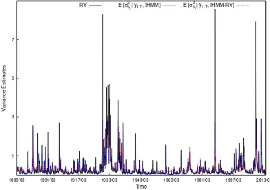
for the IHMM-RV and IHMM models. Volatility estimates vary over a larger range from the IHMM-RV model. For example, it appears that the IHMM overestimates the return variance during calm market periods and underestimates the return variance in several high volatile periods, such as the October 1987 crush and the financial crisis in 2008. In contrast, the return variance from the IHMM-RV model is closer to RV during these times. The differences between the models is due to the additional information from ex post volatility.
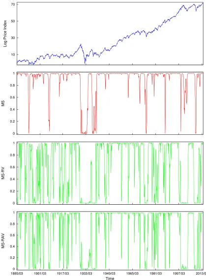
Figure 3 plots of smoothed probability of the high return state from the 2 state MS, MS-RV and MS-RAV models. The benchmark MS model does a fairly good job in identifying the primary downward market trends, such as the big crash of 1929, 1973-1974 bear market and the 2008 market crash, but it ignores a series of panic periods before and after 1900, the internet bubble crash and several other relatively smaller downward periods. The joint MS-RV and MS-RAV models not only identify the primary market trends but also are able to capture a number of short lived market drops. The main difference is that the joint model appears to have more frequent state switches and state identification is more precise. One obvious example is the joint models identify the dot-com collapse from 2000 to 2002 and the market crash of 2008-2009.
In summary, the joint models lead to better density forecasts, better forecasts of realized variance, improved parameter precision and minor differences in latent state estimates.
6.2
Foreign Exchange
The second example is using exchange rates between Canadian dollar (CAD) and U.S. dollar (USD). The exchange rate is in the unit of U.S. dollar and span from September 1971 to December 2013 (518 observations). The data source is Pacific Exchange Rate Service.9
The daily exchange rates Pt are first converted into continuous compound percentage
returns by rt = 100×(logPt−logPt−1) from which monthly returns and monthly volatility
measures are derived. Table 6 report summary statistics for monthlyrt,RVt, log(RVt),RAVt
and log(RAVt) for CAD/USD rates.
6.2.1 Out-of-Sample Forecasts
Table 7 displays the model comparisons results. The model priors are all relatively uninfor-mative and same as in the previous application. The out-of-sample period is from January
1991 to December 2013 (276 observations). According to the sum of log-predictive likeli-hoods, the proposed joint MS and infinite hidden Markov models outperform the benchmark models. Moving from the benchmark model to the joint specification can result in a sub-stantial gain. For instance, the log-predictive likelihood increases by 15.77 in moving from MS to MS-RV for the 3 state specification. The IHMM-RV model has the highest predictive likelihood among all other models. In addition, all the joint models produce better forecasts of realized variance. The improvements in the RMSE of RVt are often better than 5%.
7
Multivariate Return Applications
Two examples of the joint MS-RCOV models are considered. The prior specification is found in Table 8.
7.1
Equity
The data are constructed from daily continuously compounded returns on IBM, XOM and GE obtained from CRSP. The monthly RCOV is computed using daily values following equation (3). The summary statistics of monthly returnsRtandRCOVtare found in Table 9.
The data range from January 1926 to December 2013 (1056 observations)
7.1.1 Out-of-Sample Forecasts
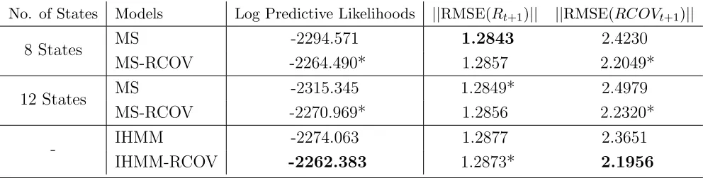
Table 10 reports the results of density forecasts and the root mean squared error of predictions based on 756 out-of-sample observations. We found the larger finite state models are the most competitive and therefore do not include results for small dimension models. The 8 and 12 state models that exploit RCOV are all superior to the models that do not according to log-predictive values. The improvement in the log-predictive likelihood is 30 or more. Further improvements are found on moving to the Bayesian nonparametric models. The IHMM-RCOV model is the best over the alternative models.
As for point predictions of return and realized covariance, the results is similar to the univariate return applications. The proposed joint models improve predictions of RCOVt
but offer no gains for return predictions.
Figure 4 displays the posterior average of active states in both IHMM and IHMM-RCOV models at each point in the out-of-sample period. It shows that more states are used in the joint return-RCOV model in order to better capture the dynamics of returns and volatility.
7.2
Foreign Exchange
The data are the exchange rates between U.S. dollar (USD) and 3 currencies (Canadian dollar (CAD), British pounds (GBP) and Japanese Yen (JPY)). The monthly RCOVt is
computed using daily exchange rates following equation (3). The summary statistics of monthly returns and RCOVt are found in Table 11. The data range from October 1971 to
7.2.1 Out of Sample Forecasts
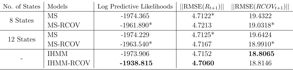
The out-of-sample period is January 1991 to December 2013 (276 observations). Results are found in Table 12. A bivariate and trivariate example are considered. Once again the joint models that use RCOV uniformly improve on density forecasts, and generally but not always, reduce the RSME for RCOVt forecasts. The overall best model according to the
predictive likelihood is the IHMM-RCOV specification. Predictive Bayes factors against any of the alternatives is substantial.
8
Conclusion
9
Appendix
9.1
MS-RV
(1) s1:T
y1:T, θ, φ, P
The latent state variables1:T is sampled using the forward filter backward sampler (FFBS)
in Chib (1996). The forward filter part contains the following steps.
i. Set the initial value of filter p(s1 =j
y1, θ, φ, P) = πj, forj = 1, . . . , K, where π is the
stationary distribution, which can be computed by solving π=P⊺π.
ii. Prediction step: p(st
y1:t−1, θ, φ, P)∝ PK
j=1Pj,st ·p(st−1 =j
y1:t−1, θ, φ, P).
iii. Update step:
p(st
y1:t, θ, φ, P)∝f(rt
µst, σst2)·g(RVt
ν+ 1, νσst2)·p(st
y1:t−1, θ, φ, P),
where f(·) and g(·) denote normal density and inverse gamma density, respectively.
The underlying states are drawn using backward sampler as follows.
i. For t =T, draw sT from p(sT
y1:T, θ, φ, P).
ii. For t =T −1, . . . ,1, draw st from Pst,st+1·p(st
y1:t, θ, φ, P).
Let nj = PT
t=11(st=j) denotes the number of observations belong to state j.
(2) µj
r1:T, s1:T, σj2 for j = 1, . . . , K
µj is sampled using Gibbs sampling for the linear regression model. Given prior µj ∼
N(mj, vj2), µj is sampled from conditional posterior N(mj, vj2), where
mj =
v2jPst=jrt+mjσj2 σj2+njvj2
, and vj2 =
σj2vj2 σ2j +njv2j
.
(3) σj2y1:T, µj, ν, s1:T for j = 1, . . . , K
The prior of σ2j is assumed to beσj2 ∼G(v0, s0). The conditional posterior of σj2 is given
as follows,
p(σ2jy1:T, µj, ν, s1:T) ∝ Y
st=j
1
σj
exp
−(rt−µj)
2
2σj2
·(νσj2)(ν+1)exp
−νσ 2 j RVt
·(σj2)v0−1
exp −s0σj2
.
The conditional posterior of σj2 is not of any known form, therefore Metropolis-Hasting algorithm is applied to sampleσ2
j. Combining theRV likelihood function and prior provides
the following good proposal density
σ2j ∼ G nj(ν+ 1) +v0, ν
X
st=j
1
RVt
+s0
(4) νy1:T,{σj2}Kj=1, s1:T
The prior of ν is assumed to beν ∼IG(a, b). The posterior of ν is given as follows.
p(νy1:T, σ2st, s1:T)∝ T Y
t=1
(
(νσst2)(ν+1)
Γ(ν+ 1) RV
−ν−2
t exp −νσ 2 st RVt )
·(ν)−a−1
exp
−νb
and ν is drawn from a random walk proposal with negative draws being rejected.
(5) Ps1:T
Using conjugate prior for rows of the transition matrix P: Pj ∼ Dir(αj1,· · · , αjK), the
posterior is given by Dir(αj1+mj1,· · · , αjK+mjK), where vector (mj1, mj2,· · · , mjK) records
the numbers of switches from state j to the other states.
9.2
MS-logRV
Forward filter backward filter is used to sample s1:T. The sampling ofP is the same as step
(5) in MS-RV model estimation. The sampling of µj is same as step (2) in MS-RV model
except replacing σj2 with exp(ζj).
Assuming the prior ζj ∼N(mζ,j, vζ,j2 ), the conditional posterior of ζj is given as follows,
p(ζj
y1:T, µj, δj2, s1:T) ∝ Y
st=j (
exp
−ζ2j − (rt−µj)
2
2 exp(ζj)
·exp
"
−(logRVt−ζj+
1 2δ
2
j)2
2δj2
#)
·exp
"
−(ζj−mζj)
2
2v2
ζ,j #
Metropolis-Hasting algorithm is applied to sample ζj. The proposal density is based on a
Gaussian approximation, so that ζj ∼N(µ∗∗j , σ
∗2
j ) where
µ∗
j =
v2
ζ,j P
st=jlog(RVt) +
1
2njvζ2δ2j +δj2mζ,j njvζ,j2 +δj2
, σ∗2
j =
δj2vζ,j2 njvζ,j2 +δj2
,
µ∗∗
j =µ
∗ +1 2σ ∗2 " X
st=j
(rt−µj)2exp(−µ ∗
)−nj #
.
Using conjugate prior δj2 ∼IG(v0, s0), the posterior density of δj2 is given by
p(δj2y1:T, µj, σj2) ∝ Y
st=j (
1
δj
exp
"
−(logRVt−ζj+
1 2δ
2
j)2
2δj2
#)
·δ−v0−1
j exp
−sδ02
j
A Metropolis-Hasting step is used to sample δj with the following proposal
δ2j ∼IG nj 2 +v0,
P
st=j(logRVt−ζj)
2
2 +s0
9.3
MS-RAV
The sampling step of s1:T, {µj}Kj=1 and P are same as in MS-RV model estimation. {σj}Kj=1
and ν are sampled as follows. With the prior σj2 ∼G(v0, s0) the conditional posterior of σj2
is,
p(σ2jy1:T, µj, ν, s1:T) ∝ Y
st=j (
1
σj
exp
−(rt−µj)
2
2σ2
j
·σj2νexp
" −
σjΓ(ν)
Γ(ν− 12)
2
1
RAV2
t #)
·(σ2j)v0−1
exp −s0σj2
The proposal distribution as a random walk.
Given ν ∼IG(a, b) the posterior of ν is given as follows,
p(νRAV1:T,{σj2}Kj=1, s1:T) ∝ T Y
t=1
(
σjΓ(ν)
Γ(ν− 12)
2ν
RAV−2ν−1 t
Γ(ν) exp
" −
σjΓ(ν)
Γ(ν−12)
2
1
RAV2
t #)
·ν−a−1
exp
b ν
A random walk proposal is used to sample ν and negative values are rejected.
9.4
MS-logRAV
The estimation of MS-logRAV model is very similar to that of MS-logRV model except changing the return variance exp(ζst) to exp(2ζst).
9.5
MMS-RCOV
See steps (1) and (5) in Section 9.1 for the sampling of s1:T and P.
Given conjugate prior Mj ∼N(Gj, Vj), the posterior density of Mj is given by
Mj
R1:T, s1:T,Σj ∼N(M , V), where
V = Σ−1 j nj+V
−1
j −1
, M =V Σ−1 j
X
st=j
Rt+GjV
−1
j !
.
The prior of Σj is assumed to be Σj ∼W(Ψ, τ). The conditional posterior of Σj is given as
follows,
p(Σj
Y1:T, Mj, ν, s1:T) ∝ Y
st=j
|Σj|
−1
2 exp
−12(Rt−Mj)⊺Σ
−1
j (Rt−Mj)
·Y
st=j
|Σj| ν
2|RCOVt|−
ν+d+1 2 exp
−12tr(ΣjRCOV
−1
t )
·|Σj| τ−d−1
2 exp
−12tr(Ψ−1
A Metropolis-Hasting algorithm is applied to sample Σj with proposal distribution
Σj ∼ W "
(ν−1−d)X
st=j
RCOV−1
t + Ψ
−1
#−1
, njν+τ .
Assuming prior of ν ∼G(a, b), the posterior density of ν is given as follows,
p(νY1:T, Mst,Σst, S)∝ T Y
t=1
|Σst(ν−d−1)| ν
2
2νd2 Γ(ν
2)
|RCOVt|
−ν+d+1
2
·exp
−12tr (ν−d−1)ΣstRCOV
−1
t
·νa−1
exp(−bν)
from which a random walk proposal is used to sample ν.
9.6
IHMM-RV
In the following if there are K active states (at least one observation is assigned to a state) then we keep track of the following truncated parameters: Γ = (γ1, . . . , γK, γKr+1),
Pj = (Pj,1, . . . , Pj,K, Pj,Kr +1) for j = 1, . . . , K. The terms γKr+1 and Pj,Kr +1 are residual
prob-ability terms that ensure the probprob-ability sums to one but are otherwise unused. Similarly we keep track of θ = (θ1, . . . , θK). Each of these vectors/matrix will expand or shrink as K
changes each iteration. In addition, define C= (c1, . . . , cK) and theK×K matrixA, which
will be used in sampling Γ and η. Several estimation steps are based on Maheu & Yang (2015) and Song (2014).
(1) u1:T
s1:T,Γ, P
Draw u1 ∼Uniform(0, γs1) and draw ut ∼Uniform(0, Pst−1,st) for t= 2, . . . , T.
(2) Adjust the number of states K
i. Check if max{Pr
1,K+1,· · · , PK,Kr +1}>min{u1:T}. If yes, expand the number of clusters
by making the following adjustments (ii) - (vi), otherwise, move to step (3).
ii. Set K =K+ 1.
iii. Draw uβ ∼ Beta(1, η), set γK = uβγKr and the new residual probability equals to γKr+1 = (1−uβ)γKr.
iv. For j = 1,· · · , K, draw uβ ∼ Beta(γK, γK+1), set Pj,K = uβPj,Kr and Pj,Kr +1 = (1−
uβ)Pj,Kr . Add an additional row to transition matrix P. PK+1 ∼Dir(αγ1,· · · , αγK).
v. Expand the parameter θ by one element by drawing µK+1 ∼ N(m, v2) and σK2+1 ∼
IG(v0, s0).
(3) s1:T|y1:T, u1:T, θ, φ, P,Γ
In this step, the latent state variable is sampled using the forward filter backward sampler (Chib 1996). The forward filter part contains the following steps:
i. Set the initial value of filter p(st =j
y1, u1, θ, φ, P) =1(u0 < γj) and normalize it.
ii. Prediction step:
p(st
y1:t−1, u1:t−1, θ, φ, P)∝ K X
j=1
1(ut< Pj,st)·p(st−1 =j
y1:t−1, u1:t−1, θ, φ, P).
iii. Update step:
p(st
y1:t, u1:t, θ, φ, P)∝f(rt
µj, σj2)·g(RVt
ν+ 1, νσj2)·p(st
y1:t−1, u1:t−1, θ, φ, P).
The underlying states are drawn using backward sampler as follows.
i. For t =T, draw sT from p(sT
y1:T, u1:T, θ, φ, P).
ii. For t =T −1,· · · ,1, draw st from1(ut< Pj,st+1)·p(st
y1:t, u1:t, P, θ, φ).
Then we count the number of active clusters and remove inactive states by making following adjustments.
i. Calculate the number of active states (denoted by L). If L < K, remove the inactive states and relabel states from 1 to L.
ii. Adjust the order of state-dependent parameters µ, σ2 and Γ according to the adjusted
state s1:T.
iii. SetK =L. Recalculate the residual probabilities of Γr
K+1 for j = 1,· · · , K. Then set
the values of parameterµj, σj2 and γj, to be zero for j > K.
(4) Γs1:T, η, α
i. Let nj,i denotes the number of state moves from state j to i. Calculate nj,i for i =
1,· · ·, K and j = 1,· · · , K.
ii. For i = 1,· · · , K and j = 1,· · · , K, if nj,i > 0, then for l = 1,· · · , nj,i, draw xl ∼
Bernoulli(l−1+αγiαγi). If xl= 1, set Aj,i =Aj,i+ 1.
iii. Draw Γ∼Dir(c1, . . . , cK, η), where ci = PK
j=1Aji.
(5) Ps1:T,Γ, α
For j = 1,· · ·K, draw Pj ∼Dir(αγ1+nj,1,· · ·, αγk+nj,K, αγKr+1).
See the step (2) and step (3) in Appendix 9.1. for the estimation of state-dependent parameters µj, σ2j, forj = 1, . . . , K.
(7) νy1:T, s1:T,{σj2}Kj=1, ν
Same as the step (4) in Appendix 9.1.
(8) ηs1:T,Γ, α
Recompute C following step (4) and define ν and λ, whereν ∼Bernoulli(PPKi=1ci
K
i=1ci+η) and
λ∼Beta(η+ 1,PKi=1ci). Then draw a new value of η∼G(a1+K−ν, b1−log(λ)).
(9) αs1:T, C
Define ν′ j, λ
′
j, for j = 1,· · · , K, where ν ′
j ∼ Bernoulli(
PK i=1nj,i
PK
i=1nj,i+α) and λ
′
j ∼ Beta(α+
1,PKi=1nj,i). Then draw α∼G(a2+PKj=1cj− PK
j=1ν
′
j, b2−PKj=1log(λ
′ j)).
9.7
IHMM-logRV and IHMM-logRAV
See step (1) - (5), (8) and (9) in Appendix 9.6 for the sampling of the auxiliary variable
u1:T, latent state variables1:T, Γ, transition matrixP, DP concentration parameterηand α.
The sampling of θ = {µj, ζj, δj2} ∞
j=1 in IHMM-logRV are same as the MS-logRV model, see
Appendix 9.3. The posterior sampling for the IHMM-logRAV model can be done similarly.
9.8
IHMM-RCOV
See step (1) - (5), (8) and (9) in Appendix 9.6 for the sampling of u1:T, s1:T, Γ, P, η and α. The sampling of θ ={Mj,Σj}
∞
j=1 and ν are same as in the MS-RCOV model, see section
References
Andersen, T. & Benzoni, L. (2009), Realized volatility, in ‘Handbook of Financial Time Series’, Springer.
Andersen, T. G., Bollerslev, T., Diebold, F. X. & Ebens, H. (2001), ‘The distribution of realized stock return volatility’,Journal of Financial Economics 61(1), 43–76.
Ang, A. & Bekaert, G. (2002), ‘Regime Switches in Interest Rates’, Journal of Business & Economic Statistics 20(2), 163–82.
Barndorff-Nielsen, O. E. & Shephard, N. (2002), ‘Estimating quadratic variation using real-ized variance’, Journal of Applied Econometrics17, 457–477.
Barndorff-Nielsen, O. E. & Shephard, N. (2004a), ‘Econometric Analysis of Realized Co-variation: High Frequency Based Covariance, Regression, and Correlation in Financial Economics’, Econometrica 72(3), 885–925.
Barndorff-Nielsen, O. E. & Shephard, N. (2004b), ‘Power and bipower variation with stochas-tic volatility and jumps’, Journal of Financial Econometrics 2, 1–48.
Carpantier, J.-F. & Dufays, A. (2014), Specific markov-switching behaviour for arma pa-rameters, CORE Discussion Papers 2014014, Universit catholique de Louvain, Center for Operations Research and Econometrics (CORE).
Chib, S. (1996), ‘Calculating posterior distributions and modal estimates in markov mixture models’, Journal of Econometrics 75(1), 79–97.
Dueker, M. & Neely, C. J. (2007), ‘Can Markov switching models predict excess foreign exchange returns?’, Journal of Banking & Finance31(2), 279–296.
Dufays, A. (2012), Infinite-state markov-switching for dynamic volatility and correlation models, CORE Discussion Papers 2012043, Universit catholique de Louvain, Center for Operations Research and Econometrics (CORE).
Engel, C. & Hamilton, J. D. (1990), ‘Long swings in the dollar: Are they in the data and do markets know it?’, American Economic Review 80, 689–713.
Ferguson, T. S. (1973), ‘A bayesian analysis of some nonparametric problems’, The Annals of Statistics 1(2), 209–230.
Gael, J. V., Saatci, Y., Teh, Y. W. & Ghahramani, Z. (2008), Beam sampling for the infinite hidden markov model, in ‘In Proceedings of the 25th International Conference on Machine Learning’.
Guidolin, M. & Timmermann, A. (2008), ‘International asset allocation under regime switch-ing, skew, and kurtosis preferences’, Review of Financial Studies 21(2), 889–935.
Hamilton, J. D. (1989), ‘A New Approach to the Economic Analysis of Nonstationary Time Series and the Business Cycle’, Econometrica57(2), 357–84.
Jochmann, M. (2015), ‘Modeling U.S. Inflation Dynamics: A Bayesian Nonparametric Ap-proach’, Econometric Reviews34(5), 537–558.
Kim, C.-J., Morley, J. C. & Nelson, C. R. (2004), ‘Is there a positive relationship between stock market volatility and the equity premium?’,Journal of Money, Credit and Banking
36(3), pp. 339–360.
Lunde, A. & Timmermann, A. G. (2004), ‘Duration dependence in stock prices: An analysis of bull and bear markets’, Journal of Business & Economic Statistics 22(3), 253–273.
Maheu, J. M. & McCurdy, T. H. (2000), ‘Identifying bull and bear markets in stock returns’,
Journal of Business & Economic Statistics 18(1), 100–112.
Maheu, J. M., McCurdy, T. H. & Song, Y. (2012), ‘Components of bull and bear markets: Bull corrections and bear rallies’,Journal of Business & Economic Statistics30(3), 391– 403.
Maheu, J. M. & Yang, Q. (2015), An Infinite Hidden Markov Model for Short-term Interest Rates, Working Paper Series 15-05, The Rimini Centre for Economic Analysis.
Pastor, L. & Stambaugh, R. F. (2001), ‘The Equity Premium and Structural Breaks’,Journal of Finance 56(4), 1207–1239.
Schwert, G. W. (1990), ‘Indexes of u.s. stock prices from 1802 to 1987’, Journal of Business
63(3), 399–426.
Song, Y. (2014), ‘Modelling regime switching and structural breaks with an infinite hidden markov model’,Journal of Applied Econometrics 29(1), 825–842.
Takahashi, M., Omori, Y. & Watanabe, T. (2009), ‘Estimating stochastic volatility models using daily returns and realized volatility simultaneously’, Computational Statistics & Data Analysis 53(6), 2404–2426.
Teh, Y. W., Jordan, M. I., Beal, M. J. & Blei, D. M. (2006), ‘Hierarchical dirichlet processes’,
Journal of the American Statistical Association 101(476), pp. 1566–1581.
Walker, S. G. (2007), ‘Sampling the dirichlet mixture model with slices’, Communications in Statistics - Simulation and Computation 36(1), 45–54.
Table 1: Prior Specifications of Univariate Return Models
Panel A: Priors for MS and Joint MS Models
Model µst σst2 ν δ2st Pj
MS N(0,1) IG(2,var(c rt)) - Dir(1, . . . ,1)
MS-RV N(0,1) G(RVt,1) IG(2,1) Dir(1, . . . ,1)
MS-RAV N(0,1) G(RVt,1) IG(2,1) Dir(1, . . . ,1)
MS-logRV N(0,1) N(log(RVt),5) - IG(2,0.5) Dir(1, . . . ,1)
MS-logRAV N(0,1) N(log(RAVt),5) - IG(2,0.5) Dir(1, . . . ,1)
Panel B: Priors for IHMM and Joint IHMM Models
Model µst σst2 ν δ2st η α
IHMM N(0,1) IG(2,var(c rt)) - - G(1,4) G(1,4)
IHMM-RV N(0,1) G(RVt,1) IG(2,1) - G(1,4) G(1,4)
IHMM-logRV N(0,1) N(log(RVt),5) - IG(2,0.5) G(1,4) G(1,4)
IHMM-logRAV N(0,1) N(log(RAVt),5) - IG(2,0.5) G(1,4) G(1,4)
c
[image:28.612.96.514.408.509.2]var(rt) is the sample variance,RVt, log(RVt) and log(RAVt) are the sample means. All are computed using in-sample data.
Table 2: Summary Statistics for Monthly Equity Returns and Volatility Measures
Data Mean Median Stdev Skewness Kurtosis Min Max
rt 0.047 0.097 0.612 -0.539 9.123 -4.154 3.884 RVt 0.328 0.156 0.621 6.853 68.499 0.010 8.580 RAVt 0.470 0.394 0.287 2.807 14.358 0.103 2.747
log(RVt) -1.720 -1.856 0.964 0.714 3.992 -4.608 2.149
Table 3: Equity Forecasts: 1951-2013
No. of States Models Log-predicitive Likelihoods RMSE[rt+1] RMSE[RVt+1]
2 States
MS -548.409 0.5268 0.5285 MS-RV -535.003 0.5242* 0.5338 MS-logRV -534.914 0.5276 0.5229 MS-RAV -533.370* 0.5263 0.5263 MS-logRAV -534.256 0.5269 0.5199*
3 States
MS -538.437 0.5244* 0.5240 MS-RV -523.000* 0.5290 0.5070 MS-logRV -524.754 0.5286 0.5087 MS-RAV -523.171 0.5276 0.5032* MS-logRAV -525.353 0.5283 0.5048
4 States
MS -535.454 0.5232* 0.5193 MS-RV -520.363* 0.5273 0.5029 MS-logRV -528.631 0.5284 0.4902* MS-RAV -527.708 0.5277 0.4976 MS-logRAV -530.697 0.5290 0.4920
-IHMM -535.165 0.5229 0.5348 IHMM-RV -514.662 0.5216 0.4724 IHMM-logRV -516.643 0.5228 0.4647
IHMM-logRAV -517.148 0.5244 0.4775
This table reports the sum of 1-period ahead log-predictive likelihoods of return
PT
j=t+1log(p(rj|y1:j−1,Model)), root mean squared error for return and realized variance
Table 4: Equity Forecasts: 1984-2013
No. of States Models Log-Predictive Likelihoods RMSE[rt+1] RMSE[RVt+1]
2 States
MS -300.019 0.5542 0.6863 MS-RV -293.311 0.5512* 0.7130 MS-logRV -291.794 0.5563 0.6938* MS-RAV -290.353* 0.5543 0.7050 MS-logRAV -290.709 0.5553 0.6968
3 States
MS -294.914 0.5522* 0.6817 MS-RV -283.877 0.5570 0.6794 MS-logRV -284.135 0.5568 0.6781 MS-RAV -281.126* 0.5556 0.6764* MS-logRAV -282.150 0.5561 0.6772
4 States
MS -292.397 0.5506* 0.6755 MS-RV -281.211* 0.5553 0.6749 MS-logRV -285.383 0.5570 0.6564* MS-RAV -282.523 0.5559 0.6696 MS-logRAV -284.563 0.5580 0.6614
-IHMM -291.091 0.5529 0.7002 IHMM-RV -279.504 0.5475 0.6344 IHMM-logRV -281.344 0.5503 0.6209
IHMM-logRAV -280.019 0.5529 0.6434
This table reports the sum of 1-period ahead log-predictive likelihoods of return
PT
j=t+1log(p(rj|y1:j−1,Model)), root mean squared error for return and realized variance
Table 5: Estimates for Stock Market Returns
MS MS-RV MS-RAV Parameter Mean Stdev Mean Stdev Mean Stdev
µ1 -0.2995 0.1104 -0.0840 0.0354 -0.1372 0.0445
(-0.528, -0.089) (-0.159, -0.020) (-0.229, -0.050)
µ2 0.0875 0.0140 0.1224 0.0139 0.1130 0.0125
(0.060, 0.116) (0.096, 0.149) (0.089, 0.138)
σ2 1
1.6127
0.2630 0.5633 0.0486 0.6581 0.0394
(1.191, 2.217) (0.481, 0.678) (0.597, 0.748)
σ22 0.2187 0.0115 0.1556 0.0049 0.1460 0.0044
(0.196, 0.241) (0.143, 0.171) (0.138, 0.154)
ν - - 1.3431 0.0824 2.1529 0.0758
(1.183, 1.501) (2.009, 2.316)
P1,1 0.8775 0.0396 0.9023 0.0193 0.8716 0.0210
(0.793, 0.943) (0.862, 0.937) (0.828, 0.910)
P2,2 0.9849 0.0058 0.9442 0.0099 0.9538 0.0083
(0.972, 0.994) (0.924, 0.962) (0.937, 0.969)
This table reports the posterior mean, standard deviation and 0.95 density intervals (values in brackets) of parameters of selected 2 state models. The prior restriction µ1 <0 and µ2>0 is
imposed. The sample period is from March 1885 to December 2013 (1542 observations).
Table 6: Summary Statistics of CAD/USD Rate and ex-post Volatility Measures
Data Mean Median Stdev Skewness Kurtosis Min Max
rt -0.018 0.000 1.840 -0.669 10.485 -13.780 8.555 RVt 3.299 1.610 6.272 7.336 76.883 0.032 80.301
log(RVt) 0.436 0.476 1.239 -0.089 3.153 -3.442 4.386 RAVt 1.476 1.233 0.998 2.339 12.654 0.174 8.962
[image:31.612.100.512.540.642.2]Table 7: CAD/USD Forecasts
No. of States Models Log-Predictive Likelihoods RMSE[rt+1] RMSE[RVt+1]
3 States
MS -610.836 2.2475* 7.8459 MS-RV -595.066 2.2528 7.5441 MS-logRV -593.358* 2.2515 7.4586* MS-RAV -603.318 2.2510 7.6179 MS-logRAV -598.427 2.2528 7.5262
4 States
MS -612.228 2.2431 7.9947 MS-RV -593.145 2.2539 7.5243 MS-logRV -590.109* 2.2583 7.2245* MS-RAV -596.065 2.2580 7.4700 MS-logRAV -596.698 2.2612 7.3397
-IHMM -603.772 2.2695 7.7002 IHMM-RV -586.815 2.2580* 7.2399 IHMM-logRV -585.591 2.2646 7.4938 IHMM-logRAV -590.079 2.2702 7.1122
This table summarizes the sum of 1-period ahead log predictive likelihoods of CAD/USD rate
PT
j=t+1log(p(rj|y1:j−1,Model)), root mean squared errors of mean and variance prediction of
CAD/USD rates over period from Jan 1991 to Dec 2013 (276 observations).
Table 8: Prior Specification of Multivariate Models
Panel A: Priors for Multivariate MS Models Model Mst Σst ν Pj
MS N(0,5I) IW(Cov(d Rt),5) - Dir(1, . . . ,1)
MS-RCOV N(0,5I) W(1
3RCOVt,3) G(20,1)1ν>4 Dir(1, . . . ,1)
Panel B: Priors for Multivariate IHMM Models
Model Mst Σst ν η α
IHMM N(0,5I) IW(Cov(d Rt),5) - G(1,4) G(1,4)
IHMM-RCOV N(0,5I) W(1
3RCOVt,3) G(20,1)1ν>4 G(1,4) G(1,4)
[image:32.612.83.526.523.665.2]Table 9: Summary Statistics of Returns (IBM, XOM, GE)
Panel A: Summary of Returns
Data Mean Median St. Dev Skewness Kurtosis Min Max IBM 0.134 0.135 0.824 -0.192 5.169 -3.644 3.635 XOM 0.116 0.096 0.707 -0.152 6.942 -3.930 3.773 GE 0.103 0.088 0.940 -0.324 7.755 -5.265 5.336
Panel B: Return Covariance and RCOV mean Covariance of Return Average of RCOV Data IBM XOM GE IBM XOM GE IBM 0.678 0.236 0.411 0.742 0.250 0.370 XOM 0.236 0.500 0.338 0.250 0.641 0.394 GE 0.411 0.338 0.882 0.370 0.394 0.970
The panel A of above table reports the summary statistics of the monthly return of IBM, XOM and GE. The reported data are annualized values after scaling the raw returns by 12. The panel B reports the covariance matrix calculated from monthly return vectors and the averaged RCOV matrix, which are calculated using daily returns. The sample period is from Jan 1926 to Dec 2013 (1056 observations).
Table 10: Multivariate Equity Forecasts
No. of States Models Log Predictive Likelihoods ||RMSE(Rt+1)|| ||RMSE(RCOVt+1)||
8 States MS -2294.571 1.2843 2.4230 MS-RCOV -2264.490* 1.2857 2.2049*
12 States MS -2315.345 1.2849* 2.4979 MS-RCOV -2270.969* 1.2856 2.2320*
- IHMM -2274.063 1.2877 2.3651 IHMM-RCOV -2262.383 1.2873* 2.1956
This table summarizes the sum of 1 month log predictive likelihoods of return,PTj=t+1log(p(Rj|y1:j−1,Model)),
root mean squared errors of mean and covariance prediction over Jan 1951 to Dec 2013 (totally 756 predictions), when the models are applied to analyze IBM, XOM, GE jointly. The root mean squared errors provided in this table are matrix norms. ||A||=qPiPja2
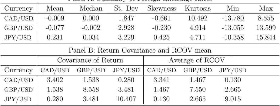
[image:33.612.72.568.502.628.2]Table 11: Summary Statistics of Foreign Exchange Rates (CAD/USD, GBP/USD, JPY/USD)
Panel A: Summary of Foreign Exchange Rates
Currency Mean Median St. Dev Skewness Kurtosis Min Max
CAD/USD -0.009 0.000 1.847 -0.661 10.492 -13.780 8.555
GBP/USD -0.077 -0.002 2.928 -0.230 4.914 -13.055 13.599
JPY/USD 0.231 0.034 3.229 0.425 4.711 -10.358 15.844
Panel B: Return Covariance and RCOV mean Covariance of Return Average of RCOV
Currency CAD/USD GBP/USD JPY/USD CAD/USD GBP/USD JPY/USD
CAD/USD 3.402 1.538 0.280 3.341 1.467 0.130
GBP/USD 1.538 8.558 3.481 1.467 7.550 2.665
JPY/USD 0.280 3.481 10.407 0.130 2.665 9.015
Table 12: Multivariate Foreign Exchange Forecasts
2 Assets Case: CAD/USD and GBP/USD
No. of States Models Log Predictive Likelihoods ||RMSE(Rt+1)|| ||RMSE(RCOVt+1)||
4 States MS -1257.766 3.5184 13.4125* MS-RCOV -1249.800* 3.5184* 13.8117
8 States MS -1265.918 3.5180 13.7968 MS-RCOV -1235.374* 3.5346 13.2523*
- IHMM -1250.196 3.5294* 13.0182 IHMM-RCOV -1222.628 3.5394 12.8453
3 Assets Case: CAD/USD, GBP/USD and JPY/USD
No. of States Models Log Predictive Likelihoods ||RMSE(Rt+1)|| ||RMSE(RCOVt+1)||
8 States MS -1974.365 4.7122* 19.4322 MS-RCOV -1961.890* 4.7213 19.0318*
12 States MS -1974.229 4.7125* 19.6424 MS-RCOV -1963.540* 4.7167 18.9910*
- IHMM -1973.906 4.7152 18.8065 IHMM-RCOV -1938.815 4.7060 18.8146
This table summarizes the sum of 1 month log predictive likelihoods of returnPTj=t+1log(p(Rj|y1:j−1,Model)),
root mean squared errors of return and covariance prediction over Jan 1991 to Dec 2013 (276 predictions). The root mean squared errors provided in this table are matrix norms. ||A||=qPiPja2
-1 0 1 2
log-PL Difference
0 3 6 9
Cumulative log-PL Difference
-2 -1 0 1 2
Return
0 1 2
1984/01 1989/01 1994/01 1999/01 2004/01 2009/01 2013/12
RAV
[image:36.612.94.510.68.644.2]Time
Figure 1: The top panel shows log (p(rt+1|y1:t,MS-RV))−log (p(rt+1|y1:t,MS)) over Jan 1984
1 3 5 7
1885/03 1901/03 1917/03 1933/03 1949/03 1965/03 1981/03 1997/03 2013/03
Variance Estimates
Time RV E [σ
st 2
| y1:T, IHMM] E [σ st 2
[image:37.612.107.499.79.355.2]| y1:T, IHMM-RV]
Figure 2: Eσ2sty1:T,IHMM
,Eσst2y1:T,IHMM-RV
10 30 50 70
Log Price Index
0 0.2 0.4 0.6 0.8 1
MS
0 0.2 0.4 0.6 0.8 1
MS-RV
0 0.2 0.4 0.6 0.8 1
1885/03 1901/03 1917/03 1933/03 1949/03 1965/03 1981/03 1997/03 2013/03
MS-RAV
[image:38.612.93.512.68.637.2]Time