A Sequential Matching Framework for Multi Turn Response Selection in Retrieval Based Chatbots

Retrieval-Based Chatbots

Yu Wu

Beihang University

State Key Laboratory of Software Development Environment [email protected]

Wei Wu

Microsoft Corporation Research and AI Group [email protected]

Chen Xing

College of Computer and Control Engineering

[email protected]

Can Xu

Microsoft Corporation Research and AI Group [email protected]

Zhoujun Li

State Key Laboratory of Software Development Environment [email protected]

Ming Zhou

Natural Language Computing Group [email protected]

Submission received: 14 August 2017; revised version received: 3 July 2018; accepted for publication: 6 December 2018.

We study the problem of response selection for multi-turn conversation in retrieval-based chatbots. The task involves matching a response candidate with a conversation context, the challenges for which include how to recognize important parts of the context, and how to model the relationships among utterances in the context. Existing matching methods may lose important information in contexts as we can interpret them with a unified framework in which contexts are transformed to fixed-length vectors without any interaction with responses before matching. This motivates us to propose a new matching framework that can sufficiently carry important information in contexts to matching and model relationships among utterances at the same time. The new framework, which we call a sequential matching framework (SMF), lets each utterance in a context interact with a response candidate at the first step and transforms the pair to a matching vector. The matching vectors are then accumulated following the order of the utterances in the context with a recurrent neural network (RNN) that models relationships among utterances. Context-response matching is then calculated with the hidden states of the RNN. Under SMF, we propose a sequential convolutional network and sequential attention network and conduct experiments on two public data sets to test their performance. Experiment results show that both models can significantly outperform state-of-the-art matching methods. We also show that the models are interpretable with visualizations that provide us insights on how they capture and leverage important information in contexts for matching.

1. Introduction

Recent years have witnessed a surge of interest on building conversational agents both in industry and academia. Existing conversational agents can be categorized into task-oriented dialog systems and non–task-task-oriented chatbots. Dialog systems focus on help-ing people complete specific tasks in vertical domains (Young et al. 2010), such as flight booking, bus route enquiry, restaurant recommendation, and so forth; chatbots aim to naturally and meaningfully converse with humans on open domain topics (Ritter, Cherry, and Dolan 2011). Building an open domain chatbot is challenging, because it requires the conversational engine to be capable of responding to any input from humans that covers a wide range of topics. To address the problem, researchers have considered leveraging the large amount of conversation data available on the Internet, and proposed generation-based methods (Shang, Lu, and Li 2015; Vinyals and Le 2015; Li et al. 2016b; Mou et al. 2016; Serban et al. 2016; Xing et al. 2017) and retrieval-based methods (Wang et al. 2013; Hu et al. 2014; Ji, Lu, and Li 2014; Wang et al. 2015; Yan, Song, and Wu 2016; Zhou et al. 2016; Wu et al. 2018a). Generation-based methods generate responses with natural language generation models learned from conversation data, while retrieval-based methods re-use the existing responses by selecting proper ones from an index of the conversation data. In this work, we study the problem of response selection in retrieval-based chatbots, because retrieval-based chatbots have the advantage of returning informative and fluent responses. Although most existing work on retrieval-based chatbots studies response selection for single-turn conversation (Wang et al. 2013) in which conversation history is ignored, we study the problem in a multi-turn scenario. In a chatbot, multi-turn response selection takes a message and utterances in its previous turns as an input and selects a response that is natural and relevant to the entire context.

matching where both the current message and the utterances in its previous turns should be taken into consideration. The challenges of the task include (1) how to extract important information (words, phrases, and sentences) from the context and leverage the information in matching; and (2) how to model relationships and dependencies among the utterances in the context. Table 1 uses an example to illustrate the challenges. First, to find a proper response for the context, the chatbot must know that “hold a drum class” and “drum” are important points. Without them, it may return a response relevant to the message (i.e., Turn-5 in the context) but nonsensical in the context (e.g., “what lessons do you want?”). On the other hand, words like “Shanghai” and “Lujiazui” are less useful and even noisy to response selection. The responses from the chatbot may drift to the topic of “Shanghai” if the chatbot pays significant attention to these words. Therefore, it is crucial yet non-trivial to let the chatbot understand the important points in the context and leverage them in matching and at the same time circumvent noise. Second, there is a clear dependency between Turn-5 and Turn-2 in the context, and the order of utterances matters in response selection because there will be different proper responses if we exchange Turn-3 and Turn-5.

Existing work, including the recurrent neural network architectures proposed by Lowe et al. (2015), the deep learning to respond architecture proposed by Yan, Song, and Wu (2016), and the multi-view architecture proposed by Zhou et al. (2016), may lose important information in context-response matching because they follow the same paradigm to perform matching, which suffers clear drawbacks. In fact, although these models have different structures, they can be interpreted with a unified framework: A context and a response are first individually represented as vectors, and then their matching score is computed with the vectors. The context representation includes two layers. The first layer represents utterances in the context, and the second layer takes the output of the first layer as an input and represents the entire context. The existing work differs in how they design the context representation and the response representation and how they calculate the matching score with the two representations. The framework view unifies the existing models and indicates the common drawbacks they have: everything in the context is compressed to one or more fixed-length vectors before matching is conducted; and there is no interaction between the context and the response in the formation of their representations. The context is represented without enough supervision from the response, and so is the response.

To overcome the drawbacks, we propose a sequential matching network (SMN) for context-response matching in our early work (Wu et al. 2017) where we construct

Table 1

An example of multi-turn conversation.

Context

Turn-1 Human: How are you doing?

Turn-2 ChatBot: I am going tohold a drum classin Shanghai. Anyone wants to join? The location is near Lujiazui.

Turn-3 Human: Interesting! Do you have coaches who can help me practice

drum?

Turn-4 ChatBot: Of course.

Turn-5 Human: Can I have a free first lesson?

Response Candidates

Response 1: Sure. Have you ever played drum before?X

a matching vector for each utterance–response pair through convolution and pooling on their similarity matrices, and then aggregate the sequence of matching vectors as a matching score of the context and the response. In this work, we take it one step further and generalize the SMN model to a sequential matching framework (SMF). The framework view allows us to tackle the challenges of context-response matching from a high level. Specifically, SMF matches each utterance in the context with the response at the first step and forms a sequence of matching vectors. It then accumulates the matching vectors of utterance–response pairs in the chronological order of the utter-ances. The final context-response matching score is calculated with the accumulation of pair matching. Different from the existing framework, SMF allows utterances in the context and the response to interact with each other at the very beginning, and thus important matching information in each utterance–response pair can be sufficiently preserved and carried to the final matching score. Moreover, relationships and depen-dencies among utterances are modeled in a matching fashion, so the order of utterances can supervise the aggregation of the utterance–response matching. Generally speaking, SMF consists of three layers. The first layer extracts important matching information from each utterance–response pair and transforms the information into a matching vector. The matching vectors are then uploaded to the second layer where a recurrent neural network with gated recurrent units (GRU) (Chung et al. 2014) is used to model the relationships and dependencies among utterances and accumulate the matching vectors into its hidden states. The final layer takes the hidden states of the GRU as input and calculates a matching score for the context and the response.

The key to the success of SMF lies in how to design the utterance–response matching layer, which requires identification of important parts in each utterance. We first show that the point-wise similarity calculation followed by convolution and pooling in SMN is one implementation of the utterance–response matching layer of SMF, making the SMN model a special case of the framework. Then, we propose a new model named sequential attention network (SAN), which implements the utterance–response match-ing layer of SMF with an attention mechanism. Specifically, for an utterance–response pair, SAN lets the response attend to important parts (either words or segments) in the utterance by weighting the parts using each part of the response. Each weight reflects how important the part in the utterance is with respect to the corresponding part in the response. Then for each part in the response, parts in the utterance are linearly combined with the weights, and the combination interacts with the part of the response by Hadamard product to form a representation of the utterance. Such utterance representations are computed on both a word level and a segment level. The two levels of representations are finally concatenated and processed by a GRU to form a matching vector. SMN and SAN are two different implementations of the utterance– response matching layer, and we give a comprehensive comparison between SAN and SMN. Theoretically, SMN is faster and easier to parallelize than SAN, whereas SAN can better utilize the sequential relationship and dependency. The empirical results are consistent with the theoretical analysis.

outperform the existing methods. Particularly, on the Ubuntu corpus, SMN and SAN yield 6 and 7 percentage point improvement, respectively, on R10@1 over the best

performing baseline method, and on the Douban corpus, the improvement on mean average precision from SMN and SAN over the best baseline are 2.6 and 3.6 percent-age points, respectively. The empirical results indicate that SAN can achieve better performance than SMN in practice. In addition to the quantitative evaluation, we also visualize the two models with examples from the Ubuntu corpus. The visualization reveals how the two models understand conversation contexts and provides us insights on why they can achieve big improvement over state-of-the-art methods.

This work is a substantial extension of our previous work reported at ACL 2017. The extension in this article includes a unified framework for the existing methods, a proposal of a new framework for context-response matching, and a new model under the framework. Specifically, the contributions of this work include the following.

• We unify existing context-response matching models with a framework and disclose their intercorrelations with detailed mathematical

derivations, which reveals their common drawbacks and sheds light on our new direction.

• We propose a new framework for multi-turn response selection, namely, the sequential matching framework, which is capable of overcoming the drawbacks suffered by the existing models and addressing the challenges of context-response matching in an end-to-end way. The framework indicates that the key to context-response matching is not the 2D convolution and pooling operations in SMN, but a general

utterance–response matching function that can capture the important matching information in utterance–response pairs.

• We propose a new architecture, the sequential attention network, under the new framework. Moreover, we compare SAN with SMN on both efficiency and effectiveness.

• We conduct extensive experiments on public data sets and verify that SAN achieves new state-of-the-art performance on context-response matching.

The rest of the paper is organized as follows: In Section 2 we summarize the related work. We formalize the learning problem in Section 3. In Section 4, we interpret the existing models with a framework. Section 5 elaborates our new framework and gives two models as special cases of the framework. Section 6 gives the learning objective and some training details. In Section 7 we give details of the experiments. In Section 8, we outline our conclusions.

2. Related Work

We briefly review the history and recent progress of chatbots, and application of text matching techniques in other tasks. Together with the review of existing work, we clarify the connection and difference between these works and our work in this article.

2.1 Chatbots

ELIZA needs huge human effort but can only return limited responses. To remedy this, researchers have developed data-driven approaches (Higashinaka et al. 2014). The idea behind data-driven approaches is to build a chatbot with the large amount of conversation data available on social media such as forums and microblogging services. Methods along this line can be categorized into retrieval-based and generation-based ones.

Generation-based chatbots reply to a message with natural language generation techniques. Early work (Ritter, Cherry, and Dolan 2011) regards messages and re-sponses as source language and target language, respectively, and learn a phrase-based statistical machine translation model to translate a message to a response. Recently, together with the success of deep learning approaches, the sequence-to-sequence frame-work has become the mainstream approach, because it can implicitly capture com-positionality and long-span dependencies in languages. Under this framework, many models have been proposed for both single-turn conversation and multi-turn conversa-tion. For example, in single-turn conversation, sequence-to-sequence with an attention mechanism (Shang, Lu, and Li 2015; Vinyals and Le 2015) has been applied to response generation; Li et al. (2016a) proposed a maximum mutual information objective to improve diversity of generated responses; Xing et al. (2017) and Mou et al. (2016) introduced external knowledge into the sequence-to-sequence model; Wu et al. (2018b) proposed decoding a response from a dynamic vocabulary; Li et al. (2016b) incorpo-rated persona information into the sequence-to-sequence model to enhance response consistency with speakers; and Zhou et al. (2018) explored how to generate emotional responses with a memory augmented sequence-to-sequence model. In multi-turn con-versation, Sordoni et al. (2015) compressed a context to a vector with a multi-layer per-ceptron in response generation; Serban et al. (2016) extended the sequence-to-sequence model to a hierarchical encoder-decoder structure; and under this structure, they further proposed two variants including VHRED (Serban et al. 2017b) and MrRNN (Serban et al. 2017a) to introduce latent and explicit variables into the generation process. Xing et al. (2018) exploited a hierarchical attention mechanism to highlight the effect of important words and utterances in generation. Upon these methods, reinforcement learning technique (Li et al. 2016c) and an adversarial learning technique (Li et al. 2017) have also been applied to response generation.

Different from the generation based systems, retrieval-based chatbots select a proper response from an index and re-use the one to reply to a new input. The key to response selection is how to match the input with a response. In a single-turn scenario, matching is conducted between a message and a response. For example, Hu et al. (2014) proposed message-response matching with convolutional neural networks; Wang et al. (2015) incorporated syntax information into matching; Ji, Lu, and Li (2014) combined several matching features, such as cosine, topic similarity, and translation score, to rank response candidates. In multi-turn conversation, matching requires taking the entire context into consideration. In this scenario, Lowe et al. (2015) used a dual long short-term memory (LSTM) model to match a response with the literal concatenation of utterances in a context; Yan, Song, and Wu (2016) reformulated the input message with the utterances in its previous turns and performed matching with a deep neural network architecture; Zhou et al. (2016) adopted an utterance view and a word view in matching to model relationships among utterances; and Wu et al. (2017) proposed a sequential matching network that can capture important information in contexts and model relationships among utterances in a unified form.

from a framework view, generalize the model in Wu et al. (2017) to a framework, give another implementation with better performance under the framework, and compare the new model with the model in the conference paper on various aspects.

2.2 Text Matching

In addition to response selection in chatbots, neural network–based text matching techniques have proven effective in capturing semantic relations between text pairs in a variety of NLP tasks. For example, in question answering, covolutional neural networks (Qiu and Huang 2015; Severyn and Moschitti 2015) can effectively capture compositions ofn-grams and their relations in questions and answers. Inner-Attention (Wang, Liu, and Zhao 2016) and multiple view (MV)-LSTM (Wan et al. 2016a) can model complex interaction between questions and answers through recurrent neural network based architectures. (More studies on text matching for question answering can be found in Tan et al. [2016]; Liu et al. [2016a,b]; Wan et al. [2016b]; He and Lin [2016]; Yin et al. [2016]; Yin and Sch ¨utze [2015]). In Web search, Shen et al. (2014) and Huang et al. (2013) built a neural network with tri-letters to alleviate mismatching of queries and documents due to spelling errors. In textual entailment, the model in Rockt¨aschel et al. (2015) utilized a word-by-word attention mechanism to distinguish the relationship between two sentences. Wang and Jiang (2016b) introduced another way to adopt an attention mechanism for textual entailment. Besides those two works, Chen et al. (2016), Parikh et al. (2016), and Wang and Jiang (2016a) also investigated the textual entailment problem with neural network models.

In this work, we study text matching for response selection in multi-turn conver-sation, in which matching is conducted between a piece of text and a context which consists of multiple pieces of text dependent on each other. We propose a new matching framework that is able to extract important information in the context and model dependencies among utterances in the context.

3. Problem Formalization

Suppose that we have a data setD={(yi,si,ri)}Ni=1, wheresiis a conversation context,

ri is a response candidate, andyi∈ {0, 1}is a label.si={ui,1,. . .,ui,ni}where{ui,k}

ni

k=1

are utterances.∀k,ui,k=(wui,k,1,. . .,wui,k,j,. . .,wui,k,n_ui,k) wherewui,k,j is thej-th word in

ui,kand nui,k is the length ofui,k. Similarly,ri=(wri,1,. . .,wri,j,. . .,wri,n_ri) wherewri,j is thej-th word inri andnri is the length of the response.yi=1 ifriis a proper response tosi, otherwiseyi=0. Our goal is to learn a matching modelg(·,·) withD, and thus for

any new context-response pair (s,r),g(s,r) measures their matching degree. According tog(s,r), we can rank candidates forsand select a proper one as its response.

In the following sections, we first review how the existing work definesg(·,·) from a framework view. The framework view discloses the common drawbacks of the existing work. Then, based on this analysis, we propose a new matching framework and give two models under the framework.

4. A Framework for the Existing Models

1

u

u

r

Matching Score

Context representation

Utterance representation

Framework of existing models

( )

f f( ) f( ) f'( )

( ) h

( , ) m





2

u

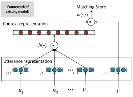
Figure 1

Existing models can be interpreted with a unified framework.f(·),f0(·),h(·), andm(·,·) are utterance representation function, response representation function, context representation function, and matching function, respectively.

a deep learning to respond architecture for multi-turn response selection; and Zhou et al. (2016) perform context-response matching from both a word view and an utterance view. Although these models are proposed from different backgrounds, we find that they can be interpreted with a unified framework, given by Figure 1. The framework consists of utterance representation f(·), response representation f0(·), context repre-sentationh(·), and matching calculationm(·,·). Given a contexts={u1,. . .,un}and a

response candidater,f(·) and f0(·) represent eachui in sandras vectors or matrices

byf(ui) and f0(r), respectively. {f(ui)}ni=1 are then uploaded to h(·), which transforms

the utterance representations intoh f(u1),. . .,f(un)

as a representation of the contexts. Finally,m(·,·) takesh f(u1),. . .,f(un)

andf0(r) as input and calculates a matching score forsandr. To sum up, the framework performs context-response matching following a paradigm that contextsand responserare first individually represented as vectors and then their matching degree is determined by the vectors. Under the framework, the matching modelg(s,r) can be defined withf(·),h(·),f0(·), andm(·,·), as follows:

g(s,r)=m h f(u1),. . .,f(un)

,f0(r)

(1)

The existing models are special cases under the framework with different defini-tions of f(·),h(·),f0(·), and m(·,·). Specifically, the RNN models in Lowe et al. (2015) can be defined as

mrnn(s,r)=σ

hrnn frnn(u1),. . .,frnn(un)

>

·M·f_rnn0 (r)+b (2)

where Mis a linear transformation, bis a bias, and σ(·) is a sigmoid function. ∀ui=

{wui,1,. . .,wui,ni},frnn(ui) is defined by

frnn(ui)=

~

wui,1,. . .,w~ui,k,. . .,w~ui,ni

wherew~ui,k is the embedding of thek-th wordwui,k, and [·] denotes a horizontal con-catenation operator on vectors or matrices.1 _{Suppose that the dimension of the word}

embedding is d, then the output of frnn(ui) is a d×ni matrix with each column an

embedding vector. Suppose thatr=(wr,1,. . .,wr,nr), thenf

0

rnn(r) is defined as

f_rnn0 (r)=RNN(w~r,1,. . .,w~r,k,. . .,w~r,nr) (4)

wherew~r,kis the embedding of thek-th word inr, and RNN(·) is either a vanilla RNN

(Elman 1990) or an RNN with LSTM units (Hochreiter and Schmidhuber 1997). RNN(·) takes a sequence of vectors as an input, and outputs the last hidden state of the network. Finally, the context representationhrnn(·) is defined by

hrnn frnn(u1),. . .,frnn(un)=RNN [frnn(u1),. . .,frnn(un)] (5)

In the deep learning to respond (DL2R) architecture (Yan, Song, and Wu 2016), the authors first transform the contextsto ans0={v1,. . .,vo}with heuristics

includ-ing “no context,” “whole context,” “add-one,” “drop-out,” and “combined.” These heuristics differ on how utterances before the last input in the context are incor-porated into matching. In “no context,” s0={un}, and thus no previous utterances

are considered; in “whole context,” s0={u1· · ·un,un} where operator glues

vectors together and forms a long vector. Therefore, in “whole context,” the conver-sation context is represented as a concatenation of all its utterances; in “add-one,”

s0={u1un,. . .,un−1un,un}. “add-one” leverages the conversation context by

con-catenating each of its utterances (except the last one) with the last input; in “drop-out,”

s0={(c\u1)un,. . ., (c\un−1)un,un}wherec=u1· · ·unandc\uimeans

exclud-inguifromc. “drop-out” also utilizes each utterance before the last one individually, but

concatenates the complement of each utterance with the last input; and in “combined,”

s0 is the union of the other heuristics. Let vo=un in all heuristics, then the matching

model of DL2R can be reformulated as

mdl2r(s,r)= o

X

i=1

MLP(fdl2r(vi)fdl2r(vo))·MLP(fdl2r(vi)fdl02r(r)) (6)

where MLP(·) is a multi-layer perceptron. ∀v∈ {v1,. . .,vo}, suppose that {w~v,1,. . .,

~

wv,nv}represent embedding vectors of the words inv, thenfdl2r(v) is given by

fdl2r(v)=CNN Bi-LSTM(w~v,1,. . .,w~v,nv)

(7)

where CNN(·) is a convolutional neural network (CNN) (Kim 2014) and Bi-LSTM(·) is a bi-directional recurrent neural network with LSTM units (Bi-LSTM) (Graves, Mohamed, and Hinton 2013). The output of Bi-LSTM(·) is all the hidden states of the Bi-LSTM model.f_dl0_2r(·) is defined in the same way withfdl2r(·). In DL2R, hdl2r(·) can be viewed

as an identity function on{fdl2r(v1),. . .,fdl2r(vo)}. Note that in the paper of Yan, Song,

and Wu (2016), the authors also assume that each response candidate is associated with an antecedent posting p. This assumption does not always hold in multi-turn

response selection. For example, in the Ubuntu Dialog Corpus (Lowe et al. 2015), there are no antecedent postings. To make the framework compatible with their assumption, we can simply extendfdl2r(r) to [fdl2r(p),fdl2r(r)], and definemdl2r(s,r) as

o X

i=1 

MLP(fdl2r(vi)fdl2r(vo))· 

 X

p

MLP(fdl2r(vi)fdl2r(p))·MLP(fdl2r(vi)fdl2r(r)) 

 

 (8)

Finally, in Zhou et al. (2016), the multi-view matching model can be rewritten as

mmv(s,r)=σ

hmv(fmv(u1),. . .,fmv(un))>

M1

M2

f_mv0 (r)+

b1

b2

(9)

where M1 and M2 are linear transformations, b1 and b2 are biases. ∀ui={wui,1,. . .,

wui,ni},fmv(ui) is defined as

fmv(ui)={fw(ui),fu(ui)} (10)

wherefw(ui) andfu(ui) are utterance representations from a word view and an utterance

view, respectively. The formulation offw(ui) andfu(ui) are given by

fw(ui)=

~

wui,1,. . .,w~ui,ni

fu(ui)=CNN(w~ui,1,. . .,w~ui,ni)

Suppose thatr=(wr,1,. . .,wr,nr), thenf

0

mv(r) is defined as

f_mv0 (r)=[f_w0(r)>,f_u0(r)>]> (11)

where the word view representation f_w0(r) and the utterance view representationf_u0(r) are formulated as

f_w0(r)=GRU(w~r,1,. . .,w~ur,nr)

f_u0(r)=CNN(w~r,1,. . .,w~ur,nr)

where GRU(·) is a recurrent neural network with GRUs (Cho et al. 2014). The out-put of fw0(r) is the last hidden state of the GRU model. The context representation

hmv(fmv(u1),. . .,fmv(un)) is defined as

hmv(fmv(u1),. . .,fmv(un))=[hw(fw(u1),. . .,fw(un))>,hu(fu(u1),. . .,fu(un))>]> (12)

where the word viewhw(·) and the utterance viewhu(·) are defined as

hw(fw(u1),. . .,fw(un))=GRU [fw(u1),. . .,fw(un)]

hu(fu(u1),. . .,fu(un))=GRU fu(u1),. . .,fu(un)

instinct connections among them. These models are nothing but similarity functions of a context representation and a response representation. Their difference on performance comes from how well the two representations capture the semantics and the structures of the context and the response and how accurate the similarity calculation is. For example, in empirical studies, the multi-view model performs much better than the RNN models. This is because the multi-view model captures the sequential relationship among words, the composition ofn-grams, and the sequential relationship of utterances byhw(·) and hu(·); whereas in RNN models, only the sequential relationship among

words are modeled byhrnn(·). Second, it is easy to make an extension of the existing

models by replacingf(·),f0(·),h(·), andm(·,·). For example, we can replace thehrnn(·)

in RNN models with a composition of CNN and RNN to model both composition of

n-grams and their sequential relationship, and we can replace themrnn(·) with a more

powerful neural tensor network (Socher et al. 2013). Third, the framework unveils the limitations the existing models and their possible extensions suffer: Everything in the context are compressed to one or more fixed-length vectors before matching; and there is no interaction between the context and the response in the formation of their repre-sentations. The context is represented without enough supervision from the response, and so is the response. As a result, these models may lose important information of contexts in matching, and more seriously, no matter how we improve them, as long as the improvement is under the framework, we cannot overcome the limitations. The framework view motivates us to propose a new framework that can essentially change the existing matching paradigm.

5. Sequential Matching Framework

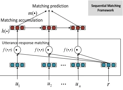
We propose a sequential matching framework (SMF) that can simultaneously capture important information in a context and model relationships among utterances in the context. Figure 2 gives the architecture of SMF. SMF consists of utterance–response matchingf(·,·), matching accumulation h(·), and matching prediction m(·). The three

1

u

u

r

Matching prediction Sequential Matching Framework

2 u ( )

h

( ) m Matching accumulation

( , )

f f( , ) f( , )

Utterance-response matching







Figure 2

components are organized in a three-layer architecture. Given a contexts={u1,. . .,un}

and a response candidater, the first layer matches eachuiinswithrthroughf(·,·) and

forms a sequence of matching vectors {f(u1,r),. . .,f(un,r)}. Here, we requiref(·,·) to

be capable of differentiating important parts from unimportant parts in ui and carry

the important information into f(ui,r). Details of how to design such a f(·,·) will be

described later. The matching vectors {f(u1,r),. . .,f(un,r)}are then uploaded to the

second layer whereh(·) models relationships and dependencies among the utterances

{u1,. . .un}. Here, we define h(·) as a recurrent neural network whose output is a

sequence of hidden states{h1,. . .,hn}.∀k∈ {1,. . .,n},hkis given by

hk=h0

hk−1,f(uk,r)

(13)

where h0(·,·) is a non-linear transformation, and h0=0. h(·) accumulates matching

vectors{f(u1,r),. . .,f(un,r)}in its hidden states. Finally, in the third layer, m(·) takes

{h1,. . .,hn}as an input and predicts a matching score for (s,r). In brief, SMF matchess

andrwith ag(s,r) defined as

g(s,r)=m

hf(u1,r),f(u2,r),. . .,f(unir)

(14)

SMF has two major differences over the existing framework: first, SMF lets each utterance in the context and the response “meet” at the very beginning, and therefore utterances and the response can sufficiently interact with each other. Through the inter-action, the response will help recognize important information in each utterance. The information is preserved in the matching vectors and carried into the final matching score with minimal loss; second, matching and utterance relationships are coupled rather than separately modeled as in the existing framework. Hence, the utterance relationships (e.g., the order of the utterances), as a kind of knowledge, can supervise the formation of the matching score. Because of the differences, SMF can overcome the drawbacks the existing models suffer and tackle the two challenges of context-response matching simultaneously.

It is obvious that the success of SMF lies in how to designf(·,·), becausef(·,·) plays a key role in capturing important information in a context. In the following sections, we will first specify the design off(·,·), and then discuss how to defineh(·) andm(·).

5.1 Utterance–Response Matching

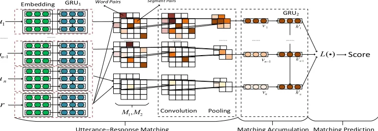
Figure 3

The architecture of SCN. The first layer extracts matching information from interactions between utterances and a response on a word level and a segment level by a CNN. The second layer accumulates the matching information from the first layer by a GRU. The third layer takes the hidden states of the second layer as an input and calculates a matching score.

5.1.1 Sequential Convolutional Network.Figure 3 gives the architecture of SCN. Given an utteranceuin a contextsand a response candidater, SCN looks up an embedding table and representsuandrasU=eu,1,. . .,eu,nu

andR=er,1,. . .,er,nr

, respectively, where

eu,i,er,i∈Rdare the embeddings of thei-th word ofuandr, respectively. WithUandR, SCN constructs a word–word similarity matrixM1 ∈Rnu×nr and a sequence–sequence similarity matrixM2∈Rnu×nras two input channels of a convolutional neural network (CNN). The CNN then extracts important matching information from the two matrices and encodes the information into a matching vectorv.

Specifically,∀i,j, the (i,j)-th element ofM1is defined by

e1,i,j=eu>,i·er,j (15)

M1models the interaction betweenuandron a word level.

To getM2, we first transformUandRto sequences of hidden vectors with a GRU.

Suppose that Hu=

hu,1,. . .,hu,nu

are the hidden vectors of U, then ∀i, hu,i∈Rm is defined by

zi=σ(Wzeu,i+Uzhu,i−1)

ri=σ(Wreu,i+Urhu,i−1)

eh_u,i=tanh(W_he_u,i+U_h(r_ih_u,i−1))

hu,i=zieh_u,i+(1−z_i)h_u,i−1 (16)

where hu,0=0, zi and ri are an update gate and a reset gate respectively, σ(·) is a

sigmoid function, and Wz, Wh, Wr, Uz, Ur,Uh are parameters. Similarly, we have

Hr=

hr,1,. . .,hr,nr

as the hidden vectors ofR. Then, ∀i,j, the (i,j)-th element ofM2

is defined by

whereA∈Rm×mis a linear transformation.∀i, GRU encodes the sequential information and the dependency among words until positioniinuinto thei-th hidden state. As a consequence,M2models the interaction betweenuandron a segment level.

M1 andM2are then processed by a CNN to compute the matching vectorv.∀f =

1, 2, CNN regardsMf as an input channel, and alternates convolution and max-pooling

operations. If we denote the k-th feature map at thel-th layer as zk_{, whose filters are}

determined by a tensorWkand a biasbk, then the feature mapzkis obtained as follows:

zk_i,j=σ((Wk∗z0)i,j+bk) (18)

zk_i,j=σ

X

u

Wu_k∗z0_u

i,j

+bk

(19)

where σ(·) is a ReLU,Wu_k is the weight of the u-th feature map, z0=(z0₁. . .z0_u. . .z0_U) is feature maps on the (l−1)-th layer, andUis the number of feature maps. Notably, ∗is a 2D convolutional operation, sliding a window on feature maps at that layer, that is formulated as

(W∗o)m,n= width

X

i=0 height

X

j=0

Wi,j·om+i,n+j (20)

wherewidthandheightare the hyper-parameters of the convolutional window, ando=

z0u . A max pooling operation follows a convolution operation and picks the maximal

values within a window sliding on the output of the convolution operation, and carries out a linear transformation on the feature values within the window. The max pooling operation can be formulated as

zk_i,j=maxz(i:i+pw,j:j+ph) (21)

where pw and ph are the width and the height of the 2D pooling, respectively. The

matching vector v is defined by concatenating outputs of the last feature maps and transforming it to a low dimensional space:

v=Wc[z0,z1. . .,zf

0

]+bc (22)

wheref0denotes the number of feature maps,Wcandbcare parameters, andzkis the

concatenation of elements at thek-th feature map, meaningzk_=[zk

0,0,zk0,1. . .zkI,J] where

IandJare the maximum indices of the feature map.

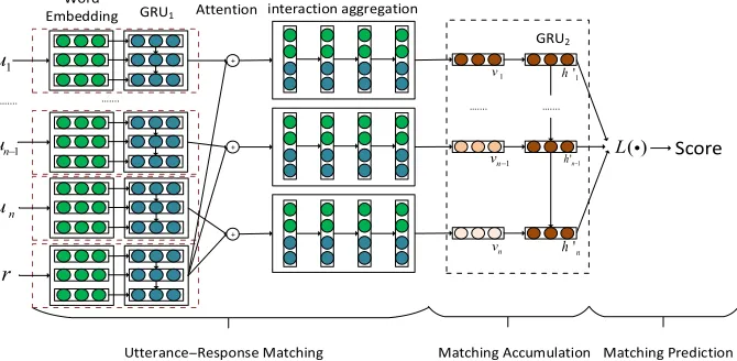
Figure 4

The architecture of SAN. The first layer highlights important words and segments in context, and computes a matching vector from both word level and segment level. Similar to SCN, the second layer uses a GRU to accumulate the matching information, and the third layer predicts the final matching score.

5.1.2 Sequential Attention Network.With word embeddingsUandRand hidden vectors Hu and Hr, SAN also performs utterance–response matching on a word level and a

segment level. Figure 4 gives the architecture of SAN. In each level of matching, SAN exploits every part of the response (either a word or a hidden state) to weight the parts of the utterance and obtain a weighted representation of the utterance. The utterance representation then interacts with the part of the response. The interactions are finally aggregated following the order of the parts in the response as a matching vector.

Specifically,∀er,i∈R, the weight ofeu,j∈Uis given by

ω_i,j=tanh(e>_u,jWatt1er,i+batt1) (23)

α_i,j= Pneuωi,j

j=1e

ωi,j (24)

whereWatt1∈Rd×d, andbatt1∈Rare parameters.ωi,j∈Rrepresents the importance of

eu,jin the utterance corresponding toer,iin the response.αi,jis normalized importance.

The interaction betweenuander,iis then defined as

t1,i=





nu

X

j=1

α_i,jeu,j



e_r,i (25)

where (Pnu

j=1αi,jeu,j) is the representation of u with weights {αi,j}nj=u1, and is the

Similarly,∀hr,i∈Hr, the weight ofhu,j∈Hucan be defined as

ω0_i,j=v0>tanh(h>_u,jWatt2hr,i+batt2) (26)

α0_i,j= e

ω0 i,j

Pnu

j=1e

ω0

i,j (27)

whereWatt2∈Rd×d,v0∈Rd, andbatt2∈Rd are parameters. The interaction betweenu

andhr,ithen can be formulated as

t2,i= nu

X

j=1

α0_i,jhu,j

hr,i (28)

We denote the attention weights {α_i,j} and {α_i0_,j} as A1 and A2, respectively. With

the word-level interaction T1=[t1,1,. . .,t1,nr] and the segment level interaction T2= [t2,1,. . .,t2,nr], we form aT=[t1,. . .,tnr] by definingtias [t

>

1,i,t>2,i]>. The matching vector

vof SAN is then obtained by processingTwith a GRU:

v=GRU(T) (29)

where the specific parameterization of GRU(·) is similar to Equation (16), and we take the last hidden state of the GRU asv.

From Equations (23) and (26), we can see that SAN identifies important information in utterances in a context through an attention mechanism. Words or segments in utterances that are useful to recognize the appropriateness between the context and a response will receive high weights from the response. The information conveyed by these words and segments will be highlighted in the interaction between the utterances and the response and carried to the matching vector through a RNN that models the aggregation of information in the utterances under the supervision of the response. Similar to SCN, we will further investigate the effect of the attention mechanism in SAN by visualizing the attention weights in Section 7.

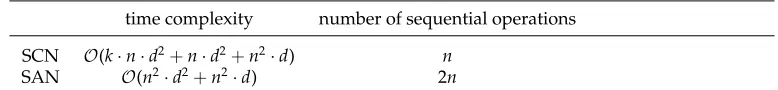
5.1.3 SAN vs. SCN.Because SCN and SAN exploits different mechanisms to understand important parts in contexts, an interesting question arises: What are the advantages and disadvantages of the two models in practice? Here, we leave empirical comparison of their performance to experiments and first compare SCN with SAN on the following aspects: (1) amount of parallelable computation, which is measured by the minimum number of sequential operations required; and (2) total time complexity.

Table 2 summarizes the comparison between the two models. In terms of parallel-ability, SAN uses two RNNs to learn the representations, which requires 2nsequential operations, whereas SCN has n sequentially executed operations in the construction ofM2. Hence, SCN is easier to parallelize than SAN. In terms of time complexity, the

complexity of SCN isO(k·n·d2+n·d2+n2·d), wherekis the number of feature maps in convolutions,nismax(nu,nr), anddis embedding size. More specifically, in SCN, the

cost on construction ofM1andM2isO(n·d2+n2·d), and the cost on convolution and

pooling isO(k·n·d2). The complexity of SAN isO(n2·d+n2·d2), whereO(n2·d) is the cost on calculatingHuandHrandO(n2·d2) is the cost of the following

Table 2

Comparison between SCN and SAN.kis the kernel number of convolutions.nismax(nu,nr).dis

the embedding size.

time complexity number of sequential operations

SCN O(k·n·d2_+n·d2_+n2_{·d) n}

SAN O(n2_·d2_+n2_{·d) 2n}

Therefore, SCN could be faster than SAN. The conclusion is also verified by empirical results in Section 7.

5.2 Matching Accumulation

The function of matching accumulation h(·) in SMF can be implemented with any recurrent neural networks such as LSTM and GRU. In this work, we fixh(·) as GRU in both SCN and SAN. Given{f(u1,r),. . .,f(un,r)}as the output of the first layer of

SMF, the non-linear transformationh0(·,·) in Equation (13) is formulated as

z0_i =σ(Wz0f(ui,r)+Uz0hi−1)

r0_i =σ(Wr0f(ui,r)+Ur0hi−1)

e

hi=tanh(Wh0f(ui,r)+Uh0(rih0i−1))

hi=zieh_i+(1−z_i)h_i−1 (30)

where Wz0, Wh0, Wr0, Uz0, Ur0,Uh0 are parameters, and z0i and r0i are an update gate

and a reset gate, respectively. Here,hi is a hidden state, which encodes the matching

information in its previous turns. From Equation (30) we can see that the reset gate (i.e.,

ri) and the update gate (i.e.,zi) control how much information from the current matching

vectorf(ui,r) flows into the accumulation vectorhi. Ideally, the two gates should let

matching vectors that correspond to important utterances make a great impact to the accumulation vectors (i.e., the hidden states) while blocking the information from the unimportant utterances. In practice, we find that we can achieve this by learning SCN and SAN from large-scale conversation data. The details will be given in Section 7.

5.3 Matching Prediction

m(·) takes{h1,. . .,hn}from h(·) as an input and predicts a matching score for (s,r).

We consider three approaches to implementingm(·).

5.3.1 Last State.The first approach is that we only use the last hidden statehnto calculate

a matching score. The underlying assumption is that important information in the context, after selection by the gates of the GRU, has been encoded into the vectorhn.

Thenm(·) is formulated as

mlast(h1,. . .,hn)=softmax(Wlhn+bl) (31)

5.3.2 Static Average.The second approach is combining all hidden states with weights determined by their positions. In this approach,m(·) can be formulated as

mstatic(h1,. . .,hn)=softmax(Ws(

n

X

i=1

wihi)+bs) (32)

where Ws andbs are parameters, andwi is the weight of thei-th hidden state and is

learned from data. Note that inmstatic(·), once{wi}ni=1are learned, they are fixed for any

(s,r) pairs, and that is why we call the approach “static average.” Compared with last state, the static average can leverage more information in the early parts of{h1,. . .,hn},

and thus can avoid information loss from the process of the GRU inh(·).

5.3.3 Dynamic Average. Similar to static average, we also combine all hidden states to calculate a matching score, but the difference is that the combination weights are dynamically computed by the hidden states and the utterance vectors through an attention mechanism as in Bahdanau, Cho, and Bengio (2014). The weights will change according to the content of the utterances in different contexts, and that is why we call the approach “dynamic average.” In this approach,m(·) is defined as

ti=t>s tanh(Wd1hu,nu+Wd2hi+bd1)

α_i= Pexp(ti)

iexp(ti)

m(h1,. . .,hn)=softmax(Wd( n

X

i=1

α_ihi)+bd2) (33)

whereWd1∈Rq×m,Wd2∈Rq×q,bd1∈Rq,Wd∈Rq×q, andbd2∈Rqare parameters.ts

is a virtual context vector that is learned in training.hiandhu,nuarei-th hidden state of

h(·) and the final hidden state of the utterance, respectively.

6. Model Training

We choose cross entropy as the loss function. LetΘdenote the parameters off(·,·),h(·,·), andm(·), then the objective functionL(D,Θ) can be written as

L(D,Θ)=−

N

X

i=1

yilog(g(si,ri))+(1−yi)log(1−g(si,ri))

(34)

7. Experiments

We test SAN and SCN on two public data sets with both quantitative metrics and qualitative analysis.

7.1 Data Sets

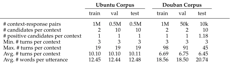
The first data set we exploited to test the performance of our models is the Ubuntu Dialogue Corpus v1 (Lowe et al. 2015). The corpus contains large-scale two-way conver-sations collected from the chat logs of the Ubuntu forum. The converconver-sations are multi-turn discussions about Ubuntu-related technical issues. We used the copy shared by Xu et al. (Xu et al. 2017),2 _{in which numbers, URLs, and paths are replaced by special}

placeholders. The data set consists of 1 million context-response pairs for training, 0.5 million pairs for validation, and 0.5 million pairs for testing. In each conversation, a human reply is selected as a positive response to the context, and negative responses are randomly sampled. The ratio of positive responses and negative responses is 1:1 in the training set, and 1:9 in both the validation and test sets.

In addition to the Ubuntu Dialogue Corpus, we selected the Douban Conversation Corpus (Wu et al. 2017) as another data set. The data set is a recently released large-scale open-domain conversation corpus in which conversations are crawled from a popular Chinese forum Douban Group.3 The training set contains 1 million context-response pairs, and the validation set contains 50, 000 pairs. In both sets, a context has a human reply as a positive response and a randomly sampled reply as a nega-tive response. Therefore, the ratio of posinega-tive instances and neganega-tive instances in both training and validation is 1:1. Different from the Ubuntu Dialogue Corpus, the test set of the Douban Conversation Corpus contains 1, 000 contexts with each one having 10 responses retrieved from a pre-built index. Each response receives three labels from human annotators that indicate its appropriateness as a reply to the context and the majority of the labels are taken as the final decision. An appropriate response means that the response can naturally reply to the conversation history by satisfying logic consistency, fluency, and semantic relevance. Otherwise, if a response does not meet any of the three conditions, it is an inappropriate response. The Fleiss kappa (Fleiss 1971) of the labeling is 0.41, which means that the labelers reached a moderate agreement in their work. Note that in our experiments, we removed contexts whose responses are all labeled as positive or negative. After this step, there are 6, 670 context-response pairs left in the test set.

Table 3 summarizes the statistics of the two data sets.

7.2 Baselines

We compared our methods with the following methods:

TF-IDF: We followed Lowe et al. (2015) and computed TF-IDF-based cosine simi-larity between a context and a response. Utterances in the context are concatenated to form a document. IDF is computed on the training data.

Basic deep learning models: We used models in Lowe et al. (2015) and Kadlec, Schmid, and Kleindienst (2015), in which representations of a context are learned by

Table 3

Statistics of the two data sets.

Ubuntu Corpus Douban Corpus

train val test train val test

# context-response pairs 1M 0.5M 0.5M 1M 50k 10k

# candidates per context 2 10 10 2 2 10

# positive candidates per context 1 1 1 1 1 1.18

Min. # turns per context 3 3 3 3 3 3

Max. # turns per context 19 19 19 98 91 45

Avg. # turns per context 10.10 10.10 10.11 6.69 6.75 6.45

Avg. # words per utterance 12.45 12.44 12.48 18.56 18.50 20.74

neural networks with the concatenation of utterances as inputs and the final matching score is computed by a bilinear function of the context representation and the response representation. Models including RNN, CNN, LSTM, and BiLSTM were selected as baselines.

Multi-View: The model proposed in Zhou et al. (2016) that utilizes a hierarchical recurrent neural network to model utterance relationships. It integrates information in a context from an utterance view and a word view. Details of the model can be found in Equation (9).

Deep learning to respond (DL2R): The authors in Yan, Song, and Wu (2016) pro-posed several approaches to reformulate a message with previous turns in a context. The response and the reformulated message are then represented by a composition of RNN and CNN. Finally, the matching score is computed with the concatenation of the representations. Details of the model can be found in Equation (6).

Advanced single-turn matching models: Because BiLSTM does not represent the state-of-the-art matching model, we concatenated the utterances in a context and matched the long text with a response candidate using more powerful models, includ-ing MV-LSTM (Wan et al. 2016b) (2D matchinclud-ing), Match-LSTM (Wang and Jiang 2016b), and Attentive-LSTM (Tan et al. 2016) (two attention based models). To demonstrate the importance of modeling utterance relationships, we also calculated a matching score for the concatenation of utterances and the response candidate using the methods in Section 5.1. The two models are simple versions of SCN and SAN, respectively, with-out considering utterance relationships. We denote them as SCNsingle and SANsingle,

respectively.

7.3 Evaluation Metrics

In experiments on the Ubuntu corpus, we followed Lowe et al. (2015) and used recall at positionkinncandidates (Rn@k) as evaluation metrics. Here the matching models are

required to returnkmost likely responses, andRn@k=1 if the true response is among

thekcandidates.Rn@kwill become larger whenkgets larger orngets smaller.

Rn@k has bias when there are multiple true candidates for a context. Hence, on

the Douban corpus, apart fromRn@ks, we also followed the convention of information

1999), mean reciprocal rank (MRR) (Voorhees and Tice 2000), and precision at position 1 (P@1) as evaluation metrics, which are defined as follows

MAP= 1

|S|

X

si∈S

AP(si) , where AP(si)=

PNr

j=0

Pj

k=0rel(rk,si)

j ·rel(rj,si)

PNr

j=0rel(rj,si)

(35)

MRR= 1

|S|

X

si∈S

RR(si) , where RR(si)= _rank1

i (36)

P@1= 1

|S|

X

si∈S

rel(rtop1,si) (37)

whererankirefers to the position of the first relevant response to contextsiin the ranking

list;rjrefers to the response ranked at thej-th position;rel(rj,si)=1 ifrjis an appropriate

response to contextsi, otherwiserel(rj,si)=0; rtop1 is the response ranked at the top

position;S is the universal set of contexts; and Nr denotes the number of retrieved

responses.

We did not calculate R2@1 for the test data in the Douban corpus because one

context could have more than one correct response, and we have to randomly sample one forR2@1, which may bring bias to the evaluation.

7.4 Parameter Tuning

For baseline models, we copied the numbers in the existing papers if their results on the Ubuntu corpus are reported in their original paper (TF-IDF, RNN, CNN, LSTM, BiLSTM, Multi-View); otherwise we implemented the models by tuning their parame-ters on the validation sets. All models were implemented using the Theano framework (Theano Development Team 2016). Word embeddings in neural networks were initial-ized by the results of word2vec (Mikolov et al. 20134_{) pre-trained on the training data.}

We did not use GloVe (Pennington, Socher, and Manning 2014) because the Ubuntu corpus contains many technical words that are not covered by Twitter or Wikipedia. The word embedding size was chosen as 200. The maximum utterance length was set as 50. The maximum context length (i.e., number of utterances per context) was varied from 1 to 20 and set as 10 at last. We padded zeros if the number of utterances in a context is less than 10; otherwise we kept the last 10 utterances. We will discuss how the performance of models changes in terms of different maximum context length later.

For SCN, the window size of convolution and pooling was tuned to {(2, 2), (3, 3)(4, 4)}and was set as (3, 3) finally. The number of feature maps is 8. The size of the hidden states in the construction ofM2is the same with the word embedding size,

and the size of the output vectorvwas set as 50. Furthermore, the size of the hidden states in the matching accumulation module is also 50. In SAN, the size of the hidden states in the segment level representation is 200, and the size of the hidden states in Equation (29) was set as 400.

All tuning was done according toR2@1 on the validation data.

7.5 Evaluation Results

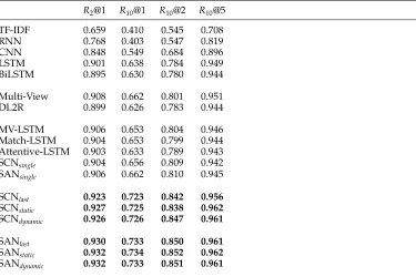
Tables 4 and 5 show the evaluation results on the Ubuntu Corpus and the Douban Corpus, respectively. SAN and SCN outperform baselines over all metrics on both data sets with large margins, and except for R10@5 of SCN on the Douban corpus,

the improvements are statistically significant (t-test with p-value≤0.01). Our models are better than state-of-the-art single turn matching models such as MV-LSTM, Match-LSTM, SCNsingle, and SANsingle. The results demonstrate that one cannot neglect

utter-ance relationships and simply perform multi-turn response selection by concatenating utterances together.

TF-IDF shows the worst performance, indicating that the multi-turn response selec-tion problem cannot be addressed with shallow features. LSTM is the best model among the basic models. The reason might be that it models relationships among words. Multi-View is better than LSTM, demonstrating the effectiveness of the utterance-view in context modeling. Advanced models have better performance, because they are capable of capturing more complicated structures in contexts.

SAN is better than SCN on both data sets, which might be attributed to three reasons. The first reason is that SAN uses vectors instead of scalars to represent in-teractions between words or text segments. Therefore, the matching vectors in SAN can encode more information from the pairs than those in SCN. The second reason is that SAN uses a soft attention mechanism to emphasize important words or segments

Table 4

Evaluation results on the Ubuntu corpus. Subscripts including last, static, and dynamic indicate three approaches to predicting a matching score as described in Section 5.3. Numbers inbold

mean that the improvement from the models is statistically significant over the best baseline method.

R2@1 R10@1 R10@2 R10@5

TF-IDF 0.659 0.410 0.545 0.708

RNN 0.768 0.403 0.547 0.819

CNN 0.848 0.549 0.684 0.896

LSTM 0.901 0.638 0.784 0.949

BiLSTM 0.895 0.630 0.780 0.944

Multi-View 0.908 0.662 0.801 0.951

DL2R 0.899 0.626 0.783 0.944

MV-LSTM 0.906 0.653 0.804 0.946

Match-LSTM 0.904 0.653 0.799 0.944

Attentive-LSTM 0.903 0.633 0.789 0.943

SCNsingle 0.904 0.656 0.809 0.942

SANsingle 0.906 0.662 0.810 0.945

SCNlast 0.923 0.723 0.842 0.956

SCNstatic 0.927 0.725 0.838 0.962

SCNdynamic 0.926 0.726 0.847 0.961

SANlast 0.930 0.733 0.850 0.961

SANstatic 0.932 0.734 0.852 0.962

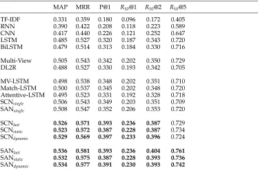
Table 5

Evaluation results on the Douban corpus. Notations have the same meaning as those in Table 4. OnR10@5, only SAN significantly outperforms baseline methods.

MAP MRR P@1 R10@1 R10@2 R10@5

TF-IDF 0.331 0.359 0.180 0.096 0.172 0.405

RNN 0.390 0.422 0.208 0.118 0.223 0.589

CNN 0.417 0.440 0.226 0.121 0.252 0.647

LSTM 0.485 0.527 0.320 0.187 0.343 0.720

BiLSTM 0.479 0.514 0.313 0.184 0.330 0.716

Multi-View 0.505 0.543 0.342 0.202 0.350 0.729

DL2R 0.488 0.527 0.330 0.193 0.342 0.705

MV-LSTM 0.498 0.538 0.348 0.202 0.351 0.710

Match-LSTM 0.500 0.537 0.345 0.202 0.348 0.720

Attentive-LSTM 0.495 0.523 0.331 0.192 0.328 0.718

SCNsingle 0.506 0.543 0.349 0.203 0.351 0.709

SANsingle 0.508 0.547 0.352 0.206 0.353 0.720

SCNlast 0.526 0.571 0.393 0.236 0.387 0.729

SCNstatic 0.523 0.572 0.387 0.228 0.387 0.734

SCNdynamic 0.529 0.569 0.397 0.233 0.396 0.724

SANlast 0.536 0.581 0.393 0.236 0.404 0.761

SANstatic 0.532 0.575 0.387 0.228 0.393 0.736

SANdynamic 0.534 0.577 0.391 0.230 0.393 0.742

in utterances, whereas SCN uses a max pooling operation to select important infor-mation from similarity matrices. When multiple words or segments are important in an utterance–response pair, a max pooling operation just selects the top one, but the attention mechanism can leverage all of them. The last reason is that SAN models the sequential relationship and dependency among words or segments in the interaction aggregation module, whereas SCN only considersn-grams.

The three approaches to matching prediction do not show much difference in both SCN and SAN, but dynamic average and static average are better than the last state on the Ubuntu corpus and worse than it on the Douban corpus. This is because contexts in the Ubuntu corpus are longer than those in the Douban corpus (average context length 10.1 vs. 6.7), and thus the last hidden state may lose information in history on the Ubuntu data. In contrast, the Douban corpus has shorter contexts but longer utterances (average utterance length 18.5 vs. 12.4), and thus noise may be involved in response selection if more hidden states are taken into consideration.

There are two reasons that Rn@ks on the Douban corpus are much smaller than

those on the Ubuntu corpus. One is that response candidates in the Douban corpus are returned by a search engine rather than negative sampling. Therefore, some negative responses in the Douban corpus might be semantically closer to the true positive re-sponses than those in the Ubuntu corpus, and thus more difficult to differentiate by a model. The other is that there are multiple correct candidates for a context, so the maximumR10@1 for some contexts are not 1. For example, if there are three correct

responses, then the maximumR10@1 is 0.33. P@1 is about 40% on the Douban corpus,

7.6 Further Analysis

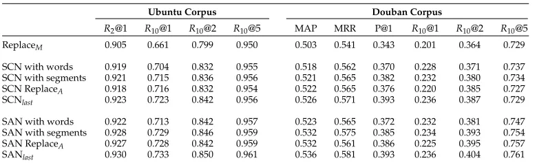
7.6.1 Model Ablation. We first investigated how different parts of SCN and SAN affect their performance by ablating SCNlastand SANlast. Table 6 reports the results of ablation

on the test data. First, we replaced the utterance–response matching module in SCN and SAN with a neural tensor (Socher et al. 2013) (denoted as ReplaceM), which matches an

utterance and a response by feeding their representations to a neural tensor network (NTN). The result is that the performance of the two models dropped dramatically. This is because in NTN there is no interaction between the utterance and the response before their matching; and it is doubtful whether NTN can recognize important parts in the pair and encode the information into matching. As a result, the model loses important information in the pair. Therefore, we can conclude that a good utterance–response matching mechanism is crucial to the success of SMF. At least, one has to let an utterance and a response interact with each other and explicitly highlight important parts in their matching vector. Second, we replaced the GRU in the matching accumulation modules of SCN and SAN with a multi-layer perceptron (denoted as SCN ReplaceA and SAN

ReplaceA, respectively). The change led to a slight performance drop. This indicates

that utterance relationships are useful in context-response matching. Finally, we only left one level of granularity, either word level or segment level, in SCN and SAN, and denoted the models as SCN with words, SCN with segments, SAN with words, and SAN with segments, respectively. The results indicate that segment level matching on utterance–response pairs contributes more to the final context-response matching, and both segments and words are useful in response selection.

7.6.2 Comparison with Respect to Context Length.We then studied how the performance of SCNlastand SANlastchanges across contexts with different lengths. Context-response

pairs were bucketed into three bins according to the length of the contexts (i.e., the number of utterances in the contexts), and comparison was made in different bins on different metrics. Figure 5 gives the results. Note that we did the analysis only on the Douban corpus because on the Ubuntu corpus many results were copied from the existing literatures and the bin-level results are not available. SAN and SCN consistently perform better than the baselines over bins, and a general trend is that when contexts become longer, gaps become larger. For example, in (2, 5], SAN is 3 points higher than LSTM onR10@5, but the gap becomes 5 points in (5, 10]. The results demonstrate that our

models can well capture dependencies, especially long-distance dependencies, among utterances in contexts. SAN and SCN have similar trends because both of them use a

Table 6

Evaluation results of model ablation.

Ubuntu Corpus Douban Corpus

R2@1 R10@1 R10@2 R10@5 MAP MRR P@1 R10@1 R10@2 R10@5

ReplaceM 0.905 0.661 0.799 0.950 0.503 0.541 0.343 0.201 0.364 0.729

SCN with words 0.919 0.704 0.832 0.955 0.518 0.562 0.370 0.228 0.371 0.737

SCN with segments 0.921 0.715 0.836 0.956 0.521 0.565 0.382 0.232 0.380 0.734

SCN ReplaceA 0.918 0.716 0.832 0.954 0.522 0.565 0.376 0.220 0.385 0.727

SCNlast 0.923 0.723 0.842 0.956 0.526 0.571 0.393 0.236 0.387 0.729

SAN with words 0.922 0.713 0.842 0.957 0.523 0.565 0.372 0.232 0.381 0.747

SAN with segments 0.928 0.729 0.846 0.959 0.532 0.575 0.385 0.234 0.393 0.754

SAN ReplaceA 0.927 0.728 0.842 0.959 0.532 0.561 0.386 0.225 0.395 0.757

(2,5] (5,10] (10,)

context length

30

40

50

P@1

LSTM MV-LSTM Multi-View SCN SAN

(2,5] (5,10] (10,)

context length

40

45

50

55

60

MAP

LSTM MV-LSTM Multi-View SCN SAN

(2,5] (5,10] (10,)

context length

50

60

70

MRR

LSTM MV-LSTM Multi-View SCN SAN

(2,5] (5,10] (10,)

context length

15

20

25

30

R_10@1

LSTM MV-LSTM Multi-View SCN SAN

(2,5] (5,10] (10,)

context length

30

35

40

45

R_10@2

LSTM MV-LSTM Multi-View SCN SAN

(2,5] (5,10] (10,)

context length

65

70

75

80

R_10@5

LSTM MV-LSTM Multi-View SCN SAN

Figure 5

Model performance across context length. We compared SAN and SCN with LSTM, MV-LSTM, and Multi-View on the Douban corpus.

GRU in the second layer to model dependencies among utterances. The performance of all models drops when the length of contexts increases from (2, 5] to (5, 10]. This is because semantics of longer contexts is more difficult to capture than that of shorter contexts. On the other hand, the performance of all models improved when the length of contexts increases from (5, 10] to (10, ). This is because the bin of (10, ) contains much less data than the other two bins (the data distribution is 53% for (2, 5], 38% for (5, 10], and 9% for (10, )), and thus the improvement does not make much sense from a statistical perspective.

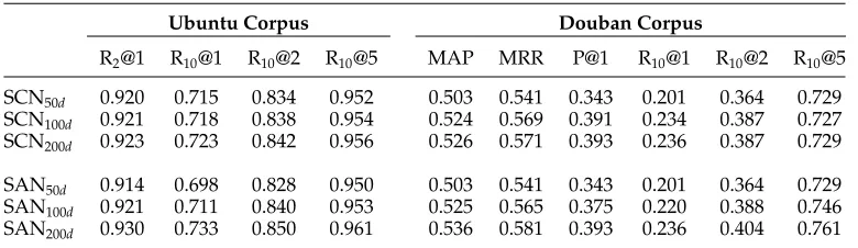
7.6.3 Sensitivity to Hyper-Parameters.We checked how sensitive SCN and SAN are re-garding the size of word embedding and the maximum context length. Table 7 reports evaluation results of SCNlastand SANlastwith embedding sizes varying in{50, 100, 200}.

Table 7

Evaluation results in terms of different word embedding sizes.

Ubuntu Corpus Douban Corpus

R2@1 R10@1 R10@2 R10@5 MAP MRR P@1 R10@1 R10@2 R10@5

SCN50d 0.920 0.715 0.834 0.952 0.503 0.541 0.343 0.201 0.364 0.729

SCN100d 0.921 0.718 0.838 0.954 0.524 0.569 0.391 0.234 0.387 0.727

SCN200d 0.923 0.723 0.842 0.956 0.526 0.571 0.393 0.236 0.387 0.729

SAN50d 0.914 0.698 0.828 0.950 0.503 0.541 0.343 0.201 0.364 0.729

SAN100d 0.921 0.711 0.840 0.953 0.525 0.565 0.375 0.220 0.388 0.746

We can see that SAN is more sensitive to the word embedding size than SCN. SCN becomes stable after the embedding size exceeds 100, whereas SAN keeps improving with the increase of the embedding size. Our explanation of the phenomenon is that SCN transforms word vectors and hidden vectors of GRU to scalars in the similarity matrices by dot products, thus information in extra dimensions (e.g., entries with indices larger than 100) might be lost; on the other hand, SAN leverages the whole

d-dimensional vectors in matching, so the information in the embedding can be ex-ploited more sufficiently.

Figure 6 shows the performance of SCN and SAN with respect to the maximum context length. We find that both models significantly become better with the increase of maximum context length when it is lower than 5, and become stable after the maximum context length reaches 10. The results indicate that utterances from early history can provide useful information to response selection. Moreover, model performance is more sensitive to the maximum context length on the Ubuntu corpus than it is on the Douban

1 2 3 4 5 6 7 8 9 10 11 12 13 14 15

Maximum context length

0.5 0.6 0.7 0.8 0.9

Score

Ubuntu Corpus

R2_1 R10_1 R10_2 R10_5

1 2 3 4 5 6 7 8 9 10 11 12 13 14 15

Maximum context length

0.35 0.40 0.45 0.50 0.55

Score

Douban Corpus

MAP MRR P_1

(a) Performance of SCN across different context lengths.

1 2 3 4 5 6 7 8 9 10 11 12 13 14 15

Maximum context length

0.5 0.6 0.7 0.8 0.9

Score

Ubuntu Corpus

R2_1 R10_1 R10_2 R10_5

1 2 3 4 5 6 7 8 9 10 11 12 13 14 15

Maximum context length

0.35 0.40 0.45 0.50 0.55 0.60

Score

Douban Corpus

MAP MRR P_1

(b) Performance of SAN across different context lengths.

Figure 6

Figure 7

Efficiency of SCN and SAN. The left panel shows the training time per batch with 200 dimensional word embeddings, and the right panel shows the inference time per batch. One batch contains 200 instances.

corpus. This is because utterances in the Douban corpus are longer than those in the Ubuntu corpus (average length 18.5 vs. 12.4), which means single utterances in the Douban corpus could contain more information than those in the Ubuntu corpus. In practice, we set the maximum context length to 10 to balance effectiveness and efficiency.

7.6.4 Model Efficiency.In Section 5.1.3, we theoretically analyzed the efficiency of SCN and SAN. To verify the theoretical results, we further empirically compared their effi-ciency using the training data and the test data of the two data sets. The experiments were conducted using Theano on a Tesla K80 GPU with a Windows Server 2012 oper-ation system. The parameters of the two models are described in Section 7.4. Figure 7 gives the training time and the test time of SAN and SCN. We can see that SCN is twice as fast as SAN in the training process (as a result of low time complexity and ease of parallelization), and saves 3 msec per batch in the test process. Moreover, different matching functions do not influence the running time as much, because the bottleneck is the utterance representation learning.

The empirical results are consistent with our theoretical results: SCN is faster than SAN. The results indicate that SCN is suitable for systems that care more about effi-ciency, whereas SAN can reach a higher accuracy with a little sacrifice of efficiency.

7.6.5 Visualization.We finally explained how SAN and SCN understand the semantics of conversation contexts by visualizing the similarity matrices of SCN, the attention weights of SAN, and the update gate and the reset gate of the accumulation GRU of the two models using an example from the Ubuntu corpus. Table 8 shows an example that is selected from the test set of the Ubuntu corpus and ranked at the top position by both SAN and SCN.

Figure 8(a) illustrates word–word similarity matrices M1 in SCN. We can see that

important words inu1such as “unzip,” “rar,” and “files” are recognized and highlighted

by words like “command,” “extract,” and “directory” inr. On the other hand, the simi-larity matrix ofrandu3is almost blank, as there is no important information conveyed

byu3. Figure 8(b) shows the sequence-to-sequence similarity matricesM2 in SCN. We

Table 8

An example for visualization from the Ubuntu corpus.

Context

u1: how can unzip many rar files at once?

u2: sure you can do that in bash

u3: okay how?

u4: are the files all in the same directory?

u5: yes they all are;

Response

Response: then the command glebihan should extract them all from/to that directory

also provide complementary matching information to M1. Figure 8(c) visualizes the

reset gate and the update gate of the accumulation GRU, respectively. Higher values in the update gate represent more information from the corresponding matching vector flowing into matching accumulation. From Figure 8(c), we can see thatu1 is crucial to

response selection and nearly all information from u1 and rflows to the hidden state

of GRU, whereas other utterances are less informative and the corresponding gates are almost “closed” to keep the information fromu1andruntil the final state.

Regarding SAN, Figure 9(a) and Figure 9(b) illustrate the word level attention weightsA1and segment level attention weightsA2, respectively. Similar to SCN,

impor-tant words such as “zip” and “file” and imporimpor-tant segments like “unzip many rar” get high weights, whereas function words like “that” and “for” are less attended. It should be