Financial Crisis Management in Emerging Countries: Optimal Level of International Reserves and Ex Ante Conditions for an International Lender of Last Resort Intervention

Munich Personal RePEc Archive

Financial Crisis Management in

Emerging Countries: Optimal Level of

International Reserves and Ex Ante

Conditions for an International Lender of

Last Resort Intervention

Ben Hassine Khalladi, hela

INSAT

2015

Online at

https://mpra.ub.uni-muenchen.de/96151/

1

Financial Crisis Management in Emerging Countries:

Optimal Level of International Reserves and

Ex Ante

Conditions for an International Lender of Last Resort

Intervention

Hela BEN HASSINE KHALLADI

Assistant Professor

National Institute of Applied Sciences and Technology (INSAT), University of Carthage

Centre Urbain Nord BP 676 - 1080 Tunis Cedex, Tunis 1080

Email: Hela.Khalladi@isgs.rnu.tn

Telephone number: (216) 22537012

2

Abstract:

In this paper, we approach financial crises from two different aspects: Prevention

and Management. Prevention from crises, here sudden stops, will be carried out

through international reserves accumulation (Jeanne & Rancière model, 2006).

The section of crises management will be undertaken by an International Lender

of last Resort (ILOLR), here the International Monetary Fund (IMF). Our study

shows that under an optimal level of international reserves, countries should resort

to international lending, but the efficiency of this latter depends on countries’

eligibility,

i.e

their external, budget and financial sustainability.

JEL :

F32, F34, F35, G01

3

1-Introduction

Over the last decades, we have noticed a significant recovery of international reserves held by emerging markets, especially in Asia. This has raised the issue of the optimal level of international reserves in emerging markets. However, the setting of this level needs a normative reference. In this paper, we have used the model developed by Jeanne & Rancière in 2006. This reserves’ accumulation represents an efficient way for emerging markets to face financial crisis, especially sudden stops. But if the country becomes aware that the reserves held are less than their optimal level, national authorities have to counterbalance this lack and find sources of international reserves. One of these sources is the International Lending of Last Resort, a role played nowadays by the International Monetary Fund (IMF).

So once the optimal level of reserves assessed, it becomes relevant to imagine the scenario in which this level is higher than the one really held by the country’s central bank. In this case, the higher crisis’ probability calls for the intervention of an International Lender Of Last Resort (ILOLR), i.e the International Monetary Fund (IMF). According to recent literature, the efficiency of this intervention is closely related to some ex ante conditions. At this stage, one should assess countries’ sustainability, especially key sectors of ex ante conditionality: external, fiscal and financial, in order to determine if the country is eligible or not to a potential credit line of the IMF. This evaluation will allow us to set efficiency conditions of an ILOLR thanks to an innovative method: Classification And Regression Tree (CART).

In this paper, we will first present a model of optimal reserves. Accumulation of exchange reserves represents in fact the “solution of first resort” against financial crises (Crises prevention). If country’s reserves decrease under its optimal level, authorities have to look for an international loan of last resort. The efficiency of such loans depends on the country’s external, fiscal and financial sustainability. An assessment of this latter is conducted in the second part of this paper using a non- parametric methodology (Classification and Regression Tree).

2- Literature Review:

4 (1996), IMF (1953, 2000), De Beaufort and Wijnholds (1977, 2001), Jeanne and Rancière (2006), Jeanne (2007), Kim (2008)... But the litterature before the 90’s was totally defined in terms of trade, mainly imports. This litterature was criticized especialy beacuse of the lack of a guideline of th eoptimal level of reserves for a country.

The notion of « reserves adequacy » has changed with the occurrence of the financial crises of the 90’s (Calvo 1996, Frankel et Rose, 1996 ; Sachs, Tornell et Velasco, 1996). These crises have triggered the need of holding reserves adequacy ratios in order to include the vulnerability of emerging countries’ balance of payments (IMF, 2000 and 2001 ; Bussière and Mulder, 1999 ; Mulder, 2000, Jeanne (2007), Chang and Velasco, 2001, Aizenman and Lee, 2005, Krugman, 1979 ; Flood and Garber, 1984, Detragiache and Spilimbergo, 2001). More recent papers have tried to assess the optimal level of reserves for emerging countries with a high sudden stops risk (Aizenman and Lee, 2005 ; Caballero and Panageas, 2004 ; Garcia and Soto, 2004)

In general, the literature adopted two alternative ways to assess the optimal level of reserves for a country. The first uses reserves adequacy indicators : Rodrik and Velasco (1999), Bussière and Mulder (1999) , Willett and al. (2004), Greenspan (1999), De Beaufort Wijnholds and Kapteyn (2001), Soto and al. (2004), De Beaufort Wijnholds and Kapteyn (2001), Kim and al. (2005), Shcherbakov (2002), Redrado and al. (2006), Li and Rajan (2005), Skala, Thimann and Wölfinger (2007), Beck and Rahbari (2008). The second way uses econometries techniques, usually called « optimal reserves analysis » because they assume that the level of reserves should be proportional to the optimal level plus an error term non correlated with the other explaining (Aizenman et Marion, 2003)

According to Jeanne & Rancière (2006), few studies have tried to quantify the level of reserves that a country has to hold to face balance of payment’s chocks. The model of optimal exchange reserves developed by Jeanne & Rancière (2006) has tried to overcome this insufficiency.

The authors explained that political authorities have often used rules with quantitative thresholds, because of lack of an appropriate normative quantitative framework. The most common used rule is the maintenance of a level of reserves equivalent to three months of imports. A more recent rule, “Greenspan- Guidotti” rule, consists in holding reserves that totally cover the external short term debt.

5 years during which most of countries faced financial turmoils due to the 2008 international financial crisis. Thus, our results will be compared to Jeanne & Rancière ones to see the impact of the recent crisis. As the authors, first, the probability of crises, one of useful variables of the model, will be computed as an unconditional probability. Then, this probability will be estimated on the basis of several fundamentals.

According to Guidotti & al. (2004), Jeanne & Rancière identify a sudden stop for the year t if the ratio of capital inflows in relation to GDP, kt = KAt/Yt , falls than more than 5% of

the GDP in relation to the previous year, i.e

k

< k

– 5%.

Starting from this point, we have tried to detect episodes of sudden stops for 41 emerging and developing countries on the period 1975- 2012. Seeing that data are annual, we could get the more recent values, thanks essentially to online databases like the World Economic Outlook of the IMF, while data ends in 2003 for Jeanne & Rancière. Our results are presented in the table of Appendix 1.

Jeanne & Rancière have considered a little opened country which could face a sudden stop of capital inflows. The country holds reserves in order to smooth the sudden stop impact on domestic absorption. The authors have first presented the main hypotheses of their model and derived than a closed expression of reserves optimal level.

The authors showed that the optimal level of reserves in normal times is a fixed fraction of output level:

R

= ρ Y

The optimal ratio of reserves in relation to output ρ is given by the following expression:

ρ = λ + γ -

[ 1-

λ – (δ+π)(λ+γ)]

Equation (1) represents the formula of optimal level of reserves according to Jeanne & Rancière model. Where :

- π : The non conditional sudden stop probability (number of years of crisis/ Total number of years);

- γ : The ratio of output loss (difference between growth rates during calm and crisis periods);

6 - r : The reserves return (average of US 3-month T-bills of the last 10 years;

- δ : The term premium (difference between T-Bonds and Fed Funds rates); - σ : The risk aversion;

- g: The real GDP growth.

3-

Methodology and data: Application of Jeanne & Rancière Model for

the period 1975- 2012:

As Jeanne & Rancière, we have tried to calibrate the model using the same sample of sudden stops obtained in the previous section. To do this, we have built a benchmark calibration on the basis of the sudden stop average of our sample.

Definitions of all parameters as well as data sources are given in the appendix 2. The results of our benchmark calibration are summarized in the table below:

Table 1. Results of benchmark calibration of the 7 parameters

Parameter Values Interval of changes

π Non- conditional crisis probability 0.24 [0,0.55]

λ Sudden Stop size 0.14 [0.06,0.54]

r Return of reserves 0.033 [0,0.19]

δ Term premium 0.015 [-0.025,0.035]

g Average of real GDP growth 0.045 [0.012,0.093]

σ Risk aversion 2 [1,10]

ϒ Output loss 0.041 [0,0.19]

Parameters π, λ and γ have been calibrated using arithmetic averages of our sample (cf. previous section) for the period 1975- 2012.

The parameter λ has been calibrated as the average level of (kt-1- kt) of our sample, i.e

the sudden stop size. This parameter reaches hence 14% per year in average.

7 those related to the international financial crisis of 2007- 2008. The period studied by Jeanne & Rancière ends in 2003.

The output cost γ has also been calibrated using the difference average between GDP growth rate in normal times and GDP growth rate really observed during the sudden stop. We have noticed that the growth rate declines by 2.6% in average following a sudden stop, and by 1.7% during the year following the sudden stop. We have hence set the parameter γ at 4.3% in our benchmark calibration.

The short term non-risky rate r is set at 3.3%. It consists in the average of US 3-months Treasury bills of the last ten years of the studied period, i.e between 2002 and 2012.

The term premium δ is the average difference between US 10-years Treasury bonds and the federal fund rate. According to this definition, the parameter δ is set up at 1.5.

The GDP growth g reaches 4.5% for our sample (out of crises periods). Finally, the risk aversion is set up at 2%, i.e its standard value in the literature related to growth and business cycles (Jeanne & Rancière, 2006).

Using the formula developed by Jeanne & Rancière (equation 1) for our sample of countries during the period 1975- 2008, the optimal level of reserves is set up at 13,5% of GDP. Certainly, this level is close to the observed level of our sample between 1975 and 2012 (12%), but it is highly lower than the one observed during the more recent period 2000- 2012, when it reached 18% of the GDP in average. This goes in line with our starting idea: Emerging markets tend to accumulate too much exchange reserves in relation to their needs. Even accumulation seems to be understandable seeing the financial crises that hit emerging markets during the late 90’s, but this abundance can create costs.

Now, we will reckon once again the optimal level of exchange reserves of the same countries, replacing the non-conditional crises probability, π, by a probability that we will estimate thanks to a Probit model.

First, we will assess an empirical equation for the sudden stop probability π, based on a set of countries’ fundamentals and a Probit model.

Here, the probability of a sudden stop depends on countries’ economics fundamentals. It consists in a Probit Model of our 41 countries sample, between 1975 and 2012.

8 1- Debt variables: short term debt and public debt (related to GDP);

2- Exchange variables: real exchange rate over- valuation and exchange regimes; 3- Financial variables: US interest rates and their changes, financial openness (capital

inflows, total of capital inflows and outflows, foreign direct investments, external liabilities and Net Foreign Assets); country’s financial development (bank deposits, M2 and M2 multiplier, M3, stock exchange capitalization and credits to private sector);

4- Variables related to external trade (trade openness, terms of trade); 5- Variables of economic cycle: Real GDP growth and real credit growth.

We have collected 23 potential variables (cf. Appendix 2). All explaining variables have been delayed by one year. Then, we have eliminated the less significant variables from our estimation (general to specific approach, see Jeanne & Rancière, 2006). Our results are summarized in the Table 2. It appears that the sudden stop probability decreases with national GDP and the sum of capital inflows and outflows. This probability increases with capital inflows.

Table 2. Probit estimation of Sudden Stops crises

Variable Coefficient Std. Err. Z Proba.

Capital Inflows 8.955 1.854 4.83 0.000*

Capital Inflows and Outflows -4.550 1.057 -4.30 0.000*

Real GDP Growth -2.010 1.204 -1.67 0.095**

Constant -0.907 0.127 -7.13 0.000*

Sources: International Financial Statistics, IMF * : Significant at 5% ; ** : Significant at 10%

These results are consistent with the crises theory. A sustainable economic growth helps countries facing sudden stops crises. This situation reflects in fact country’s sound situation. For foreign investors, this reflects the ability of the country to face potential contagion. The resistance of the major emerging countries, like China, India or Brazil with their substantial annual growth rates during 2008 international financial crisis, is a perfect example for this idea.

9 is negative. The impact of financial integration degree on crises occurrence appears consequently unclear. The effect depends on the quality and the duration of foreign capitals, which determines in fine the vulnerability degree of a country facing a potential situation reversal.

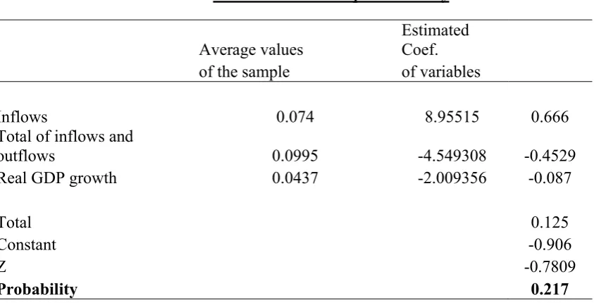
As Jeanne & Rancière, we have assessed the impact of fundamentals’ change on the optimal level of reserves of our “reference country”. To do this, our benchmark economy is calibrated as an average intermediate- level country, whose fundamentals are initially set up at the sample average.

Table 3. Sudden Stop Probability

Average values Estimated Coef.

of the sample of variables

Inflows 0.074 8.95515 0.666

Total of inflows and

outflows 0.0995 -4.549308 -0.4529

Real GDP growth 0.0437 -2.009356 -0.087

Total 0.125

Constant -0.906

Z -0.7809

Probability 0.217

where Z = 8.9551 * (Average of « Capital inflows ») – 4.5493 * (Average of « Capital Inflows and Outflows » ) -2.0093 * (Average of Real GDP Growth ) – 0.9067

The Probit data gives a sudden stop probability of 22% for our average economy, versus 24% in the case of non- conditional probability. When applying Jeanne & Rancière formula 1, this probability gives a ratio of 13.3% of optimal reserves in relation to GDP.

Then, we have analyzed the effect of a change in each significant variable (or fundamental) on the estimated probability of a sudden stop, and consequently on the optimal ratio of reserves.

10

Table 4. Marginal Impact of significant variables on a the Sudden stop probability

Variable dF/dx Std. Err. Z Proba.

Capital Inflows 2,6604 0,8123 3,26 0,001

Capital Inflows and Outflows -1,3411 0,4335 -3,08 0,002

Real GDP Growth -0,8438 0,3307 -2,54 0,011

According to the first colon of table 4, the probability of crises seems to be highly sensitive vis-a-vis variables changes. Hence, a slight increase of 1% in GDP growth reduces the crisis probability by 84%. Variables related to international financial integration are even more sensitive: a rise of 1% in capital inflows increases sharply the crisis risk (by 266%), while the same rise in capital inflows and outflows decreases this probability by 134%.

We should notice that these estimations are related to an average, in other words to an imaginary economy. It would be highly interesting to study a particular country, especially the impact of its fundamentals’ changes on the probability of crises.

Holding important international reserves represents indeed the solution of first resort when a country faces a crisis. The recourse to the IMF, considered as a solution of last resort, is considered when a country faces a hardening of its exchange reserves (lower than the optimal one).

Financial Crisis’ Management : Optimality conditions for a Bailout

from an International Lender of Last Resort :

11

4-1 Using CART methodology for the determination of external, fiscal and financial vulnerability thresholds :

We use data of 41 emerging countries for the period 1975- 2012. We get the debt crisis indicator from data provided by Standard and Poor’s as well as IMF lending Arrangements. A country is defined to be in debt crisis if it is classified as being in default by Standard and Poor’s, or if it has access to non concessional IMF financing in excess of 100% of quota (Manasse, Roubini and Schimmelpfennig, 2003). We used the definition of debt crisis because it represents the insolvency of a country that we have to distinguish from the illiquidity one. The intervention of the ILOR is in fact effective only in case of liquidity problems.

According to Standard and Poor’s, a country is defined to be in default if the government fails to pay the principal and the interests of external bonds on due date. The problem with this definition is that it may not capture “quasi- defaults”, i.e cases when defaults were prevented thanks to an adjustment program and a large financial package from the IMF (Manasse, Roubini and Schimmelpfennig, 2003). We therefore complete information with data on IMF non concessional lending from the IMF’s Finance Department1. Information collected is mainly related to loans approved, approval dates and the actual disbursements of the loans.

Hence, our definition of a debt crisis includes actual defaults on debts, recorded by Standard and Poor’s as well as defaults that were prevented through a “substantial” financial support from the IMF. For Manasse & al., an IMF “substantial” loan is the one exceeding 100% of the country’s quota. According to this definition, sixty- five (65) crisis episodes were identified:

12

Table 5- Debt Crises Episodes 1975- 2012

Pays Nombre de crises Nombre d'années en crise Episodes de crises (Entrée- Sortie)

Argentina 3 20 1982-1994; 1995- 1996; 2001-2005

Bolivia 2 15 1980-1985; 1986-1994

Botswana 0 0

Brazil 3 18 1983-1995; 1998-2000; 2001-2002

Bulgaria 2 6 1990-1994; 1998

Chile 2 9 1983- 1991

China 0 0

Colombia 0 0

Costa Rica 0 0

Czech Rep. 0 0

Dominican Republic 1 25 1981- 2005

Ecuador 3 18 1982- 1996; 1999-2001; 2008-

Egypt, Arab Rep. 1 2 1984- 1985

El Salvador 1 17 1981- 1997

Guatemala 2 2 1986; 1987

Honduras 1 14 1981- 2004

Hungary 0 0

India 0 0

Indonesia 2 6 1997- 2001; 2002

Jamaica 3 17 1978-1980; 1981-1986; 1987- 1994

Jordan 1 6 1989-1994

Korea 2 6 1980- 1982; 1997- 1999

Malaysia 0 0

Mexico 2 12 1982- 1991; 1995- 1996

Morocco 2 8 1983- 1984; 1986- 1991

Pakistan 1 3 1998- 2000

Panama 1 15 1983- 1997

Paraguay 2 10 1986- 1993; 2003- 2004

Peru 3 22 1976-1977; 1978-1981; 1983-1998

Philippines 1 11 1983- 1993

Poland 1 14 1981- 1994

Romania 4 8 1981-1983; 1985-1987; 1989;1993

South Africa 4 11 1976- 1978; 1985- 1988; 1989- 1990;

1993-Sri Lanka 0 0

Syrian Arab Republic 0 0

Thailand 2 4 1981- 1982; 1997- 1998

Tunisia 1 2 1991- 1992

Turkey 2 9 1978-1983; 2000- 2002

Uruguay 4 10 1983- 1986; 1987- 1988; 1990- 1992; 2003

Venezuela, RB 4 14 1983- 1989; 1990- 1991; 1995- 1998; 2005

Vietnam 2 14 1985- 1998

TOTAL 65 348

13 We use Classification and Regression Tree (CART) methodology to identify potential non linear interactions between explanatory variables (see a brief presentation of the method in Appendix 4). The obtained tree classifies observations into two categories: “crisis- prone” and “not crisis prone” (see Table 6).

4-2Results (CART Analysis) :

The dataset includes information on 41 emerging economies with market access for the period 1975 to 2012. We base the choice of the explanatory variables on Sustainability Geithner framework (2002). These variables will allow for studying external and fiscal sustainability as well as the soundness of financial sector (see Data Appendix).

14

15 As shown in the Figure 1, the first split is based on the Debt/ Exports ratio, indicating that debt is the most important signal of a forthcoming crisis, with the lowest noise-to-signal ratio of all 11 indicators (see Appendix 5). Then, those observations with a debt/ exports ratio exceeding 2.49 are classified on the right, those lower than 2.49 on the left. For those observations with a low debt ratio, the groups are further splitted on the basis of Debt/ GDP ratio; Inflation rate, Short term debt/ Foreign Reserves ratio; Short term Interest Payments/ GDP ratio; M2/ GDP ratio; Real GDP growth; US Interest rate; Private credit growth; Debt service/ Foreign reserves ratio; Public Debt/ GDP ratio and Debt Service/ Foreign Reserves ratio.

The first classification criterion divides our sample into two branches:

1- Episodes with substantial external debt, i.e exceeding 2.49 times the GDP. These episodes are classified on the right of the tree. The average probability of default reaches here 64.58% versus 39.71 for the whole sample;

2- Episodes with lower external probability are classified on the left of the tree with a default probability falling to 29.34%.

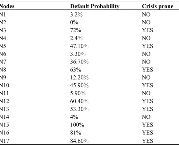
Table 6- Nodes’ Classification

Nodes Default Probability Crisis prone

N1 3.2% NO

N2 0% NO

N3 72% YES

N4 2.4% NO

N5 47.10% YES

N6 3.30% NO

N7 36.70% NO

N8 63% YES

N9 12.20% NO

N10 45.90% YES

N11 5.90% NO

N12 60.40% YES

N13 53.30% YES

N14 4% NO

N15 100% YES

N16 81% YES

16 The nodes 15, 16 and 17 seem to be the “perfect” combination for debt crisis occurrence. A high public debt, combined with a substantial external debt and an expansionary monetary policy (Node 15) leads inevitably to a default. Node 17 is associated with high inflation (more than 20%) and an external debt/ exports ratio exceeding 2.49. This level of external debt is also observed for node 16, combined moreover with a high service debt (exceeding 1.18 time the foreign reserves).

Admittedly, the external debt level is huge for the three nodes (observations classified on the right). But the default seems to be imminent when debt problems are associated with fiscal or/ and financial problems (node 15) or bad fundamentals like a high inflation rate (node 17). Even if an inflation rate exceeding 2% is not necessarily alarming, its interaction with a very high debt level leads to default.

On the other hand, even a moderate debt level can lead to default. Node 3 is classified on the left of the tree (with a low debt ratio). However, it is associated with a very high default probability (72%). Here, the vulnerabilities come from liquidity problems, i.e a short term debt exceeding the foreign reserves associated with high short term interest payments.

Node 5 is also classified on the left of the tree. However, it is associated with a quite high crisis probability (47%). In this case, crises are mainly due to liquidity problems (high debt and short term interest payments) combined with a monetary expansion and a very high external debt (exceeding 62% of the GDP). Similarly, crises classified in Node 8 mainly come from high inflation, low economic growth and high US interest rates.

Hence, we can classify observations into “crisis- prone” and “not- crisis prone” ones. To do so, we assessed the default probability for the whole sample (39.7%). Then, observations of a particular node are classified as “crisis prone” (if its default probability exceeds the sample’s one); or “not crisis prone” otherwise.

4-2-1 Classification of nodes :

17

 First Group of Nodes : Relatively sound fundamentals:

It consists in nodes classified as “not crisis prone”, i.e nodes 1, 2, 4, 6, 7, 9 11 and 14. Except for the Node 14, all observations classified in this group are associated with a moderate external debt, in terms of exports and GDP (respectively less than 2.49 and 0.85). Nodes 1, 2 and 4 are associated with a very low inflation rate (less than 10%), combined with a reasonable short term debt (less than 1.46 of foreign reserves) for the Node 1, with low short term interest payments for Node 2, and even an external debt ratio lower than 62% of GDP (Node 4). Otherwise, and even Node 7 suffers from inflation problems, interaction with low interest rates (less than 6%) and limited private credit growth (less than 25%) has offset the negative effect of high inflation and weak growth (lower than 2%). Similarly, Node 9 takes advantage from a quite high growth rate and an external debt lower than 54% of the GDP.

Node 14 seems to be an exception, in that it consists in the only group whose external debt is huge (more than 2.49 times the exports). However, the node 14 is not classified as « crisis prone ». In fact, only 4% of observations belonging to this node represent crisis episodes. This situation shows that a moderate inflation, associated with low debt service and weak long term public debt (in terms of GDP) appears to be sufficient to prevent crises, even if external debt is huge.

 Second Group of Nodes : Liquidity problems

It consists in observations classified within Nodes 3 and 5. In spite of moderate debt ratios, in terms of exports (less than 2.49) and GDP (less than 85%), the high level of short term debt in terms of GDP (more than 1.46) as well as short term interest payments exceeding the computed threshold have considerably increased crisis probability to 72% for Node 3.

 Third Group of Nodes : Solvency Problems :

18 However, Nodes 10 and 12, on the left of our classification tree, are also associated with solvency problems: an external debt ranging from 54% to 85% combined with an inflation rate exceeding 10% (Node 10); and an external debt in excess of 85% of GDP (Node 12).

For both nodes, the external debt ratio in relation to exports remains under the threshold (2.49). However, the use of this ratio is questionable because of problems related to exports valuation. Hence, Debt/ Exports ratio can be under- estimated simply because of hikes in global prices, which can be temporary, and this despite of the presence of high external debt levels.

 Fourth Group of Nodes : Pure Macro- economic problems :

Node 8 does not exhibit any evident vulnerability due to liquidity or solvency problems. However, node 8 is associated with a high default probability (68%) and classified hence as “crisis prone”. Here, external debt is inferior to computed thresholds, but interaction with high inflation rate (more than 10%), a weak economic growth (less than 2%) and high American interest rates (exceeding 6%) leads to crises.

4-2-2 Usefulness of this classification :

This application has three advantages. First, the computed thresholds can be used by international financial institutions, like IMF, to supervise countries. Any exceedance from thresholds should lead the IMF to warn the country’s government.

Second, this framework can play an important role in crisis prevention, in that if countries find themselves in a “not crisis prone” node, i.e nodes 1, 2, 4, 6, 7, 9, 11 and 14, default risk should be low. To be in these nodes, countries have to respect these nodes’ characteristics2. These governments should hence carry out fiscal, external debt, monetary and financial policies that keep them within this safe zone.

However, belonging to these nodes does not necessarily mean the absence of default risk. Admittedly, crisis probabilities are here low but they exist: this is the third purpose of this paper. In fact, any country out of the “red zone”, i.e our third group of nodes announcing solvency problems, is eligible to a financial support by the ILOLR, the IMF. According to the literature relative to LOLR, the latter should intervene only in case of liquidity crisis, never

19 solvency ones. Actually, the bailout of insolvent institutions never resolves their difficulties and leads to a waste of the lender’s resources. On the contrary, these institutions should be liquidated or restructured deeply. The same principle should be applied to countries: an insolvent country that finds itself in the third group of nodes cannot be bailout. In fact, financing is insufficient in case of insolvency; a deep structural adjustment should precede the financial support: this is the case of countries ineligible, or ex ante conditionality, suggested by the IMF to prevent and to manage crises. Indeed, any intervention of the IMF, in the form of international loans of last resort, will fail given that the ILOLR has not to manage a solvency crisis (Bagehot rules3).

On the other hand, even if a country respects eligibility rules and finds consequently itself in the first, second or fourth group of nodes, he can face a crisis. But here, crises are not solvency ones, they may result from international contagion, liquidity or macroeconomic problems needing adjustment; one can note the absence of external debt problems here. Hence, a country belonging to one of these groups would be eligible to a bailout in external liquidity from the IMF. The fact that the country does not belong to red zone shows that he respects IMF ex ante conditionality.

One should notice that the respect of eligibility criteria is not sufficient to prevent crises. However, it reduces default risk. In addition, a country which respects ex ante conditionality would be eligible to an ILOLR because of its solvency.

To sum up, this framework would be suitable not only for countries, seeing that it reduces default risk, but also for international financial institutions which may play the ILOLR role (here the IMF). The setting of rules with well defined thresholds would not only help the IMF to capture optimal intervention zones but also to act promptly. Celerity of intervention would in fact reduce probability of contagion beyond country’s frontiers.

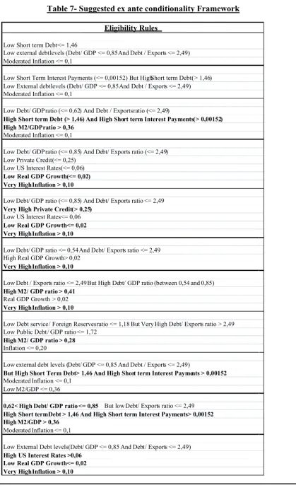
The ex ante quantified conditionality framework that we propose is shown in the Table 7.

3 _{The notion of LOLR dates from two centuries (Thornton, 1802; Bagehot, 1873). According to Bagehot, the}

20

Table 7- Suggested ex ante conditionality Framework

Eligibility Rules

Low Short term Debt _{<= 1,46}

Low external debt levels (Debt/ GDP <= 0,85 And Debt / Exports <= 2,49) Moderated Inflation <= 0,1

Low Short Term Interest Payments (<= 0,00152) But High Short term Debt(> 1,46) Low External debt levels (Debt/ GDP <= 0,85 A_{nd Debt / Exports <= 2,49)} Moderated Inflation <= 0,1

Low Debt/ GDP ratio (<= 0,62) And Debt / Exports ratio (<= 2,49)

High Short term Debt (> 1,46) And High Short term Interest Payments (> 0,00152) High M2/GDP ratio _{> 0,36}

Moderated Inflation <= 0,1

Low Debt/ GDP ratio (<= 0,85) And Debt/ Exportsratio (<= 2,49) Low Private Credit (<= 0,25)

Low US Interest Rates (<= 0,06)

Low Real GDP Growth (<= 0,02) Very High Inflation > 0,10

Low Debt/ GDP _{ratio (<= 0,85) And} Debt/ Exports ratio <= 2,49

Very High Private Credit (> 0,25)

Low US Interest Rates <= 0,06

Low Real GDP Growth <= 0,02 Very High Inflation _{> 0,10}

Low Debt/ GDP _{ratio <= 0,54 And Debt/ Exports ratio <= 2,49} High Real GDP Growth > 0,02

Very High Inflation _{> 0,10}

Low De_{bt / Exports ratio <= 2,49 But High Debt/ GDP ratio (between 0,54 and 0,85)}

High M2/ GDP ratio > 0,41

Real GDP Growth > 0,02

Very High Inflation > 0,10

Low Debt service / Foreign Reserves ratio <= 1,18 But Very High Debt/ Exports ratio > 2,49 Low Public Debt / GDP ratio <= 1,72

High M2/ GDP ratio > 0,28

Inflation <= 0,20

Low external debt levels (Debt/ GDP<= 0,85 And De_{bt / Exports <= 2,49)}

But High Short Term Debt > 1,46 And High Short term Interest Payments > 0,00152

Moderated Inflation <= 0,1 Low M2/GDP <= 0,36

0,62< High Debt/ GDP ratio <= 0,85 But low Debt/ Exports ratio <= 2,49

High Short term Debt _{> 1,46 And High Shor}t term Interest Payments > 0,00152 High M2/GDP > 0,36

Moderated Inflation <= 0,1

Low External Debt levels (Debt/ GDP _{<= 0,85 And De}bt/ Exports <= 2,49)

21

4-

Conclusions :

The ex ante conditionality framework developed in this paper is certainly quantitative, with well defined thresholds, but IMF intervention cannot be limited to these rigid numbers. It consists in a framework playing the role of a reference, not strict rules, like Maastricht Treaty.

Admittedly, holding an eligibility framework will help the IMF to act promptly. However, interventions should not be automatic, obeying to pre- determined thresholds. Judgment turns out also to be a decisive factor. In addition, and except factors assessed in our classification, i.e fiscal and external sustainability as well as financial soundness, other elements may play a very important role, like political variables, used for example by Manasse, Roubini and Schimmelpfennig (2003). It can include political rights, civil freedom rights, political constraints, years of parliamentary and presidential elections or electoral system. In sum, these variables may represent a proxy of country’s political uncertainty. Unfortunately, we were unable to collect this type of data, gathered by organizations like Freedom House which studies democracy’s extent in the world.

22

References

- AIZENMAN J. & LEE J. (2005), “International Reserves: Precautionary Vs. Mercantilist Views, Theory, and Evidence,” IMF Working Paper 05/198.

- AIZENMAN J. & MARION N. (2002), "International Reserve Holdings with Sovereign Risk and Costly Tax Collection", NBER Working Paper, nº w9154

- BAGEHOT W. (1873), Lombard Street : A Description of the Money Market, London, Kegan, Paul & Co. Eds.

- BECK R. & RAHBARI E. (2008), “Optimal reserve composition in the presence of sudden stops: the euro and the dollar as safe haven currencies”, ECB Working Paper 916.

- BUSSIÈRE M. & MULDER C. (1999), “External Vulnerability in Emerging Market Economies: How High Liquidity can Offset Weak Fundamentals and the Effects of Contagion,” IMF Working Paper 99/88

- CABALLERO R. & PANAGEAS S. (2004), “Contingent Reserves Management: An Applied Framework,” Working Paper, Federal Reserve Bank of Boston, N°05-2, septembre.

- CALVO, G. A. (1996), “Varieties of Capital-Market Crises”, forthcoming in The Debt Burden and its Consequences for Monetary Policy, G. Calvo and M. King (eds), London: MacMillan Press

- DE BEAUFORT WIJNHOLDS J. & KAPTEYN A. (2001), “Reserve Adequacy in Emerging Market Economies”, IMF Working Paper 01/43.

- DE BEAUFORT WIJNHOLDS J. (1977), « The Need for International Reserves and Credit”, Martinus Nijhoff, Leiden.

- DETRAGIACHE E. & SPILIMBERGO A. (2001), “Crises and Liquidity: Evidence and Interpretation”, IMF Working Paper 01/2, janvier

- EICHENGREEN B. & FRANKEL J. (1996), “The SDR, Reserve Currencies and the future of the International Monetary System”, dans “The Future of the SDR, in Light of Changes in the International Financial System”, Fonds Monétaire International, 18- 19 mars

- FLOOD R. P. & GARBER P.M. (1984), “Collapsing Exchange Rate Regimes: Some Linear Examples”, Journal of International Economics, Vol. 29, No. 1, 1- 13.

- FRANKEL J. & ROSE A. (1996), “Currency crashes in Emerging market: empirical indicators”, NBER N°5437, janvier

- FRENKEL J. (1978), “International Reserves: Pegged Exchange Rates and Managed Float”, in K. Brunner and A. H. Meltzer (eds.), “Public Policies in open Economies”, Carnegie- Rochester Series on Public Policy, Vol 9, 111- 40.

- FRENKEL J. (1983), “International Liquidity and Monetary Control”, in International Money and Credit: the Policy Roles”, Ed. George von Furstengerg, 65- 128, IMF - GABBI G., BOCCONI S., MATTHIAS M. & DE LERMA M. (2006), “CART

23 - GARCIA P. & SOTO C. (2004a), “Large Hoarding of International Reserves: Are they

worth it?” manuscript, Bank of Chile

- GEITHNER T. (2002), Assessing Sustainability, IMF, the Policy Development and Review Department, in consultation with the Fiscal Affairs, International Capital Markets, Monetary and Exchange Affairs, and Research Departments

- GREENSPAN A. (1999), “Currency Reserves and Debt”, Address at World Bank Conference on Trends in Reserve Management, Washington, avril.

- GRIMES A. (1993), "International Reserves under Floating Exchange Rates: Two Paradoxes Explained", The Economic Record, vol. 69, nº 207, 411-415

- GUIDOTTI P., STURZENEGGER F. & VILLAR A. (2004), On the Consequences of Sudden Stops, Economía, Vol. 4, N° 2, 171–203

- HELLER R. & KHAN M. (1978), “The Demand for International Reserves Under Fixed and Floating Exchange Rates”, IMF Staff Papers, Vol 25, décembre, 623- 49.

- HELLER R. (1966), “Optimal International Reserves,” Economic Journal 76, 296—311 - HUNG C. & CHEN J. (2009), “A selective ensemble based on expected probabilities for bankruptcy prediction”, Expert Systems with Applications, Volume 36, N° 3, Part 1, avril, 5297-5303.

- INTERNATIONAL MONETRAY FUND (1953), “The Adequacy of Monetary Reserves”, International Monetary Staff Papers, Vol III, N°2, octobre.

- INTERNATIONAL MONETRAY FUND (2000), « Debt and Reserve Related Indicators of External Vulnerability », SM/00/65 (23/03/2000)

- INTERNATIONAL MONETRAY FUND (2001), “Issues in Reserves Adequacy and Management”, IMF Board Paper. octobre

- INTERNATIONAL MONETRAY FUND (2009), IMF Report N° 09/329 , December - ISCANOGLU A., WEBER G. & TAYLAN P. (2007), “Predicting Default Probabilities

with Generalized Additive Models for Emerging Markets”, Graduate Summer School on New Advances in Statistics, METU, août 11-24.

- JEANNE O. & RANCIÈRE R. (2006), “The Optimal Level of International Reserves for Emerging Market Countries: Formulas and Applications » IMF Working Paper 06/229, octobre.

- JEANNE O. & RANCIÈRE R. (2006), The Optimal Level of International Reserves for Emerging Market Countries: Formulas and Applications, IMF Working Paper 06/229

- JEANNE O. (2007), “International Reserves in Emerging Market Countries: Too Much of a Good Thing?”, Brookings Papers on Economic Activity, Volume 38, janvier, 1-80. - KAMINSKY G. (2006), “Currency crises: Are they all the same?”, Journal of

International Money and Finance 25, 503-527.

24 - KIM J., LI J., RAJAN R., SULA O. & WILLETT T. (2005) “Reserve Adequacy in Asia Revisited: New Benchmarks Based on the Size and Composition of Capital Flows”, Claremont-Kiep Conference, novembre

- KOČENDA E. & VOJTEK M. (2009), “Default Predictors and Credit Scoring Models for Retail Banking”, CESIFO Working Paper N° 2862, décembre.

- KRUGMAN P. (1979), “A Model of Balance Of Payments Crises”, Journal of Money, Credit and Banking, Volume 11, N° 3, août, 311- 325

- LI J. & RAJAN R. (2005), “Can High Reserves Offset Weak Fundamentals? A Simple Model of Precautionary Demand for Reserves”, Lee Kuan Yew School of Public Policy Working Paper 13-05.

- LIZONDO J. & MATHIESON D. (1987), “The Stability of the Demand for International Reserves”, Journal of International Money and Finance, Vol 6, septembre, 251- 282

- MANASSE P., ROUBINI N. & SCHIMMELPFENNIG A. (2003), Predicting Sovereign Debt Crises, IMF Working Paper 03/221.

- MULDER C. (2000), “The Adequacy of International Reserve Levels: A New Approach”, In Risk Management for Central Bankers, edited by Steven F. Frowen, Robert Pringle, and Benedict Weller. London: Central Bank Publications

- OFFICER L. (1976), “The Demand for International Liquidity”, Journal of Money, Credit and Banking, août

- OLIVIERA J. (1971), “The Square- Root Law of Precautionary Reserves”, Journal of Political Econompy, vol 79, septembre- octobre, 1095- 1104.

- POLAK J. (1970), “Money: National and International”, International Reserves: Needs and Availability, Papers and Proceedings of a seminar at the IMF, June, IMF

- REDRADO M., CARRERA J., BASTOURRE . & IBARLUCIA J. (2006), “The economic policy of foreign reserve accumulation: new international evidence”, Working Paper 2006/ 14, ie | BCRA Investigaciones Económicas, Banque centrale de la République d’Argentine

- RODRIK D. & VELASCO A. (1999) “Short Term Capital Flows”, NBER Working Paper No. 7364, septembre.

- SACHS J., TORNELL A. & VELASCO A. (1996), “Financial Crises in Emerging Markets: The Lessons From 1995”, NBER WP 5576, mai

- SHCHERBAKOV S. (2002), "Foreign reserve adequacy: case of Russia", Fifteenth Meeting of the IMF Committee on Balance of Payments Statistics Canberra, Australia, October 21–25

- SKALA M., THIMANN C. & WÖLFINGER R. (2007), “The Search For Columbus’ EGG: Finding A New Formula To Determine Quotas At The IMF”, European central bank OCCASIONAL PAPER SERIES NO 70, août.

- SOTO C., Naudon A., López E. & Aguirre A. (2004), “Acerca del Nivel Adecuado de las Reservas Internacionales”, Banco Central de Chile Working Paper No. 267.

25 - Triffin R. (1960), “Gold and the Dollar Crisis”, yale University Press, New Haven - WILLET T. Nitithanprapas E., & Rongala S. (2004), “The Asian Crises Re-examined”,

Asian Economic Papers, Vol. 3, septembre, 32-87.

- WILLIAMS M., DE SILVA H., KOEHN M. & ORNSTEIN S. (1990), “Why did so many savings and loans go bankrupt?”, Economics Letters Volume 36, N° 1, mai, 61-66.

26

Appendix 1 Episodes of

Sudden stop

Country

S

udden stop Episodes

Argentina Bolivia Botswana Brazil Bulgaria Chile China Colombia Costa Rica Czech Republic Dominican Republic Equator Egypt El Salvador Guatemala Honduras Hungary India Indonesia Jamaica Jordan South Korea Malaysia Mexico Morocco Pakistan Panama Paraguay Peru Philippines Poland Romania South Africa Sri Lanka Syria Thailand Tunisia Turkey Uruguay Venezuela Vietnam

1980- 1982- 1989- 1994- 2001- 2002- 2008- 2010- 2011 1980- 1982- 1983- 1985- 1999- 2000- 2003- 2005- 2006 1977- 1979- 1981- 1986- 1987- 1993- 1998- 2001- 2003 1982- 1989- 1994- 2002- 2010- 2011

1991- 1994- 1996- 2003- 2009- 2012 1982- 1983- 1985- 1991- 1995- 1998- 2009

1983- 1986- 1987- 1991- 1998- 1999

1979- 1981- 1982- 1984- 1987- 1993- 1994- 1996- 2000- 2003- 2011- 2012 1996- 1997- 2003

1976- 1978- 1981- 1982- 1983- 1985- 1987- 1990- 1993- 1995- 1996- 2002- 2003- 2006-2011

1979- 1981- 1983- 1986- 1988- 1989- 1992- 1993- 1995- 1997- 1999- 2000- 2003- 2004- 2005- 2006- 2011

1983- 1987- 1990- 1999- 2002- 2003- 2006

1977- 1979- 1982- 1983- 1984- 1985- 1987- 1990- 1991- 1996- 1999- 2000- 2001- 2004 1979- 1980- 1982- 1984- 1986- 1988- 1990- 1992- 1994- 1995- 1999- 2002- 2004- 2005 1976- 1978- 1981- 1982- 1983- 1985- 1986- 1988- 1989- 1991- 1995- 1996- 1998- 2000- 2002- 2005- 2006- 2012

2010- 2011

1984- 1997- 1998- 2011

1977- 1978- 1983- 1985- 1986- 1988- 1992- 1995- 1997- 1999- 2002- 2003- 2006 1979- 1984- 1989- 1992- 1993- 1998- 2001- 2003- 2007

1986- 1997

1976- 1977- 1979- 1984- 1985- 1987- 1994- 1997- 1998- 1999- 2005- 2011 1982- 1983- 1987- 1994- 1995- 1998- 1999- 2004- 2006- 2011

1978- 1979- 1995- 2010 1998- 2009

1980- 1983- 1987- 1988- 1991- 2000- 2002- 2006 1981- 1982- 1985- 1987- 1988- 1999- 2004- 2006 1978- 1983- 1984- 1986- 1988- 1998- 2005- 2009 1979- 1981- 1983- 1985- 1997- 1998- 2001- 2004-2011 1994- 2009- 2011

1988- 1993 1985- 2009- 2010

1983- 1984- 1988- 1990- 1992- 1995- 1996- 2001 1989

1982- 1985- 1986- 1992- 1997- 2006- 2007- 2011 1979- 1983- 1985- 2007

1988- 1991- 1994- 1998- 2001- 2006

1981- 1983- 1984- 1985- 1988- 1987- 1990- 1991- 1995- 1996- 1998- 1999- 2001- 2002- 2004- 2009

27

Appendix 2 Definitions and Sources of Variables

I For the Sudden Stops episodes :

-Financial Account KA - Rela GDP

- Exchange rate - GDP Deflator

lie bjd (IFS) WDI (World Bank) line ae (IFS) line 99 bip4 _(IFS)

II For the parameters :

-Short term debt - Output Loss

- Retrun on reserves r - Ten-Year American Treasury Bonds

GDF (World Bank) WDI (World Bank)

line 60C IFS (3- month T- Bill rate)

(IFS line 61) - federal fund rate(IFS line 60B)

III- For the assessment of the sudden stop Probability π :

Debt variables -Short Term Debt (GDF) / GDP (WDI) -Public Debt (GDF) / GDP (WDI)

Exchange Rates -Real exchange rate deviation vis-à-vis HP trend (Hodrick- Prescott) IFS line rf

-Dummy variable for the exchange regime : 1 for fixed regime and 0 for floating one (Reinhart et Rogoff, 2004, updated) ;

International Trade -Trade openness : Exports (IFS line 70) + Imports (IFS line 71)/ GDP (WDI)

-Terms of Trade growth (IFS line 74/ IFS line 75)

American Interest Rates -US Treasury Bonds interest (IFS line 60C)

-Interest rates change of US Treasury Bonds (IFS line 60C)

Financial Development : -Bank Deposits (IFS line 24 + 25)

- Banks- CB : IFS (lines 22A+22B+22C+22D)/ (12A+12B+12C+12D)

-M2 Multiplier: M2 (IFS line 34 + 35)/ M0 (IFS line 14)

-M2 / GDP (WDI) -M3 IFS line 59MC

-Market Capitalization / GDP (Emergent Market DataBase)

-Credit for Private Sector IFS line 22D / GDP (WDI)

Business cycle -Real GDp Growth (WDI)

28

-Domestic Real Credit growth IFS line 32/ CPI IFS line 64

Financial Account Openess -Gross Capital inflows/ GDP: lines IFS 78bed, 78bgd, 78bmd, 78bnd, 78bxd, 78bid ;

-Total of gross capital inflows and outflows IFS 78bdd, 78bfd, 78bkd, 78bld, 78bwd, 78bhd

Stocks of foreign assets and liabilities -Foreign Direct Investments (IFS line 78bed+ 78bdd) / Liabilities Stocks

-Foreign Liabilities (IFS line 16c + 26c + 4d)/ GDP (WDI)

-Net Foreign Assets (IFS line 31n) / GDP (WDI) Other variables -Foreign Liabilities (IFS line 26c) / M2 (IFS line 34 +

29

Appendix 3- Variables used in CART

Variables Source

I-External Sustainability:

Total External Debt / Exports (DEBT_X) GDF

Total External Debt / GDP (DEBT_GDP) GDF

Debt Service/ GDP (DEBTSERVICE_GDP)

Debt Service / Foreign Reserves (DEBTSERVICE_RC)

GDF

GDF and WDI Short Term Interest Payments / GDP (IPST_GDP) GDF and WDI Short Term Debt/ Foreign Reserves (DCT_RC) GDF and WDI

Exports (EXPORTS) GDF

Current Account / GDP (CURRENT) GDF and WDI

II- Fiscal Sustainability

:

Fiscal Deficit / GDP (FISCALCASH) GFS

PPG/ PIB (PPG_GDP) GDF

Public/ PIB (PUBLIC_GDP)

III- Financial Sector Soundness :

Credit to private sector (PRIVATECREDIT) IFS line 22D / GDP (WDI)

M2/ GDP (M2_GDP) WDI

M2 Multiplier (MULTIM2) IFS lines (34+35) /IFS line 14 Bank Deposits (DEPOSITS) IFS lines (24+25) /IFS line 64 Domestic Credit / GDP (DOMESTIC) (IFS line 52 / IFS line 64) / IFS

line 99 IV- Macroeconomic Variables :

Domestic Currency Overvaluation (TCR) Real Exchange Rate deviation from HP (Hodrick- Prescott) filter International interest rates (USI) IFS line 60 / IFS line 64

Real GDP growth (REALGDP) WDI

30

Appendix 4: Presentation of the CART methodology

The data mining concept is nowadays a popular tool of information management. It’s commonly used in many fields where decision taking is very important, mainly finance (credit scoring), loans management and financial forecasts.

A clasSification and regression tree is a structure with the form of a tree, splitting a set of input observations, on the basis of certain features, into narrower sets. A decision tree stocks certain classification rules into branches nodes, in order to gather similar observations of the sample in the same node (or leaf).

CART has the advantage of intercepting all interaction effects existing between the different variables, mainly when such interactions represent very important determinants of crises occurrence. CART takes into account the non-linearities and the complementarity of explaining variables.

31

Appendix 5: Noise to Signal Ratio (Kaminsky & Reinhart, 1999)

The noise- to-signal ratio can be defined using the matrix below:

-If the indicator signals a crisis and there’s effectively a crisis within the 24 months following this signal (Cell A), the signal is considered exact ;

-If the indicator signals a crisis but no crisis happens within the 24 months following this signal (Cell B), the signal is considered a false alert and called noise.

Hence, a perfect signal belongs to cells A or D.

The noise-to-signal ratio for any indicator is given by the number of entrees :

An indicator with a high number of noises would have few entrees in A and D celles, but many ones in B and C.

Crisis happening within the 24 months

No crises happening within

the 24 months

The indicator transmits a signal A B

The indicator doesn’t transmit a signal