Dispersive detection of radio frequency dressed states

arXiv:submit/2240916 [physics.atom-ph] 25 Apr 2018

Sindhu Jammi, Tadas Pyragius, Mark G. Bason, Hans Marin Florez, and Thomas Fernholz∗

School of Physics & Astronomy, University of Nottingham, University Park, Nottingham NG7 2RD, UK (Dated: April 25, 2018)

We introduce a method to dispersively detect alkali atoms in radio-frequency dressed states. In particular, we use dressed detection to measure populations and population differences of atoms prepared in their clock states. Linear birefringence of the atomic medium enables atom number detection via polarization homodyning, a form of common path interferometry. In order to achieve low technical noise levels, we perform optical sideband detection after adiabatic transformation of bare states into dressed states. The balanced homodyne signal then oscillates independently of field fluctuations at twice the dressing frequency, thus allowing for robust, phase-locked detection that circumvents low-frequency noise. Using probe pulses of two optical frequencies, we can detect both clock states simultaneously and obtain population difference as well as the total atom number. The scheme also allows for difference measurements by direct subtraction of the homodyne signals at the balanced detector, which should technically enable quantum noise limited measurements with prospects for the preparation of spin squeezed states. The method extends to other Zeeman sublevels and can be employed in a range of atomic clock schemes, atom interferometers, and other experiments using dressed atoms.

I. INTRODUCTION

Radio-frequency (RF) dressing of atoms in magnetic traps provides robust and very versatile control of the ex-ternal degrees of freedom. This technique is used in a va-riety of cold-atom experiments, see [1] for a recent review. The dependence of the trapping potential on magnetic field amplitudes in the RF regime renders dressed traps robust against some low-frequency, environmental field noise. The first atom-chip based beam splitter for matter waves was demonstrated with this method [2]. Versatility comes from the dependence of the trapping potential on the polarization of the RF field relative to the local static field; this provides greater design freedom compared to quasi-static magnetic traps. Experiments and propos-als for interesting trap geometries include lattices [3, 4], rings [5–8], and hollow traps shaped as spheres [9], cylin-ders [10], and tori [5]. Species- and state-dependent con-trol becomes possible in some scenarios [8, 11], because the trap defining RF polarization component depends on the atomicg-factor. Such control provides prospects for quantum simulations of many-body physics as well atom interferometers without any free propagation [12].

In this paper, we present a method for dispersive de-tection of atoms that benefits directly from the intrin-sic modulation of the atomic signal via phase-locked spin precession. Dispersive light-matter interaction at a very low technical noise level resulting from operation at radio-frequencies is a prerequisite for quantum-non-demolition (QND) measurements in a range of vapour cell experiments with very large atom numbers (n≈1012₎

and consequently low relative quantum noise, including spin-squeezing [13], deterministic quantum memory [14], and teleportation [15]. Such QND measurements also

∗_{corresponding author: thomas.fernholz@nottingham.ac.uk}

play a role in atom interferometry where it is desirable to lower the quantum projection noise [16] inherent to any atomic magnetometer [17], clock [18], or interferom-eter [19] by using spin-squeezed states [20, 21] or other non-classical states [22] as inputs. Destructive detection methods, e.g., based on fluorescence imaging, are rou-tinely used to achieve atomic shot noise limited detection for small [23] to large ensembles [24]. They are, however, not capable of generating spin squeezing needed to lower the projection noise. In contrast, dispersive measure-ments based upon off-resonant atom-light interactions enabled experimental demonstration of 18-20 dB spin-squeezing [25, 26]. These experiments used high-finesse optical cavities to achieve strong atom-light interaction with low atom numbers, and require significant technical effort to stabilize to sufficient robustness. In particu-lar, measurements on standard atomic clock states, i.e. magnetic field insensitive states with magnetic quantum numberm=0, do not seem compatible with the relatively simple low-noise techniques used with vapour cells that are based on the Faraday effect and polarimetric common path interferometry with RF sideband detection. Here, we demonstrate that another type of birefringence, the Voigt effect [27], can in principle be used to detect these states by similar means. We perform two-state detec-tion to observe Rabi cycles with low technical noise and discuss prospects for achieving quantum limited perfor-mance.

The paper is organized as follows. In section II, we describe dispersive interaction in the context of radio-frequency dressing. this treatment predicts detected sig-nals at harmonics of the dressing frequency. Section III reports experimental results using our method and dis-cusses the observed noise behaviour as well as future ex-tensions. SectionIVpresents our conclusions. Details on dispersive interaction and quantum mechanical interac-tion strengths are given in appendices A and B.

II. RADIO-FREQUENCY DRESSED, DISPERSIVE LIGHT-MATTER INTERACTION

A. Circular and linear birefringence

In this section, we review the dispersive atom-light in-teraction arising from off-resonant laser light propagating through an atomic medium. In particular, we consider linear birefringence of an ensemble that has been pre-pared in a certain Zeeman sublevel, e.g., in an atomic clock state.

The basic principle can be understood by considering the simplifed example in Fig. 1 for an atom with total spinF =1 and an optical transition to an excited state withF′=1. Off-resonant light fields experience little ab-sorption but acquire a phase-shift proportional to transi-tion strength and atom number. If atoms are prepared in a single Zeeman sublevel, the interactions withπ- andσ -polarized fields will differ, described by different Clebsch-Gordan coefficients. For the depicted case of the quanti-zation axis chosen alongey and atoms prepared in state ∣F =1, Fy=0⟩, the interaction withπ-polarized light, i.e., linearly polarized along the y-axis, completely vanishes because of selection rules considering only coupling to excited states withF′=1. Any orthogonal polarization, however, experiences a phase shift. Light propagating along ez, polarized at 45° with respect to the x, y-axes becomes elliptically polarized, and this provides a means to measure atom number.

E

∆

σ− π σ+ F′₌1

F ₌1

Fy −̵h 0 h̵

σ

-p

o

l

.

π_-pol.

ey

atom

s

ˆ Sy=c₂nˆ⤡

ˆ Sx,z≈0

ˆ Sz′

x

y

z

FIG. 1. Linear birefringence. An example level scheme for an F = 1 → F′ = 1 transition is shown on the left. Only

σ-transitions are allowed for atoms in_∣1,0_⟩, and correspond-ing polarization components of near-resonant light will ac-quire a phase shift proportional to atom number. An initial 45°-polarization as shown on the right will become elliptical, measured by Stokes operator ˆSz′ at the output.

For a more comprehensive description of the inter-action, the atomic multi-level character and arbitrary light polarization must be included. As detailed in Ap-pendixA, these can be captured by a frequency depen-dent polarizability tensorαthat describes the medium, and Stokes operators that describe the photon flux.

The dispersive interaction can be decomposed into spin dependent, irreducible tensor components of different rankk=0,1,2. The components are associated with cor-responding polarizability contributions α(_Fk), which de-pend on the total spin quantum numberF of the atomic ground state hyperfine level. The 87_{Rb atoms used in}

this work have nuclear spin I = 3/2, and consequently, ground state levels withF =1,2. For atoms driven near the D1 lines (J=J′=1/2) the contributions, see general expressions in Eqs.A5andA6, are explicitly given by

α(₁0)=αJ′ 6 [

1 ∆1,1+

5 ∆1,2]

, α(₂0)= αJ′ 2 [

1 ∆2,1 +

1 ∆2,2]

,

α(11)=

αJ′

8 [ − 1 ∆1,1+

5 ∆1,2]

, α(21)=

αJ′

8 [ − 3 ∆2,1 + −

1 ∆2,2]

,

α(_F2)=αJ′ 8 (−1)

F_[ 1 ∆F,1+ −

1 ∆F,2]

, (1)

with the far-detuned, scalar polarizability coefficient αJ′ = ǫ₀λ3

J′ΓJ′/8π2, which depends on the D1-line

pa-rameters ΓJ′ = 2π×5.75 MHz and λ_J′ = 795 nm. We

defined detunings ∆F,F′ = ω_L−ω_F,F′ of the light field

with respect to the optical F → F′ _transition frequen-cies. The ground- and excited state hyperfine splittings are ∆2,F′ −∆_1,F′ ≈ 2π×6835 MHz and ∆F,₂−∆F,₁ ≈

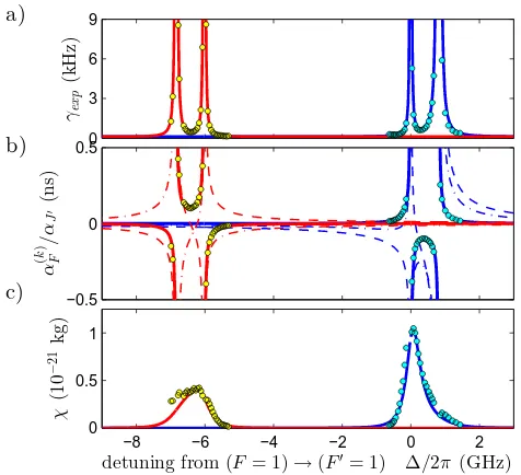
2π×817 MHz. This large difference relative to the small probe detuning used in our experiments, justifies treat-ing the twoF = 1,2 sub-ensembles independently. The frequency dependence of the polarizability contributions and expected spontaneous decay coefficients, together with experimental data, are shown in Fig.2.

The scalar polarizabilities (k = 0) do not affect the polarization of a light beam. The higher order terms are linked to spin-dependent circular(k=1) and linear

(k = 2) birefringence, named Faraday and Voigt effect, respectively. We assume a quasi one-dimensional sce-nario with cross sectionA, and describe a coherent laser beam, polarized at 45°, by photon fluxSy. Stokes opera-tors ˆSx,z≈0 quantify quantum mechanical uncertainty of the input beam’s polarization, see Eq.A2for definitions. For small optical phase shifts(≪1 rad), neglecting light retardation and back action onto the traversed atomic ensemble, the polarization rotation and ellipticity of the output beam are measured by the operators

ˆ

S_x′ =Sˆx−g(

1₎

F Sy∑ i

ˆ

Fz,i (2)

ˆ

S_z′=Sˆz+g(

2₎

F Sy∑ i (

ˆ

F_x,i2 −Fˆ_y,i2 ), (3)

0 3 6 9

γex

p

(k

Hz

)

a)

−0.5 0 0.5

α

(

k

)

F

/

α

J

′(n

s)

b)

−8 −6 −4 −2 0 2

0 0.5 1

detuning from (F = 1)→(F′_{= 1) ∆/2}

π (GHz)

χ

(10

−

21

kg

)

c)

FIG. 2. Frequency dependence of spontaneous emission and atomic polarizability. a) Experimental decay ratesγexp

(cir-cles) for both clock states using light polarized at 45°with re-spect to the quantization axis. The expected behaviour (solid lines) for atoms in F =1 (blue group, right) andF =2 (red group, left) is based on measured light powers and beam sizes with 30% correction to one of the probe lasers, possibly due to slight misalignment. b) The k-rank tensor contributions to the off-resonant D1 line polarizability (dashed, dash-dotted, solid lines fork₌0,1,2). A single fit parameter was used to scale the measured linear birefringence (circles) to match the expected behaviour of the k ₌2-terms. c) Theoretical, off-resonant approximation and experimental data for the figure of meritχ= (α(F2)/αJ′)2_⋅I₀/γ, i.e., the ratio of squared polar-izability to decay coefficient (per beam intensityI0=P/A),

which determines the maximally achievable, signal-to-noise-power-ratio for fixed on-resonant optical density, see Eq. B13.

For known spin states, both signals can in principle be used to measure atom numbers. If all nF atoms in theF-manifold are in the same state, we can express the expectation values by individual atomic operators as

⟨_Sˆ′ x⟩=−g(

1)

F SynF⟨Fˆz⟩, (4)

⟨_Sˆ′ z⟩=g(

2)

F SynF⟨Fˆx2−Fˆ

2

y⟩. (5)

For standard clock states, which have one zero spin component (m =0), the population cannot be detected by measuring Faraday rotation due to lack of any ori-entation, i.e., ⟨Fˆ⟩ = 0. But for atoms in an eigen-state of the ˆFy-operator, linear birefringence is pro-portional to ξF(Fy) = ⟨F, Fy∣Fˆx2−Fˆy2∣F, Fy⟩ /̵h2. The moment ξF(m) = (F(F +1) −3m2)/2 is extremal for m = ±F as well as for m = 0 (bosons) or m =

±1/2 (fermions). Intermediate Zeeman substates hibit smaller linear birefringence, which becomes ex-actly zero only in rare cases including ∣0,0⟩,∣1/2,±1/2⟩,

∣3,±2⟩,∣25/2,±15/2⟩,∣48,±28⟩,∣361/2,±209/2⟩etc.

B. Adiabatic radio-frequency dressing In this section, we outline the principle of adiabatic RF dressing and discuss its effect on the measurements of atomic observables.

The magnetic fields that we use in our experiments are generally weak enough to neglect second order Zeeman splitting within each hyperfine manifold. In this case, RF dressing can simply be described as a rotation of an effective magnetic fieldBeff that combines the effects of

real fields and fictitious forces in a rotating frame. For slow enough rotation of this effective field with respect to the rotating frame, the atomic spin will adiabatically follow and precess about the direction of the effective field with constant spin projection along that direction.

To first order, the time-dependent interaction Hamil-tonian of an atom with spinFof constant magnitude in a magnetic field with static and oscillatory components is given by

ˆ

H =µB_̵gF

h Fˆ⋅(BRF(ωt)+BDC), (6) whereµB is the Bohr magneton andgF is the Land´e fac-tor. The oscillating part can best be expressed in terms of spherical polarization components. Choosing BDC =

BDCez and using the spherical basise±=(ex±iey)/√2 andeπ=ez, we can write

BRF(ωt)=Re[(B₊e₊+B₋e₋+Bπeπ)e−iωt]. (7)

Using corresponding spin components with the conven-tional normalization of raising and lowering operators

ˆ

F_±=Fˆx±Fˆy, the Hamiltonian is expressed as

ˆ

H= µBgF 2̵h [(

B₊

√

2 ˆ F₊+B√−

2 ˆ

F₋+BπFˆz)e−iωt

+BDCFˆz]+h.c. (8)

We transform to a frame rotating about the z-axis at frequency ω with a given phase ϕ, such that ˆHrot =

ˆ

UHˆUˆ−1+_ih̵∂ ∂tUˆUˆ−

1_{, using the unitary transformation}

ˆ

U_±(t)=ei(±ωt+ϕ)Fzˆ /̵h, (9)

where the sign of frequency is chosen equal to the sign of the Land´e factor gF, which determines the sense of rotation that is required to dress atoms resonantly. Using the identity eαFzˆ Fˆ±e−α

ˆ

Fz _{= e}±α_Fˆ

±, the rotating frame Hamiltonian becomes

ˆ Hrot± =

µBgF 2̵h [

B_∓e∓iϕ

√

2 ˆ

F_∓e−2iωt+BπFˆze−iωt (10)

+B±_√e±iϕ 2

ˆ

F_±+(BDC−Bres)Fˆz]+h.c.,

If the RF field is polarized purely in the e_± direction that corresponds to the Larmor precession, i.e., B_∓ = Bπ = 0, atoms will exhibit the same behavior as in an apparently static, effective field

B±_eff =1 2(B±e

±iϕ_e

±+c.c.)+(BDC−Bres)ez, (11)

described by the corresponding effective, rotating frame Hamiltonian

ˆ Heff± =

µBgF

̵

h Fˆ⋅B ±

eff. (12)

In particular, an atomic spin will adiabatically follow the effective field’s orientation provided that any reori-entation with ˙Beff,⊥ =Ω×Beff occurs at a rate that is

much slower than the effective Larmor frequency, i.e., for

∣Ω∣≪µBgF∣Beff∣/̵h. When other RF-polarization

com-ponents are present, the rotating wave approximation can be used, thus neglecting the fast oscillating terms of ˆHrot as long as ω ≫ µBgF∣Beff∣/̵h [31]. The

result-ing behaviour remains the same apart from second order energy shifts [32].

We now consider the specific transformation of atomic spin operators when an eigenstate of ˆFz, initially pre-pared in a static field along thez-direction, is dressed by adiabatically changing the components of the effective field. For the purpose of this paper, we assume an RF field that is linearly polarized in thex, y-plane, described by

BRF(ωt)=BRFcosωt⋅(excosϕ+eysinϕ), (13)

for which caseB_±=BRFe∓iϕ/ √

2 andBπ=0. The phase ϕ describes the direction of field oscillation and deter-mined our above choice of phase for the rotating frame. Consequently, we find for either effective field

B±eff =

BRF

2 ex+(BDC−Bres)ez. (14)

The initial state∣F, Fz⟩is an eigenstate of ˆU±(t)and ap-pears identical in both laboratory and rotating frame. ForBRF=0 it is an eigenstate of either frame’s

Hamilto-nian and differs only in its evolution of dynamical phase or its quasi-energy, which we can ignore for our purposes. Upon changing the effective field, we obtain the adiabatic state by applying the corresponding rotation about the (rotating)y-axis according to

∣Ψrot⟩=eiθ ˆ

Fy_{∣F, F}

z⟩, (15)

by an angle

θ=π 2 −tan

−1BDC−Bres

BRF/2

. (16)

The same state in the laboratory frame is then given by

∣Ψ(t)⟩=Uˆ_±−1(t)∣Ψrot⟩. (17)

Finally, we can express any laboratory frame atomic ob-servable ˆO using

⟨Ψ(t)∣Oˆ∣Ψ(t)⟩=⟨F, Fz∣Rˆ±OˆRˆ−±1∣F, Fz⟩, (18) ˆ

R_±(t)=e−iθFyˆ Uˆ_±(t). (19)

The result is a time-dependent geometrical rotation of coordinates given by the explicit transformation

ˆ

F′(_t)_=Rˆ_±(_t)FˆRˆ−_±1(t)=R_±(t)Fˆ (20)

=⎛⎜

⎝

cosθcosφ_±(t) −sinφ_±(t) −sinθcosφ_±(t) cosθsinφ_±(t) cosφ_±(t) −sinθsinφ_±(t)

sinθ 0 cosθ

⎞ ⎟ ⎠F,ˆ

where we defined R_±(t)= R_z(φ_±(t))R_y(−θ)as a com-bination of rotations about coordinate axes according to Rkv = ek(ek⋅v)(1−cosα)+vcosα+ek×vsinα (Ro-drigues’ rotation formula) and the time dependent angle φ_±(t)=±ωt+ϕ.

C. Linear birefringence of dressed eigenstates To consider different experimental geometries, in par-ticular for light propagation parallel or orthogonal to the static field, we use rotated light coordinates, expressed by a general rotation matrixM, such that (x′, y′, z′)T = M(x, y, z)T. Using Eq. 3, linear birefringence of eigen-states of the dressed Hamiltonian is then measured by

ˆ

Sz′(t)=Sˆ_z′(t)+g(2)

F Sy nF

∑

i=1[

ˆ F′2

y′_,i(t)−Fˆ′ 2

x′_,i(t)]

=Sˆz′(t)+g(2)

F Sy nF

∑

i=1

ˆ

FT_i Q_±Fˆ_i, (21)

introducing the quadratic form

Q_±=RT_±(t)MT⎛⎜

⎝

−1 0 0 0 1 0 0 0 0

⎞ ⎟

⎠MR±(t). (22)

Since the matrixQ_±is symmetric and the expectation values of mixed anti-commutators vanish for the original state⟨F, Fz∣ {Fˆj,Fˆk} ∣F, Fz⟩j≠k =0, the expression for the expected signal from an ensemble of identically prepared atoms reduces to the trace

⟨_Sˆ_z′(t)⟩=g(2)

F SynF

3 ∑

j=1

⟨F, Fz∣Qj,j_± Fˆj2∣F, Fz⟩, (23)

which can be expressed in terms of spectral RF compo-nents as

⟨_Sˆ′_z(_t)⟩_=g(2) F SynF

ξF(Fz)̵h2 2

2 ∑

n=0

hn(θ)einωt+c.c. (24)

−3 −2 −1 0 1 2 3 −1

0 1

com

p

on

en

t

h

′ k

field ratio (BDC−Bres)/BRF

FIG. 3. Principal behaviour of zeroth (dashed red, n =0), first (dash-dotted green, n ₌1) and second (solid blue, n₌ 2) harmonic signal components across RF resonance for the orthogonal case (β₌ π_/2) plotted as h′n = (±i)n

√

2hn with ϕ=0,α=π/4.

already described by ϕ. We choose sequential rotations M=Rx(α)Ry(β)=Ry′(β)R_x(α)leading to the result

(h0, h1, h2)T(θ)= (25)

⎛ ⎜⎜ ⎜ ⎝

1₊3 cos 2θ

4 (

cos2β

2 −

(3−cos 2β)cos 2α

4 )

sin 2θ(cosα₂sin 2β∓i(3−cos 2₄β)sin 2α)e±iϕ −sin2θ((3−cos 2β)cos

2

α+2 cos 2β

4 ∓i

sinαsin 2β

2 )e± 2iϕ

⎞ ⎟⎟ ⎟ ⎠

.

For the parallel settingα=β=0, the chosen coordinate systems for atomic and light variables coincide. In this case, the spectral components reduce to

⎛ ⎜ ⎝

h0

h1

h2 ⎞ ⎟ ⎠_∥(θ)=

⎛ ⎜ ⎝

0 0

−e±2iϕ_sin2

θ

⎞ ⎟

⎠. (26)

A setting with light propagation orthogonal to the static field is described by β =π/2. In this case, α de-scribes a rotation of beam polarization, with α= 0 for unchanged polarization, i.e., at 45○ _{with respect to the} static field. The amplitudes of the spectral components are then given by

⎛ ⎜ ⎝

h0

h1

h2 ⎞ ⎟ ⎠_⊥(θ)=

⎛ ⎜ ⎝

−1

4(1+3 cos 2θ)cos 2α ∓ie±iϕsin 2θsin 2α −1

2e± 2iϕ_sin2

θcos 2α

⎞ ⎟

⎠. (27)

The principal behaviour of these functions across RF res-onance is shown in Fig.3.

The results show that due to the axial symmetries of both the setup and the initial state, a parallel measure-ment only produces signals at the second harmonic, i.e., at frequency 2ω. This setting also leads to the maxi-mum possible signal oscillation with full swing between ±Smax=±g(

2)

F SynFξF(m)̵h2when the RF resonance con-dition θ =0 is met. The orthogonal setting with α=0 contains a DC part that is reminiscent of undressed de-tection with off-resonant amplitude Smax and leads to

a weaker signal at 2ω on resonance with an amplitude swing between 0 and −Smax. In both cases, a signal at

frequency ω arises only due to misalignment or rotated light polarization, with a zero crossing at resonance.

For detection of atomic population, the variations in signal strength will become important. Both, changes in magnitude of the static field BDC, which shifts the

resonance condition, as well as field rotations or equiv-alent beam misalignment affect the resonant 2ω-signal only to second order. Since the RF amplitude has no effect, it is advantageous to use higher RF amplitudes to broaden the resonance. The signal becomes less sensi-tive to fluctuations of external magnetic fields reducing the requirements for magnetic field shielding. A limit to this strategy will be imposed by effects from second order Zeeman splitting, which we do not analyze here.

III. EXPERIMENTAL REALISATION A. State preparation

We apply our detection method to an ensemble of ap-proximately 108 87_{Rb atoms, which we prepare in}

su-perpositions of the two clock states ∣F=1, mF =0⟩ and

∣F=2, mF =0⟩by driving the clock transition with a res-onant microwave pulse of variable duration.

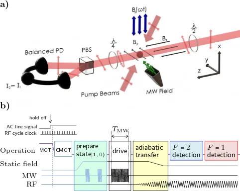
A sketch of the experimental setup is shown in Fig.4 a). In order to start from a pure state, we use an optical pumping and cleaning sequence to initially pre-pare atoms in∣F=1, mF =0⟩. After releasing a cloud of atoms from a standard, transiently compressed magneto-optical trap [33], we perform magneto-optical molasses cooling while we ramp up a weak magnetic field in they-direction

a)

b)

hold off AC line signal

RF cycle clock TMW

Operation MOT CMOT prepare

state∣1,0⟩ drive

adiabatic transfer

F=2

detection

F=1

detection Static field

MW RF

to≈0.3 G. We then replace the standardF=1→F′=2 repumping beam by a pair of counterpropagating, π -polarized beams tuned near theF=1→F′=1 transition on the D1 line for optical pumping. We use an intensity

of 80µWcm−1 _{and a red detuning of}−_{30 MHz to reduce}

re-absorption of scattered photons. This method contin-ues to provide cooling and avoids directional forces while atoms accumulate in the now dark∣1,0⟩state. After a pe-riod of 6 ms and sequential switch-off of first pump then cooling beams, we achieve(70±5)% population in∣1,0⟩ with a final temperature of(80±10)µK and the remain-ing atoms populatremain-ing the ∣1,±1⟩ states. Purification of the state is achieved by coherent transfer of atoms from

∣1,0⟩to ∣2,0⟩ using a resonant microwaveπ-pulse emit-ted from a sawed-off waveguide and a raised magnetic field of≈0.5 G, followed by a short pulse from the orig-inal repumping beam and a second microwave π-pulse, converting ∣2,0⟩ back to ∣1,0⟩. Incoherently transferred atoms then populate only F = 2 levels. We push these away from the cloud by shining a single resonant beam on the cyclingF =2→F′=3 transition on the D2-line,

leaving only the purified∣F =1, mF=0⟩state.

B. Dressed state detection

Figure4 b) shows the experimental sequence for state preparation, dressing and state detection. While the pu-rified ensemble is in free fall, we apply a resonant mi-crowave pulse for a variable durationTMWto drive

high-contrast Rabi cycles and prepare superpositions of the two clock states. Atoms are then adiabatically dressed with a magnetic RF field in the x-direction with fre-quencyω =2π×180 kHz, generated by an external res-onant coil. The RF field amplitude is ramped up to ≈ 15 mG over 4 ms while the static magnetic field is ramped down to a magnitude of BDC ≈260 mG, which

tunes the atomic Larmor frequency near resonance. For most experiments, the static field is simultaneously ro-tated from they-direction into thez-direction. This pro-cedure maintains the magnitude of the total collective spin as well as its alignment with the effective field such that the initial atomic spin projection Fy = 0 then ro-tates within thex, y-plane. While the total populations within each F-manifold remain unchanged, the atomic state then obeys Fxcos(ωt)±Fysin(ωt)= 0, where the sign of rotation depends on the state-dependent Land´e factorgF.

We use two-color detection to distinguish populations in the two hyperfine manifolds. The two D1-line

op-tical frequencies are detuned by −400 MHz from the F = 2 → F′= 2 transition and by +240 MHz from the F = 1 → F′ = 1 transition, respectively, avoiding two-photon resonance. Due to their separation of≈6.7 GHz, the interaction of each field with the atomic cloud is dominated by population in one of the two hyperfine states. The beams have perpendicular, linear polariza-tions and are combined with a Wollaston prism to

co-0 1 2 3 4 5 6 7

−1 0 1

ac

si

gn

al

U

(

t

)

(V)

timet(ms)

−0.5 0 0.5

|

˜

u1,

2

(

t

)

|

(m

s

−

1

/

2)

c) 0 5 10 15 20 25

−0.3 −0.2 −0.1 0

si

gn

al

U

(

t

)

(V)

b)

0 100 200 300 400

−60 −40 −20 0

frequencyf (kHz)

SU

U

×

1

kHz

(d

B

m

)

a)

FIG. 5. Typical experimental signals. a) Single-sided, power spectral density of the amplified, high-pass filtered signal. Atomic signals arise atωand 2ω. b) Direct signal forF₌2, recorded during a sweep of static field strength across the RF resonance in the orthogonal setting. Atoms are removed before a second probe pulse is used to determine the signal offset from imperfect detector balance (dashed line). The sig-nal matches the theoretical response but shows probe induced decay. c) Amplified signal for two-color measurement of both state populations in the parallel setting. Envelopes of the used temporal mode functions ˜u1,2(t)are shown in red (first

pulse,F=2) and blue (second pulse,F=1).

detec-tor signals together with a signal spectrum, which shows that signals arise at 180 kHz and 360 kHz above a noise floor that is limited by photon shot noise at frequencies above≈150 kHz. At lower frequencies, the spectrum is dominated by (ac-filtered) square-pulse transients from imperfectly balanced detector signals. As expected, the main contribution to the RF signal is found at frequency 2ω. We also detect signals at frequencyω in case of geo-metric misalignment.

The raw signals are processed via digital lock-in de-tection. As can be seen in Fig. 5 c), the atomic sig-nals decay due to spontaneous emission induced by the probe beams. We obtain signal values proportional to state populations by extracting spectral mode ampli-tudes m1,2 = ∫u∗1,2(t)U(t)dt from the RF signal U(t) with L2_{-normalized temporal mode functions u}

1,2(t) =

˜

u(t)e2i(ωt±ϕ). In the case of square laser pulses of dura-tionT, their envelopes take the form

˜ u(t)=⎧⎪⎪⎨⎪⎪

⎩

√ ₂

γ

1−e−2γTe−γt, if 0≤t≤T

0, otherwise, (28)

with experimentally determined, probe power dependent decay rates γ. For higher probe powers, we use shaped pulses to avoid light-shift induced excitation of Larmor precession about the effective field, which may occur at Rabi frequency ΩRF corresponding to the RF field

am-plitude. For shaped pulses, we use heuristically adapted mode-functions (see shaped pulses in Fig. 11). Our fre-quencies and mode functions allow for slowly varying en-velope approximations with negligible spectral overlap of signals from different harmonics.

The mode amplitudes are referenced to the input light according tom′1,2=m1,2/P1,2, whereP1,2 are the

simul-taneously measured, pulse-averaged probe powers, pro-portional to Sy. This is used to correct for small light power fluctuations, neglecting power-dependent changes in the decay rates. We extract real signals by correct-ing each mode amplitude for an experimentally deter-mined constant phase ϕ1,2, which includes effects from

the geometry and choice of polarization, see Eq.26 and 27, as well as phases introduced by the detection elec-tronics. State populations n1,2 are estimated from the

mode amplitudes, assumingm′1,2=g( exp)

1,2 n1,2, where the

experimentally determined signal gains g1(exp,2 ) are

cali-brated against atom number estimates from absorption imaging data and account for the combined factors of in-teraction coefficients, detuning from resonance, photon energy, and electronic gain. Finally, values for individual measurements of the normalized Bloch-vector component are obtained asσz=(n2−n1)/(n2+n1).

Figure 6 a) shows measured mode amplitudes for a scan across RF resonance in the parallel setting and ap-proximately equal populations in the two clock states. The fit of model functions according to theh2-component

of Eq.27allows us to extract position and width of the resonances, which we use to calibrate the strength of

0 0.005 0.01 0.015 0.02

m

′ 1,2

(Vs

1

/

2 /

m

W

)

0 1 2 3 4 5

si

gn

al

rat

io

a)

0.22 0.23 0.24 0.25 0.26 0.27 0.28 0.29 0

1 2 3

staticfield strengthBDC(G)

h

(

∆

σ

z

)

2i 4×10−4

b)

FIG. 6. Scan across RF resonance. a) Experimental mode amplitudes (small circles) at 2ωarising from an equal super-position of the two clock states together with fittedh2

func-tions (solid lines, left axis) and their ratio (dashed line, right axis) are shown as a function of static field strength in the parallel setting. The stronger signal (upper red curve) arises from atoms inF ₌2 due to larger ξF(0). b) Measured vari-ance _⟨(∆σz)2⟩ as a function of static field amplitude. The noise is reduced (red cicrcles) by synchronizing with an AC mains signal compared to asynchronous measurements (blue crosses). Deliberately introduced static field noise (black dia-monds) leads to peaked behaviour following the derivative of signal ratio.

the applied static field as well as the RF field ampli-tudes. In this case, the amplitudes were measured to be

∣B₊∣=(15±1 mG)and∣B₋∣=(14±1 mG). We attribute the small amplitude difference to stray RF fields from induced eddy currents that make the field polarization slightly elliptic at the location of the atomic ensemble.

0 0.5 1 1.5×108

n1,

2

a)

−1 −0.5 0 0.5 1

σz

b)

0 0.05 0.1 0.15 0.2

−0.005 0.005

microwave pulse lengthTM W (ms)

re

si

d

u

al

∆

σz

c)

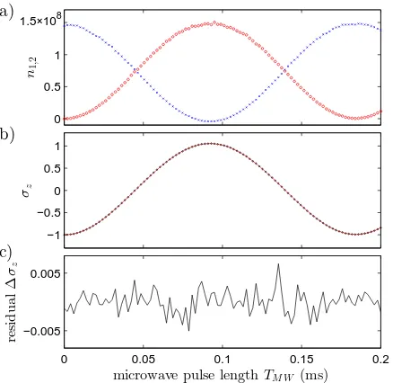
FIG. 7. Experimental detection of Rabi cycles. a) The popu-lations of both clock states_∣1,0_⟩(blue crosses) and_∣2,0_⟩(red circles) are measured as a function of microwave pulse dura-tion. b) Normalized population difference (circles) together with model function (solid line). c) The residuals indicate an oscillating noise amplitude. Each data point corresponds to a single experimental cycle.

ratio of the two signal strengths as a function of exter-nal field is extremal or, equivalently, when the ratio of signal strength to signal slope is identical for the two states. The static field that meets this condition depends on frequency shift and widths of both resonances. For equal resonance width, i.e., ∣B₊∣=∣B₋∣= ∣BRF∣/

√

2 and resonant field difference ∆B =−hω̵ /2gIµB, the optimal static field is found shifted from the resonance mean by ±1

2 √

∣BRF∣2+(∆B)2. As a consequence, signal strength

must be traded for maximal common mode noise suppres-sion. This can be improved by deliberately increasing the imbalance between the twoB_±-components, which shifts the optimal point closer to the resonance peaks.

Figure 6 b) shows experimental variances ⟨(∆σz)2⟩ for an equal superposition of clock states across the resonance for different experimental conditions. Away from resonance, noise increases due to diminishing sig-nal strength at constant detection noise (electronic and photon shot noise). For a small amount of deliberately introduced noise in the static field amplitude, the result-ing variance peaks near maximum signal strength and follows the expected behaviour. Generally, we achieve best performance near the point of stationary signal ra-tio closest to signal maximum. In our unshielded experi-ment, disabling synchronization with a 50 Hz line signal increases noise, which we attribute mainly to state prepa-ration noise in the fluctuating environment as this noise contribution remains fairly constant across the scan.

Measurement results of relative population difference σzfor driven Rabi cycles are shown in Fig.7. We observe

0 0.2 0.4 0.6 0.8 1

0 0.2 0.4 0.6 0.8 1

SUU= 3.6(9)×10−12 _V2_{s + 7.8(3)}

×10−8_V2_s/W

·P

light powerP (mW)

si

gn

al

n

oi

se

h

SU

U

i

(10

−

10V 2/

Hz

)

FIG. 8. Scaling of detection noise with probe power. The lin-ear dependence confirms shot noise limited performance for both probe lasers. Electronic noise is negligible in the typical operating range of a few hundred microwatts probe power. The shot noise scaling can be used to calibrate the electronic gaingel =U/Sz =2̵hωLU/∆P, relating output voltageU to photon flux or light power difference ∆P incident on the two detectors. For pure shot noise from the input light field of powerP and known quantum efficiency of the detectorη_<1 (electrons per photon), the electronic gain can be measured as gel =2

√_η̵

hωLζ⟨SU U⟩ /P ≈1.3×10−13V/Hz, assuming

quan-tum efficienyη=0.86 and an estimated noise power correction factorζ_≈0.5 due to aliasing.

high contrast fringes of Rabi frequency ΩRF =5.5 kHz,

which we model including a small exponential decay ac-counting for in-homogeneous microwave coupling across the atomic cloud. The residuals typically show noise variances on the order of 10−6 _{to 10−}5 _{varying across}

individual Rabi cycles. The noise is usually somewhat larger in the vicinity of zero crossings and increases with the number of cycles, indicating a contribution of state-preparation noise that scales with duration and power of the microwave driving.

C. Noise analysis

Analysis of different noise contributions to our mea-surements and distinction between technical and quan-tum noise can be based on parameter scaling.

Our balanced detector pair (Thorlabs PDB210A) is photon shot noise limited, confirmed by the linear de-pendence of noise power spectral densitySU U of the RF signal on light power in absence of atoms, see Fig.8. The detection electronics, including amplification and analog-to-digital conversion, introduce a small amount of elec-tronic noise that is negligible for the used light powers of typically a few hundred microwatts. In principle, the shot noise scaling allows for the determination of elec-tronic gaingel and thus linking the output amplitude to

0 5 10 15 20 0

0.5 1×10−4

pulse areaΩMWT(rad)

(

∆

σz

)

2 (∆σz)

2_{= 1.8}

×10−6_{+ 2.4}

×10−7_rad−2_(Ω MWT)2 (a)

0 0.2 0.4 0.6 0.8 1.0 1.2

0 0.5 1 1.5 2×1011

1.4×108

atom numbern

(

n

∆

σz

)

2

n

u

m

b

er

va

ri

a

n

ce

(n∆σz)2= 1.7×1010+ 9.4×10−6_n2

(n∆σz)2= 1.5×1010_{+ 3.7} ×10−6_n2

(b)

FIG. 9. Analysis of technical noise for (anti-)symmetric super-positions of the two clock states. a) State preparation noise is identified by driving the clock transition with odd multiples of π_/2 pulse areas and quantifying the quadratic scaling of vari-ance for 100 measurements. For aπ/2-pulse, we estimate an uncertainty contribution of ∆σz =

√

2.4×10−7⋅π/2≈0.08%.

b) Experimental data for variance of atom number difference show quadratic scaling with total atom number n for two experimental conditions. Signals were measured at constant magnetic field, fulfilling the RF resonance condition only for atoms withF₌2 (black squares). A small magnetic field shift introduced between the two probe pulses allows for resonant measurements on both states and reduces technical noise in-troduced by field fluctuations (blue circles). The model fits (solid lines) separate photon shot noise equivalent (dotted) and technical noise. Dashed lines indicate the estimated level of state preparation noise above photon shot noise.

a dedicated anti-aliasing filter, which leads to increased noise in the observed RF frequency band due to aliasing of photon shot noise.

Further noise stems from fluctuations in signal strength, caused by magnetic field fluctuations, as well as varying laser detunings, beam steering and imperfect cor-rection of light power fluctuations. Additional technical noise stems from the microwave driving and thus prepa-ration of the atomic state, and ultimately atomic shot noise. For further analysis, we generated (anti-)symmet-ric superpositions of the two clock states, i.e., ⟨ˆσz⟩= 0 and measured the variance of relative population differ-ence for different atom numbers and microwave dura-tions, see Fig. 9. The scaling with atom number shows that measurements at low atom number are limited by photon shot noise while measurements at high atom num-ber (n≈108_{) are dominated by technical noise}

contribu-tions on the order of ⟨(∆σz)2⟩=10−6−10−5, depending on the precise setting of static magnetic field strength. Our photon shot noise equivalent atom number resolu-tion is ∆n≈ √1.5×1010_{≈ 1.2}×₁₀5_{, i.e., ≈ 22dB above}

atomic shot noise for n= 108 _{atoms. The scaling with}

−10 0 10

p

h

as

e

2

ϕ1

,

2

(r

ad

)

a)

−150 −100 −50 0 50 100 150 200

−0.1 0 0.1

2

∆

ϕ1

,

2

(r

ad

)

half-wave plate angleϕ/2 (deg)

b)

FIG. 10. Dependence of 2ω-signal phases 2ϕ1,2 on half-wave

plate angle in the parallel setting (corresponding toϕ_/2). a) Experimental data are shown together with linear fits with slopes±(3.99±0.01)deg/deg, matching the expected value of ±4. b) The strong anti-correlation of residuals shows that the

dominant uncertainty stems from the wave-plate setting.

microwave duration shows a small contribution of state preparation noise.

D. State-to-quadrature mapping

We attribute a significant amount of technical noise in our measurements to the use of two independent probe beams, which do not probe the exact same volume. As a consequence, fluctuations in the position and shape of the atomic ensemble will translate into independent signal fluctuations. In addition, the lasers exhibit independent frequency and power fluctuations. While power fluctu-ations are co-measured and compensated for, small im-perfections like non-linearity and electronic noise in the detection system will degrade the performance. It is in principle possible to use a two-colour beam from a single laser, or phase and amplitude locked beams. Simultane-ous detection of both states will then achieve suppression of common mode noise. To distinguish the two signals, use can be made of the fact that the RF phase of the de-tected signal is adjustable and state-dependent, as rep-resented by the sign of the phaseϕin Eq.25-27.

−0.3 −0.1 0.1 0.3

ac

si

gn

al

U

(

t

)

(V)

0 0.5 1

p

ow

er

P1

+

P2

(m

W

)

a)

−0.5 0 0.5 1 1.5 2

0 0.05 0.1

IU

(

t

)

(V)

timet(ms)

0 0.05 0.1

QU

(

t

)

(V)

b)

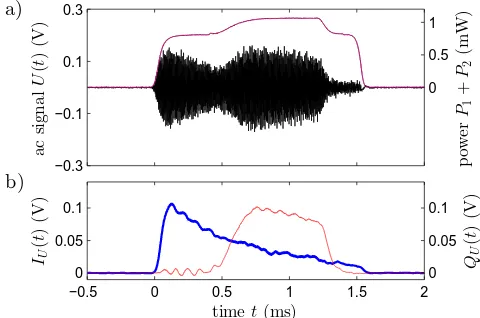
FIG. 11. Demonstration of state-to-quadrature mapping. Two probe pulses of different duration are sent through the atomic cloud with temporal overlap. a) The IQ-modulated RF signal from the atomic response (oscillating black curve) is shown together with total the light powerP1+P2(upper red

curve). The light pulse edges have been shaped to suppress ex-citation of Larmor precession in the effective field, which can occur at higher laser powers. b) The RF response is demod-ulated with 10 kHz bandwidth centred at 2ω₌360 kHz and separated into two orthogonal quadraturesIU(t)andQU(t). The light polarization was adjusted to obtain out-of-phase re-sponses from atoms inF₌1 (thick blue line) andF ₌2 (thin red line), i.e., by choosingϕ2−ϕ1≈π/2.

IV. CONCLUSIONS

We analysed and demonstrated dispersive detection of alkali atoms in radio-frequency dressed states. An exper-imentally simple polarimetric setup allows for low-noise measurements of atom numbers due to modulation of the atomic response at radio-frequencies. Linear bire-fringence measurements of driven Rabi-cycles between atomic clock states show technical noise on the cycle-phase on the order of 2 mrad. Future improvements may include the use of simultaneous probing of both states with two frequencies generated by a single, modulated laser. The ability to perform state to RF-quadrature mapping makes it possible to measure differential state population directly and potentially generate spin squeez-ing in the regime of strong light-matter couplsqueez-ing at suffi-cient optical density. The method can be used in various internal state atom interferometry experiments and may be extended to other dressed state schemes.

The datasets generated for this paper are accessible at [45] (Nottingham Research Data Management Repos-itory).

V. ACKNOWLEDGEMENTS

This work was funded by the EU (FP7-ICT-601180) and EPSRC (EP/M013294/1, EP/J015857/1). SJ was supported by the EU (FP7-PEOPLE-2012-ITN-317485).

We gratefully acknowledge useful discussions with I. Lesanovsky and thank K. Poulios for help with final cal-ibrations.

Appendix A: Dispersive measurement operators We consider a quasi one-dimensional situation with cross section A, light propagating along ez, and adopt a continuous medium, real space description of atomic and electromagnetic field operators as described in [35]. The electric field of a narrow-band light field of frequency ωL is described by Heisenberg operators for orthogo-nal polarizations j as ˆE = ∑j(Eˆj +Eˆj†), with ˆEj(z, t) = gej√1_2π∫ aˆk,jei(kz−ωLt)dk, whereg =√̵hωL/2ǫ0A scales

the field strength per photon, andejare unit polarization vectors. This can be written as

ˆ

Ej(z, t)=g[ˆaj(z, t)ej+ˆa†j(z, t)e∗j]. (A1)

Here, the creation and annihilation operators are de-fined as density amplitudes in position space, obeying [aˆi,ˆa†j]=δi,jδz(z)for orthogonal polarizations i, j, such that cˆa†_jˆaj describes photon flux. Different light polar-izations are conveniently described by introducing Stokes vector components that measure photon flux differences

⎛ ⎜⎜ ⎝

ˆ Sx

ˆ Sy

ˆ Sz

⎞ ⎟⎟ ⎠=

c 2

⎛ ⎜⎜ ⎝

ˆ a†

xˆax−ˆa†yˆay ˆ

a†_⤡ˆa_⤡−aˆ†_⤢ˆa_⤢ ˆ

a†₊ˆa₊−aˆ†₋ˆa₋ ⎞ ⎟⎟ ⎠=

c 2

⎛ ⎜⎜ ⎝

ˆ

a†₊ˆa₋+aˆ†₋ˆa₊ iˆa†₋ˆa₊−iˆa†₊ˆa₋

ˆ

a†₊ˆa₊−aˆ†₋ˆa₋ ⎞ ⎟⎟ ⎠, (A2)

where ˆa₊,− = (aˆx ∓iˆay)/ √

2, ˆa_⤡,⤢ = (±aˆx +ˆay)/ √

2, and ˆax,y describe circular σ±, linear ±45°, and horizon-tal/vertical polarizations, respectively. The Stokes vec-tor components obey commutation rules of angular mo-mentum, i.e., [Sˆx(t),Sˆy(t′)] =iδ(t−t′)Sˆz(t) and cyclic permutations [36]. In addition, we can measure the total photon flux of a beam of powerPas 2 ˆS0=c(ˆa†_iˆai+aˆ†_jˆaj)=

ˆ

P/̵hωL using any orthogonal pairei,j.

We are particularly interested in describing light-matter interaction in the off-resonant regime where ab-sorption of the fields can be neglected. Here, the interac-tion reduces to spin and polarizainterac-tion dependent disper-sion, governed by the frequency dependent polarizability tensor ˆα of the medium. The interaction energy can be expressed as a second-order perturbation with state-dependent dipole density ˆd, i.e., as a light-shift of the atomic ground states. The effective Hamiltonian can be stated as

ˆ

Heff =−∫ (Eˆ†αˆEˆ)Adz=∑ n ∫

ˆ E†_{Πgˆ dˆ}

ndˆ†nΠgˆ Eˆ ̵

h∆n Adz, (A3)

detunings ∆n=ωL−ωn. The projector ˆΠgreduces the de-scription of atomic dynamics to the relevant ground state manifold. For alkali atoms in their electronic ground state, the atomic dipole moment depends on the indi-vidual spin ˆFi, which we describe by a continuous op-erator function ˆf(z) for dimensionless spin per atom. The collective spin of N atoms distributed over any fi-nite lengthl with density ρ(z)is expressed as ∑Ni=1Fˆi= ∫lρ(z)ˆf(z)̵hAdz.

Using this description, the effective interaction Hamil-tonian for an atomic (sub)ensemble in one of the elec-tronic ground-state hyperfine manifolds (L=0, J= 1

2) of

certainF, can be expressed with irreducible tensor com-ponents. Following [35, 37–39] with some corrections, we use the expression

ˆ Heff=

g2

c ∫ L

0

ˆ

ΠF{2α(_F0)Sˆ0+2α( 1₎

F Sˆzfˆz (A4) +α(_F2)[2 ˆS0(fˆz2−fˆ

2_/

3)+Sˆ₊fˆ₋2+Sˆ₋fˆ₊2]}ΠFˆ ρAdz,

where ˆf_± = fˆx±ifˆy and ˆS± = Sˆx±iSˆy. This approxi-mate Hamiltonian depends on the strengthsα(_Fk) of the scalar, vector and tensor components of the polarizabil-ity,k=0,1,2, respectively. Considering only off-resonant driving of atoms to excited levels with electronic angu-lar momentumJ′, each component can have up to three contributions from transitions F → F′_{= F, F}±_{1, given} by

α(_F0)=AF−1

F + AFF+ AF+

1

F (A5)

α(_F1)=3 2[−A

F−1

F

F −

AF F

F(F+1)+ A F+1

F F+1]

α(_F2)=3 2[

AF−1

F F(2F−1)−

AF F F(F+1)+

AF+1

F

(F+1)(2F+3)].

The three contributions AF′

F for transitions from F to F′ are given by the respective detunings together with reduced dipole moments (which, by isotropy convention, sum up three orthogonal polarizations):

AF′ F =

1 3⋅ ∣⟨

J, F∣∣er∣∣J′, F′⟩∣2 ̵

h∆F,F′

=πǫ0c

3_ΓJ ′

∆F,F′ω3

J′

(2J′+1)(2F′+1){J J′ 1 F′ F I}

2

. (A6)

Here, we used a Wigner 6-j symbol and introduced decay rate ΓJ′ and frequencyω_J′ of spontaneous emission from

the excited J′ levels [34]. We assume AF′

F = 0 for non-existing transitions with undefined 6-j symbol, and for the mathematically indeterminate case where F = 0 in the denominator, the higher order terms areα(_F1,2)=0.

The effective Hamiltonian leads to Heisenberg equa-tions for the Stokes vector ˆS, given by(∂t+c∂z)Sˆ(z, t)= [_Sˆ_{(z, t),H}ˆ_eff]/ih̵_{. Neglecting retardation of light as it} propagates across short samples, i.e., ignoring the time

derivative, and using[ˆa(z, t),ˆa†(_z′_{, t}′_)]=δ(z−z′_{), results} in the following propagation equations for the Stokes pa-rameters:

∂Sˆx ∂z =

2g2_ρA

̵ hc [−α

(1)

F Sˆyfˆz+α(

2) F Sˆz(fˆ

2

↗−fˆ

2

↖)], (A7) ∂Sˆy

∂z = 2g2ρA

̵ hc [+α

(1₎

F Sˆxfˆz−α(

2₎

F Sˆz(fˆx2−fˆ

2

y)], (A8) ∂Sˆz

∂z = 2g2_ρA

̵ hc α

(2₎

F [+Sˆy(fˆ

2

x−fˆ

2

y)−Sˆx(fˆ

2

↗−fˆ

2

↖)], (A9)

where we used 45°rotated operators ˆf_↗,↖=(±fˆx+fˆy)/√2 for better clarity. The first two equations, as well as the two terms in the last expression, are each unitary equiv-alent under a 45°rotation about the z-axis. Terms con-taining ˆS0in the Hamiltonian, see Eq. (A4), cause global

phase shifts but do not change polarization. It can be seen that the set of equations describes rotations of the Stokes vector and that the rank-1 and rank-2 components of the polarizability are linked to circular and linear bire-fringence, respectively. Linear polarizations ˆSx,y experi-ence Faraday rotation about thez-axis, proportional to α(_F,J1)′ and longitudinal spin components ˆfz, i.e., atomic

orientation along z. Similarly, circular polarization ˆSz couples to ˆSx,y, proportional to α(_F2) and the alignment of transversal spin.

For the case of small optical phase shifts(≪1 rad), the induced rotations of the Stokes vector along the atomic ensemble will be small. If we also neglect backaction of light onto the atomic spin on the time scale of light traversion through the sample, we can approximate the right-hand sides of the propagation equations to be con-stant. As a result, the interaction with the atomic ensem-ble can be described using symmetric collective operators defined as

ˆ

Xx=∫ ρ(fˆx2−fˆ

2

y)̵h

2

Adz=∑ i

(_Fˆ2

x,i−Fˆ

2

y,i) (A10)

ˆ

Xy=∫ ρ(fˆ_↗2−fˆ_↖2)̵h2Adz=∑ i

(_Fˆ2

↗,i−Fˆ

2

↖,i) (A11) ˆ

Tz=∫ ρfˆzhAdz̵ =∑ i

ˆ

Fz,i, (A12)

with corresponding definitions for individual atomic op-erators ˆFj,i[40]. With these definitions and approxima-tions, the Stokes operators describing a probe beam after interaction with the atomic ensemble result from the in-tegration of propagation equations as

ˆ

S_x′ =Sˆx−g(

1)

F SˆyTˆz+g(

2)

F SˆzXˆy (A13) ˆ

S_y′ =Sˆy+g_F(1)SˆxTˆz−g(_F2)SˆzXˆx (A14) ˆ

S_z′ =Sˆz+g(

2)

F [SˆyXˆx−SˆxXˆy], (A15) with coupling constantsg_F(k) =2g2_α(k)

F /c̵hk+

1_{. The first}

For simplicity, we only consider strong classical probe light that is linearly polarized along the 45°-axes when it enters the atomic ensemble, i.e., ˆSx,z ≈0 and ˆSy ≈ Sy. In this case, Eqs. (A7) and (A9) and corresponding Eqs. (A13) and (A15) reduce to describing circular and linear birefringence independently. The resulting Fara-day rotation and resulting ellipticity reduce to

ˆ

S_x′ =Sˆx−g_F(1)SyTˆz ˆ

S_z′=Sˆz+g(

2₎

F SyXˆx, (A16) with signal strengths proportional to photon fluxSy. The link between these measurement operators and operators for the collective pseudo-spin formed from a two-level subspace is discussed in AppendixB.

Appendix B: Quantum mechanical interaction strength

In the following, we discuss our measurement scheme in the context of quantum noise and collective interaction strength between light and atoms, with the caveat that we assume the atomic state to be constant during the detection. Quantum mechanical back-action, dynamical phase evolution, as well as redistribution of population due to spontaneous emission into random directions are not included in our theoretical description. The effects on signal noise resulting from back-action and dynam-ical phase evolution are essentially caused by alternat-ing measurement of non-commutalternat-ing operators. In prin-ciple, they can be circumvented with stroboscopic mea-surements [41, 42] or combined meamea-surements on oppo-sitely oriented ensembles [43]. Redistribution of popu-lation generally leads to signal loss, but redistribution within or into the probed manifold will also generate ad-ditional signal noise.

It is useful to introduce canonical operators for the involved modes of light and atoms. The collective, two-level pseudo-spin is defined by ˆJj = 12∑iσˆj, which sums

individual Pauli operators. For large atom numbernand near-symmetric superpositions of the two states, we can define canonical, atomic operators ˆx,pˆ=Jˆy,z/ ⟨Jˆx⟩

1_/2

=

1

√

2n∑iσˆy,z. These quadratures obey [x,ˆ pˆ] ≈ i. The variance⟨(∆ˆp)2⟩₌ 1

2 describes the atomic shot noise of

level populations ˆn1,2, for which we can express

√ 2npˆ= ∑iσˆz=nˆ2−nˆ1 and thus⟨(∆(nˆ2−ˆn1))2⟩=n. Similarly,

we define operators for light as ˆy,qˆ=Sˆz,x/ ⟨Sˆy⟩

1/2

, which obey [yˆ(t),qˆ(t′)]≈iδ(t−t′) and correspond to quadra-tures of the mode that is orthogonally polarized to the classical input beam.

Based on the analysis described above, we can for-mulate measurement operators for the detected mode amplitudes. Separate interaction with hyperfine lev-els is accounted for using atomic projection operators

ˆ

ΠF =∑m∣F, m⟩⟨F, m∣in some basis. Including electronic noises(t)in the polarimeter signal, the real observables,

i.e., including both sides of the symmetric RF spectrum, are then given by

ˆ mF=

1 √

2∫ u

∗_[(s+g

elSˆz) (B1)

+gelg( 2) F Sy∑

i ˆ

ΠF,iFˆT_i Q_±FˆiΠF,iˆ ]dt+h.c.

We rewrite the sum by defining number-like operators ˆ

nF_l,m=∑i∣F, l⟩i⟨F, m∣i, and introduce the RF cycle inte-grated, atomic operator

ˆ QF F=

ω 2√2π∫

2π/ω

0 e

2i(ωt+ϕ)_FˆT_Q

±Fdtˆ +h.c. (B2)

to make the approximation

ˆ mF ≈∫

u∗+u √

2 (s+gel ˆ

Sz)dt (B3)

+gelg( 2)

F ∫ uS˜ ydt∑ l,m

⟨F, l∣QˆF F∣F, m⟩nˆFl,m,

This approximation makes use of the periodicityQ_±(t)= Q_±(t+2π/ω) and is valid for slowly varying envelopes, assumingω>>γ, T−1_{, which allows for piecewise}

integra-tion over RF cycles with approximately constant enve-lope.

We can scale the expression for our mode amplitudes to canonical operators

ˆ pF_l,m= nˆ

F l,m √

n, yˆu= 1 √

2∫ (u

∗_+u)√Sˆz Sy

dt. (B4)

For simplicity, we assume square laser pulses, i.e., con-stant photon fluxSy over the support of the mode func-tions. This allows us to introduce detection gaingdetand

interaction strengthκF as

gdet=gel √

Sy, κF =̵h2g(

2) F

√

nSy∫ udt.˜ (B5)

Using the coupling coefficients

cF_l,m=⟨F, l∣QˆF F∣F, m⟩ /̵h2, (B6)

the resulting mode amplitude can be expressed as

ˆ

mF =su+gdet ⎡⎢ ⎢⎢

⎢⎣yˆu+κF∑ l,m

cF_l,mpˆF_l,m ⎤ ⎥⎥ ⎥⎥ ⎦

, (B7)

where the contribution from electronic noise is given by su=∫ (u∗+u)sdt/

√ 2.

For atomic population in only one sublevel∣F, m⟩, the relevant quadrature operator will be ˆpF = pˆFm,m, with corresponding coefficient cF = cFm,m = ξF(m)h2(θ)/

√ 2. The expectation value of the measurement is then given by

Using the atomic operator variance

σ2_F=[⟨F, m∣Qˆ2_{F F}∣F, m⟩ − ⟨F, m∣QˆF F∣F, m⟩

2

] /̵h4, (B9)

and neglecting technical noise in detection gain or cou-pling strength, the variance of the measured mode am-plitude becomes

⟨(∆ ˆmF)2⟩=SU Uel +g

2

det[ ⟨(∆ˆyu)2⟩ (B10) +κ2_F(⟨√pˆF⟩

nσ

2

F+c

2

F⟨(∆ˆpF)2⟩)],

where we introduced the power spectral density Sel

U U = ⟨(∆su)2⟩of electronic noise in the detected voltageU(t) and made use of the fact that the operator ˆQF F does not change the hyperfine level.

Atomic quantum noise will become relevant in the regime of strong interaction (κF ⋅ O(F2) ⪆ 1). For a coherent input state, the light noise is ⟨(∆ˆyu)2⟩ = 12.

For a symmetric superposition of one state in each hy-perfine manifold, i.e., a coherent spin state, the anti-correlated atomic operators each have expectation val-ues ⟨pˆF⟩ = √n/2 and variances ⟨(∆ˆpF)2⟩ = 1₄. Con-sidering different coupling strengths and detection gains, appropriate weighting of the two mode amplitudes ˆm1,2

will lead to some effective coupling strength ˜κc˜and al-low for measurements of ˆp=(pˆ2−pˆ1)/

√

2 with variance ⟨(∆ˆp)2⟩₌ 1

2. We have to note, however, that the clock

states∣1,0⟩and ∣2,0⟩ used here are generally not eigen-states of ˆQF F, which leads to additional atomic noise contributions according to Eq.B10. In the parallel set-ting under the resonance condition θ= π/2, the atomic operator is ˆQF F =(Fˆy2−Fˆz2)/

√

2, providing a true QND measurement of its eigenstate ∣1,0⟩ with c1 =1/

√ 2 and σ2

1=0. Resonant measurement of∣2,0⟩leads toc2=3/ √

2 and σ2

2 = 3/2. For general states ∣F, Fz=0⟩ of bosonic atoms, the additional noise can be calculated from the variance

⟨(∆(Fˆy2−Fˆ

2

z))

2

⟩= (F−1)F(F+1)(F+2)

8 h̵

4

. (B11)

The resulting noise in the combined measurement will depend on the chosen coupling strengths, detection gains and corresponding signal weighting. In principle, a weak measurement of ˆn2 is sufficient to gain information on

the total atom number n when combined with a strong measurement of ˆn1. Therefore, the optimal

measure-ment strategy and achievable degree of measuremeasure-ment in-duced spin squeezing depends on the uncertainty of total

atom number. This analysis together with consideration of back-action, dynamical phase evolution, spontaneous emission, and breakdown of other approximations made throughout the above derivations is beyond the scope of this paper.

From our measurement data we infer operation in the weak coupling regime for the given optical depth. From the ratio(κ˜˜c)2_≈n/(_ζ⋅_1.5×₁₀10)_{of assumed atomic shot}

noise to (aliasing corrected, ζ ≈ 0.5) photon shot noise equivalent, neglecting electronic noise as well as detector inefficiency, we estimate an effective interaction strength on the order of ˜κ˜c ≳0.14 for the measurement of ˆpfor an experimentally somewhat uncertain atom numbern≈ 1.5×108_{, which we can compare to the prediction. For}

long pulses, the interaction is limited by atomic decay. The maximal effective interaction time resulting from an infinite exponential mode function given in Eq.28using T =∞, is_∫ udt˜ =√2/γ. Still assuming constant atomic signal, we can express an upper bound to the coupling strength as

κF = α(_F2)

αJ′ ΓJ ′ λ

2

4πA √

λ hc

nP

2 ∫ udt˜ (B12)

≤√χ⋅ΓJ′λ 2

4π √

λ hc

n

A. (B13)

This defines the detuning dependent figure of meritχ= (α(_F2)/αJ′)2P/Aγ shown in Fig. 2 c), which determines

the maximal signal-to-noise power ratio at fixed optical depth.

For our Gaussian atomic density distribution with standard deviation σ0 ≳ 1.2 mm and mode matched

probe beams, the effective interaction area isA=4πσ2 0≳

18 mm2_{[44]. With probe detunings and observed, power}

dependent decay rates for F = 1 (∆1,1 ≈ 240 MHz,

γ≈900 s−1 _at

P =540µW) andF=2 (∆2,1≈400 MHz,

γ≈350 s−1_at

P=120µW), we predict maximal coupling strengths ofκ1c1≲0.21 andκ2c2≲0.35 forn=1.5×108

atoms, using long pulses and complete decay. Here, we use shorter pulses, with only 1 ms for the measurement of ˆp2. This minimizes expansion of the falling cloud as

well as an error on the subsequent measurement of ˆp1due

to the increase of population inF =1 from spontaneous emission. The short pulse duration reduces the theo-retical coupling strength to κ2c2≲0.14. The estimated

effective strength compares well with the predicted val-ues. Further increase of coupling strength and entering the strong coupling regime, especially for QND measure-ments with minimal atomic loss, requires an increase of optical depth.

[1] B. M. Garraway and H. Perrin, J. Phys. B: At. Mol. Opt. Phys.49172001 (2016).

[2] T. Schumm, S. Hofferberth, L. M. Andersson, S. Wil-dermuth, S. Groth, I. Bar-Joseph, J.

Schmied-mayer and P. Kr¨uger, Nature Physics 1 57 (2005),

arXiv:quant-ph/0507047.

Journal of Physics B: Atomic, Molecular and Optical Physics391055 (2006),arXiv:quant-ph/0512061.

[4] G. A. Sinuco-Le´on and B. M. Garraway, New Journal of Physics17, 053037 (2015).

[5] T. Fernholz, R. Gerritsma, P. Kr¨uger and R. J. C. Spreeuw, Physical Review A 75 063406 (2007),arXiv:physics/0512017[physics.atom-ph].

[6] I. Lesanovsky and W. von Klitzing, Physical Review Let-ters99, 083001 (2007), arXiv:cond-mat/0612213 [cond-mat.quant-gas].

[7] B. E. Sherlock, M. Gildemeister, E. Owen, E. Nugent and C. J. Foot, Physical Review A 83,043408 (2011),

arXiv:1102.2895[cond-mat.quant-gas].

[8] P. Navez, S. Pandey, H. Mas, K. Poulios, T. Fernholz and W. von Klitzing, New Journal of Physics18075014 (2016),arXiv:1604.01212 [quant-ph].

[9] Y. Colombe, E. Knyazchyan, O. Morizot, B. Mercier, V. Lorent and H. Perrin, Europhysics Letters 67, 593 (2004),arXiv:quant-ph/0403006.

[10] S. Hofferberth, I. Lesanovsky, B. Fischer, J. Verdu and J. Schmiedmayer, Nature Physics 2, 710 (2006),

arXiv:quant-ph/0608228.

[11] E. Bentine, T. L. Harte, K. Luksch, A. J. Barker, J. Mur-Petit, B. Yuen and C. J. Foot, Journal of Physics B: Atomic, Molecular and Optical Physics 50, 094002 (2017),arXiv:1701.05819 [cond-mat.quant-gas].

[12] R. Stevenson, M. R. Hush, T. Bishop, I. Lesanovsky and T. Fernholz, Physical Review Letters115, 163001 (2015),

arXiv:1504.05530[physics.atom-ph].

[13] T. Fernholz, H. Krauter, K. Jensen, J. F. Sherson, A. S. Sørensen and E. S. Polzik, Physical Review Let-ters101, 073601 (2008),arXiv:0802.2876[quant-ph].

[14] K. Jensen, W. Wasilewski, H. Krauter, T. Fernholz, B. M. Nielsen, M. Owari, M. B. Plenio, A. Serafini, M. M. Wolf and E. S. Polzik, Nature Physics7, 13 (2011),

arXiv:1002.1920[quant-ph].

[15] H. Krauter, D. Salart, C. A. Muschik, J. M. Petersen, H. Shen, T. Fernholz and E. S. Polzik, Nature Physics9, 400 (2013),arXiv:1212.6746[quant-ph].

[16] W. M. Itano, J. C. Bergquist, J. J. Bollinger, J. M. Gilli-gan, D. J. Heinzen, F. L. Moore, M. G. Raizen and D. J. Wineland, Physical Review A47, 3554 (1993).

[17] D. Budker and M. Romalis, Nature Physics3, 227 (2007),

arXiv:physics/0611246[physics.atom-ph].

[18] A. D. Ludlow, M. M. Boyd, J. Ye, E. Peik and P. Schmidt, Reviews of Modern Physics87, 637 (2015),

arXiv:1407.3493[physics.atom-ph].

[19] A. D. Cronin, J. Schmiedmayer and D. E. Pritchard, Reviews of Modern Physics 81, 1051 (2009),

arXiv:0712.3703[quant-ph].

[20] C. M. Caves, Physical Review D23, 1693 (1981).

[21] D. J. Wineland, J. J. Bollinger, W. M. Itano and D. J. Heinzen, Physical Review A50, 67 (1994).

[22] L. Pezz`e, A. Smerzi, M. K. Oberthaler, R. Schmied and P. Treutlein (2016),arXiv:1609.01609[quant-ph].

[23] D. Heine, W. Rohringer, D. Fischer, M. Wilzbach, T. Raub, S. Loziczky, X. Liu, S. Groth, B. Hessmo and J. Schmiedmayer, New Journal of Physics 12, 095005 (2010),arXiv:1002.1573 [cond-mat.quant-gas].

[24] G. W. Biedermann, X. Wu, L. Deslauriers, K. Takase and M. A. Kasevich, Optics Letters34, 347 (2009).

[25] K. C. Cox, G. P. Greve, J. M. Weiner and J. K. Thompson, Physical Review Letters116, 1 (2016),

arXiv:1512.02150[physics.atom-ph].

[26] O. Hosten, N. J. Engelsen, R. Krishnakumar and M. A.Kasevich, Nature529, 505 (2016).

[27] S. Franke-Arnold, M. Arndt and A. Zeilinger, Journal of Physics B: Atomic, Molecular and Optical Physics 34, 2527 (2001).

[28] T. Morgan, Th. Busch and T. Fernholz (2014),

arXiv:1405.2534[quant-ph].

[29] T. L. Harte, E. Bentine, K. Luksch, A. J. Barker, D. Try-pogeorgos, B. Yuen and C. J. Foot, Physical Review A

97, 013616 (2018), arXiv:1706.01491 [cond-mat.quant-gas].

[30] C. Foot, private communication.

[31] C. Cohen-Tannoudji, J. Dupont-Roc and G. Grynberg, Atom-Photon Interactions: Basic Processes and Applica-tions (Wiley-VCH Verlag GmbH), Weinheim, Germany (1998).

[32] F. Bloch and A. Siegert, Physical Review57, 522 (1940).

[33] W. Petrich, M. H. Anderson, J. R. Ensher and E. A. Cor-nell, Journal of the Optical Society of America B11, 1332 (1994).

[34] D. A. Steck, Rubidium 87 D Line Data, available on-line athttp://steck.us/alkalidata(revision 2.1.5, 13 Jan-uary2015).

[35] B. Julsgaard, Entanglement and Quantum Interaction-swith Macroscopic Gas Samples, Ph.D. thesis, Depart-ment of Physics and Astronomy, University of Aarhus, Denmark (2003).

[36] Note thatδ₍t_{) =}c⋅δz(z=ct).

[37] D. V. Kupriyanov, O. S. Mishina, I. M. Sokolov, B. Julsgaard and E. S. Polzik, Physical Review A - Atomic, Molecular, and Optical Physics 71 (2005),

arXiv:quant-ph/0411083.

[38] J. M. Geremia, J. K. Stockton and H. Mabuchi, Physical Review A73, 042112 (2006),arXiv:quant-ph/0501033.

[39] S. R. de Echaniz, M. Koschorreck, M. Napolitano, M. Kubasik and M. W. Mitchell, Physical Review A77, 032316 (2008),arXiv:0712.0256[quant-ph].

[40] In the subspace forF₌1, these operators can be scaled to follow commutation rules of a collective pseudo-spin, see ref. [39].

[41] G. Vasilakis, V. Shah and M. V. Romalis, Physical Re-view Letters106(2011),arXiv:1011.2682 [quant-ph].

[42] G. Vasilakis, H. Shen, K. Jensen, M. Balabas, D. Salart, B. Chen and E. S. Polzik, Nature Physics11, 389 (2015),

arXiv:1411.6289[quant-ph].

[43] B. Julsgaard, A. Kozhekin and E. S. Polzik, Nature413, 400 (2001),arXiv:quant-ph/0106057.

[44] The quantum mechanical interaction strength and thus signal-to-noise ratio is highest for mode matched beams and is reduced for other profiles or beam irregularities. However, a non-flattop beam shape will interact with the corresponding spatial mode of the atomic ensemble, re-ducing the effective number of atoms, which becomes rel-evant for other than coherent spin states.