Quantifying the impact of variability in railway bridge asset management

Quantifying the Impact of Variability in Railway Bridge Asset

Management

P. C. Yianni

Asset Management Advisory, Jacobs UK,

Wokingham, Berkshire, RG41 5TU, United Kingdom.

L. C. Neves, D. Rama, J. D Andrews

Resilience Engineering Research Group, Faculty of Engineering,

University of Nottingham, University Park, Nottingham, NG7 2RD, United Kingdom.

N. Tedstone, R. Dean

Network Rail, The Quadrant:MK, Elder Gate, Milton Keynes, Buckinghamshire, MK9 1EN, United Kingdom.

ABSTRACT: Bridge asset management is often a challenging and complicated task due to the diversity, multitude and variation of bridge configurations. Much research has been carried out in the field of asset management which has resulted in a wealth of models to help with the decision making process. However, often these models oversimplify the process, resulting in a decision making tool that trivialises the complexity of the decisions. The purpose of this study was to ascertain what the main sources of variability are in the process and then quantify the impact of them in terms of the Whole Life-Cycle Cost (WLCC). The study focuses on human-induced variability to ensure the results are directly influenceable by bridge portfolio managers. The sources of variability identified include misdiagnoses of defects as well as imperfect repairs and variability in costs, all of which are aspects that bridge portfolio managers are exposed to. The sources of variability are quantified and then incorporated into an existing railway bridge WLCC model, established in a previous study, which uses a flexible Petri-Net (PN) approach which is able to incorporate the complex logic and probabilistic aspects. The model itself is able to replicate some of the more complicated decisions which have to be made in bridge asset management, especially those which influence the decisions around rehabilitation. The resulting model, enhanced with the probabilistic variability, is able to reveal the impact of variability on the asset condition, WLCC and even understand where operational complexities are occurring within the system. Incorporating human-induced variability into any model will inevitably increase the financial and operational burden predicted by the model, however, recognising and modelling these aspects is a crucial step in providing bridge portfolio managers a more robust and accurate decision making tool which can more accurately replicate the real world system.

1 INTRODUCTION

The rail infrastructure in the UK is key to com-merce, enabling the mobilisation of both people and materials. Management of the railway can be difficult due to, firstly, its extended heritage re-sulting in many legacy systems, assets and tech-niques (Network Rail 2010d). Secondly, the in-frastructure utilises diverse asset groups covering signalling and control groups, electrification and power management systems, structures and struc-tural support groups and the track itself. Finally,

due to the increasing demand of the infrastruc-ture, especially when considering the step changes with the introduction of European Train Control System (ETCS) (Technical Strategy Leadership Group (TSLG) 2012).

man-aging bridges over their life-cycle.

There have been a number of studies that have modelled bridge asset management, each using dif-ferent modelling methods and assumptions (Fran-gopol, Kallen, & van Noortwijk 2004, Miyamoto, Kawamura, & Nakamura 2000, Morcous, Rivard, & Hanna 2002). However, what often occurs dur-ing the creation of these models is that the system, and the decision making process, is oversimplified in the model. This often means that the resulting model, although accurate in its replication of indi-vidual processes, does not consider the overall sys-tem complexity. Because of this, the usefulness of the model is often limited from the perspective of a bridge portfolio manager. One of the major factors often overlooked when modelling bridge portfolio management is that it relies on human recogni-tion, identification and decisions, which are prone to error and variability. Trying to incorporate this human-induced variability into a bridge manage-ment model would help improve the usefulness of the model outputs to bridge portfolio managers.

2 LITERATURE REVIEW

To be able to analyse variability within a system, a great deal needs to be understood about the sys-tem and the decisions which are made within that system. Some of these decisions will be governed by industry standards and organisational policy, but other decisions will rely on human interpre-tation and decision making. Madanat 1993 and Ben-Akiva, Humplick, Madanat, & Ramaswamy 1993 identify two fundamental sources of variabil-ity within models: 1) the certainty of the cur-rent asset condition and 2) the forward prediction of the asset condition. The studies both identify that the variability in asset condition can arise from measurement errors, defect diagnosis errors and data input errors, amongst others. The au-thors state that variability of inspections had not been incorporated into any bridge maintenance and rehabilitation model until then. Misdiagno-sis during an inspection can lead to major con-sequences with regards to incorrect maintenance being scheduled. The authors argue that policies are designed to recommend a suitable maintenance action which means that a misdiagnosis can only lead to scheduling a maintenance action that is less suitable. The studies both assume that the condi-tion reported by the inspeccondi-tions can contain errors. The reported condition is only probabilistically re-lated to the actual condition of the asset. The au-thors perform a parametric study to ascertain the effect of variability on the final model outputs. The results of the study are that as the standard devia-tion widens, which represents a greater amount of variability, the higher the WLCC of the asset over its lifetime. Although this study parametrised and

quantitated the variability, the WLCC could have been considered in more detail.

Phares, Washer, Rolander, Graybeal, & Moore 2004 and Moore, Phares, Graybeal, Rolander, & Washer 2001 investigated the variability in inspec-tion results carried out on highway bridges. For this study, they collaborated with 49 bridge inspec-tors who had been trained to the National Bridge Inspection Standards (NBIS), which is the stan-dard in the USA. The inspectors were asked to carry out 10 different field tests across a range of different types of bridges. The asset condi-tion reported by each of the inspectors was com-pared against the Federal Highway Administra-tion (FHWA) Non-destructive EvaluaAdministra-tion Valida-tion Center (NDEVC). The NDEVC condiValida-tion was used as the known/true asset condition and each of the inspectors reported condition scores was com-pared against it. The results showed that 78% of the condition scores reported by the inspectors were correct at a 95% probability. The authors conclude that the vast majority of condition rat-ings (95%) will be within two condition scores of the true condition, using the NBIS condition scale. This study is significant in quantifying the variabil-ity of visual inspections.

Neves & Frangopol 2010 analysed the variabil-ity of inspections on bridge assets. The analysis showed that there are a number of factors which influence the quality of inspections including: the experience of the inspector, the ease of access of the asset elements, the topology/configuration of the bridge and the types of defects. Using these fac-tors, a probability of misdiagnosis was calculated. The results showed that a good quality inspection only has a 5% probability of misdiagnosis whereas a poor quality inspection produces a 40% proba-bility of being misdiagnosed.

3 NR BRIDGE MANAGEMENT POLICIES 3.1 Condition States

Network Rail (NR), the UK’s largest railway owner and operator, separate each of their bridges into individual elements, which are each inspected and scored. The condition scoring system used is a 2-dimensional, discrete condition system known as the Severity Extent Rating (SevEx). One axis con-tains the type of defect and the other axis de-tails the extent of the defect. The SevEx matri-ces vary depending on the material composition of the element. Concrete bridges are used in this study as the exemplar material type as they are be-coming the de facto standard for new bridges and therefore their management is becoming increas-ingly more important. The SevEx matrix for con-crete elements ranges from A1, an “as new” condi-tion to G6, which refers to a permanent structural defect. The majority of defects within the con-crete SevEx matrix relate to cracking and spalling. When the elements get inspected, the SevEx dition is recorded for each one. The historical con-dition recordings are all stored within a database, which will be discussed on Section 4.

3.2 Inspection Policy

There are two types of inspection which are stan-dard within the railway industry for bridge as-sets: 1) visual examinations, which occur yearly to ensure asset safety and 2) detailed examinations which are scheduled according to the asset con-dition. During detailed examinations the element conditions are recorded; detailed examinations are the focus of this study.

NR determine the inspection interval based on the condition of the asset (Network Rail 2010b). Assets in good condition (condition states A1, B2-B5, C2-C3 and D2) are inspected every 12 years, those in medium condition (B6, C4-C6, D3-D5, E2-E5 and F2-F3) are inspected every 6 years and assets in poor condition (D6, E6, F4-F6 and G2-G6) are inspected every 3 years. This sys-tem was developed using a risk based approach and has been back-converted to the SevEx condi-tion matrix for ease of comparison in this study.

3.3 Maintenance Actions

NR determine the appropriate maintenance action based on the condition of the asset (Network Rail 2012a). There are three main maintenance types which are performed: 1) Minor repairs, which are carried out on elements in condition states B2-B4, C2-C3 and D2, 2) Major repairs, which are car-ried out on elements in condition states B5-B6, C4-C6, D3-D5, E2-E4 and F2-F3 and 3) Replace-ments, which are carried out on elements in

con-dition states D6, E5-E6, F4-F6 and G2-G6. The threshold for a replacement to be carried out is set by the Basic Safety Limit (BSL) within the in-dustry standards for safety (Network Rail 2010a). This process has also been developed using a risk based approach, and back-converted to the SevEx condition matrix for ease of incorporation in this study.

4 DATA SOURCE

A variety of data sources were used in this study, ranging from asset registers, Civil Asset Regis-ter and Reporting System (CARRS), to inspection databases, Structure Condition Monitoring Index (SCMI), and work order databases, MONITOR and the Cost Analysis Framework (CAF).

As mentioned in Section 3.1, bridge assets are split into their constituent elements via a defined hierarchy (Network Rail 2012b). There is a total of 25,949 bridge assets within the dataset. The to-tal number of minor elements in the dataset is 563,150. The total number of inspections on mi-nor elements is 1,397,748 within the dataset.

Concrete bridges were chosen as the exemplar material type for this analysis. There are 4,434 concrete bridges in the dataset. The main girder elements were chosen as the exemplar element as they are often the Primary Load Bearing Ele-ment of concrete bridges. In the dataset there are 407,708 inspections of concrete main girders.

5 VARIABILITY OF INSPECTIONS AND INTERVENTIONS

5.1 Variability of Inspections

Detailed examinations are carried out by trained inspectors who assess each element in detail. Most railway bridge assets in the UK are inspected in person, as oppose to using remote condition equip-ment, and there are differences between inspectors in both their physical recognition of defects (i.e. differences in eyesight) even if their technical train-ing and competence is the same.

Detailed examinations are carried out within touching distance of the element (Network Rail 2010c). Each of the elements has their condition recorded according to the SevEx scale and is often accompanied by a photograph. A senior inspector will review the recorded conditions and the pho-tographs; these members of staff often have risen to the position with many years experience and so their identification of defects and the severity of the defects is good, but not infallible.

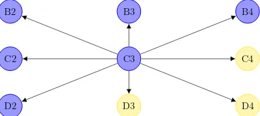
Washer 2001, studied the variability of defect iden-tification on bridge assets. The results were that the inspectors were correct to within two condi-tion states. The condicondi-tion scale used in this study was linear whereas the condition scale used by NR is the 2-Dimensional SevEx scale. Transposing the results found by the authors to the SevEx scale results in an equivalent variability of±1 condition state. Therefore, for a particular condition state, there may be up to 8 surrounding states within the ±1 condition range, as seen in Figure 1.

B2 B3 B4

C2 C3 C4

D2 D3 D4

Figure 1: Variability associated with a reported condition score.

In the example shown in Figure 1, a C3 con-dition is reported by the inspector as the element condition. However, due to variability of the exam-ination process, the C3 being reported could relate to any of the condition states shown. The mainte-nance action recommended for an element in a C3 condition would be a minor repair. However, the maintenance action which is recommended for an element in condition states C4, D3 and D4 would be a major repair. Therefore, the consequence of an erroneous identification is that it could lead to the wrong type of maintenance being scheduled.

Table 1 shows the results of the analysis carried out on the SevEx condition matrix to identify the probability of each condition state leading to the wrong type of maintenance action being scheduled, using the±1 variability. Where a condition state is on the border of two different maintenance actions, the probability of a misdiagnosis leading to an er-roneous maintenance action is higher. Condition states that are not near borders are not as crit-ical because an erroneous condition identification would still result in the same maintenance action. On average, using the±1 variability range, main-tenance actions are scheduled correctly 72% of the time.

5.2 Imperfect Interventions

Often bridge management models either do not consider maintenance as an explicit action or as-sume that maintenance is perfect (i.e. maintenance improves the condition to a predefined condition state, often the “as new” or A1 condition) Mor-cous & Lounis 2006, van Noortwijk & Klatter 2004, Le & Andrews 2013. Although this assump-tion is an oversimplificaassump-tion of the system, to dis-pense with the assumption requires an

evidence-Table 1: Probabilities of scheduling the correct maintenance

action when considering inspection variability of±1

condi-tion state.

State B2 B3 B4 B5 B6

Probability 1.00 0.80 0.40 0.80 1.00

State C2 C3 C4 C5 C6

Probability 0.80 0.63 0.63 0.75 0.80

State D2 D3 D4 D5 D6

Probability 0.40 0.63 0.75 0.63 0.40

State E2 E3 E4 E5 E6

Probability 0.80 0.75 0.63 0.63 0.80

State F2 F3 F4 F5 F6

Probability 0.60 0.50 0.63 0.88 1.00

State G2 G3 G4 G5 G6

Probability 0.33 0.60 0.80 1.00 1.00

based approach. Therefore, data analysis was car-ried out using historical maintenance and inspec-tion records to determine the variability in the con-dition uplift after an intervention.

The inspection data available for this study in-cludes both deterioration and condition uplift. In the previous section it was determined that there is some variability regarding the accuracy and re-peatability of element inspections. To ensure this analysis only considers situations where there has been an uplift in condition due to an intervention, rather than due to any variability within the in-spection procedure, only element condition uplifts of more than one condition state were considered. The exemplar element used throughout this study is the concrete main girder, on which this analy-sis was performed. The total number of element inspections which was used for this analysis was 49,300.

The analysis results are presented in Table 2 where it can be seen that interventions which re-turn the element condition to A1, the “as new” state, which represents a “perfect repair”, only ac-counts for 43% of the condition uplifts. This is in stark contrast to what most bridge management models assume as the result shows that perfect re-pairs do not even occur in the majority of occur-rences. The next most populous condition state is B3, which accounts for 29% of all condition uplifts following an intervention.

Table 2: Probabilities of resulting condition states following an intervention.

State A1 B2 B3 B4 C2 C3 D2

Percent 43% 6.5% 29% 10% 0.4% 11% 0.1%

5.3 Summary

maintenance actions are appropriate for the con-dition of the element. In adcon-dition to this, an anal-ysis has been carried out on the condition uplift following an intervention. This demonstrated that a “perfect repair” only occurs 43% of the time, which is in stark contrast to the assumption made by many other bridge management models that all interventions result in perfect repairs. These as-pects will now be incorporated into an existing WLCC model to quantify the impact that these sources of variability have on the overall system.

6 WLCC PN MODEL

PNs, created by Petri 1962, have been gaining in popularity in modelling systems within the com-munications, manufacturing and engineering sec-tors (British Standards Institution 2012). An exist-ing WLCC model will be used in this study which uses the PN approach (Yianni, Rama, Neves, An-drews, & Castlo 2016). The advantage that the PN approach brings to this type of study is that the logic and probabilistic elements can be more easily incorporated than in other modelling approaches, as demonstrated by Andrews 2013. The more ad-vanced features of the model use the Coloured Petri-Net (CPN) techniques introduced by Jensen 1997.

The PN WLCC model uses a number of differ-ent modules which each mimic a differdiffer-ent aspect of bridge management, ranging from the deterio-ration module to the inspection and maintenance modules. Each of these has been designed and calibrated using a combination of historical data, expert judgement and industry standard policies. The details which follow in this section are specif-ically in relation to the modules of the PN model which are affected by the variability discussed within this study. The model itself is simulated using a Monte Carlo (MC) approach and the out-puts are aggregated to provide a yearly overview, which gives an insight into the overall system be-haviour. The full model, and details of all the in-dividual modules, are given in detail in Yianni, Rama, Neves, Andrews, & Castlo 2016.

6.1 Maintenance Action Module

The maintenance action module simulates the events immediate after an inspection, during which the appropriate maintenance action is decided upon. As detailed in Section 5.1, the variability of inspections can lead to incorrect maintenance ac-tions being scheduled. The probability of a defect misdiagnosis occurring is 28%.

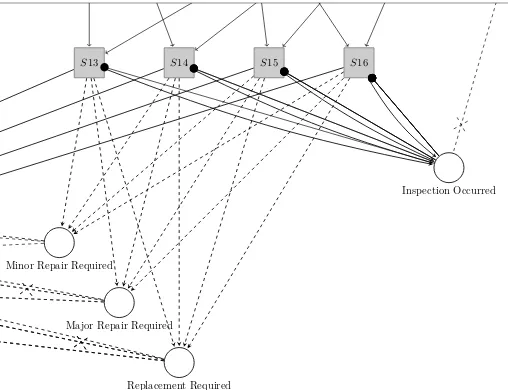
Within the statistical model, each of the PN transitions have been enhanced with probabilistic capabilities and have had the probabilities from Table 1 embedded within them. These are shown

in Figure 2 by transitionsS13−S16. The effect of

this is that there is a probabilistic outcome for the maintenance actions, calibrated with the probabil-ities calculated in Table 1. This ensures that the same probability of an incorrect maintenance ac-tion being scheduled in the real-world system is mirrored within the statistical model.

A1

B2 B3

C2 C3

Pending Condition

Condition Determined Condition Change

T1 T2

T3

T4

T5 T6 T7

T8

T10 T9

A1

B2 B3

C2 C3

Minor Repair Required

Major Repair Required

Replacement Required Intervention Planned

Between Inspection

During Inspection

Inspection Occurred

S13 S14 S15 S16

T11

T12

Between Intervention

Intervention Commences

T17 T18

Figure 2: The maintenance action module captures the vari-ability in the outcome of the inspection procedure.

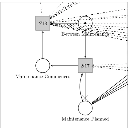
6.2 Intervention Module

The intervention module is activated once a main-tenance action has been determined, following an inspection. The module is modelled on mainte-nance teams arriving on site to carry out an in-tervention and performing an initial investigation to ascertain if the condition of the element and the maintenance action are compatible. The tran-sition, markedS18, contains a complex CPN guard

which checks the type of maintenance action which has been scheduled against the condition of the el-ement. This allows it to determine if the correct maintenance action has been scheduled or not. The variability in inspection, which this model is en-hanced with, affects both the maintenance action module and the intervention module.

The intervention module has been embedded with the results of the imperfect repair analysis, as seen in Section 5.2. In the model, there is a probabilistic output to the condition module which means that the condition uplift following an inter-vention is calibrated to the probabilities seen in Table 2. This ensures that the condition uplift fol-lows the same profile as that seen in the real world system.

A1

B2 B3

C2 C3

Pending Condition

Condition Determined Condition Change

T1 T2

T3

T4

T5 T6 T7

T8

T10

T9

A1

B2 B3

C2 C3

Minor Repairs

Major Repairs

Minor Repair Required

Major Repair Required

Replacement Required Maintenance Planned

Between Inspection

During Inspection

Inspection Occurred

T13 T14 T15 T16

T11

T12

Between Maintenance

Maintenance Commences

S17

S18

Petri-Net for a Minor Element: Main External Girder (MGE), Concrete (C). All advanced transitions functions are represented with dashed arcs. WhereD/Prepresents a decision making

probability transition that uses a random number to determine which probability the token is placed into e.g. (10%,80%,10%) if one of the inputs is designed to inhibit then the other op-tions increase proportionately i.e. if the first 10% was inhibited then the options would become 80%+(80/90*10) = 88.89% and 10%+(10/90*10) = 11.11%;D/Mrepresents a transition

func-tion where a decision is based on marking, for instance it may determine the worst condition from the Sub-Minor Element con-ditions and places a token in the relevant place;Rrepresents a

transition that is designed to reset a place or multiple places.

Transition Delay Type D/M D/P R

T1 Stochastic No No No

T2 Stochastic No No No

T3 Stochastic No No No

T4 Stochastic No No No

T5 Stochastic No No No

T6 Stochastic No No No

T7 Stochastic No No No

T8 Stochastic No No No

T9 Instant No No Yes

T10 Instant Yes No Yes

T11 Conditional Yes No No

T12 Small Delay (ε) No No Yes

T13 Instant Yes Yes No

T14 Instant Yes Yes No

T15 Instant Yes Yes No

T16 Instant Yes Yes No

T17 Conditional Yes No Yes

T18 Conditional Yes Yes Yes

Figure 3: The intervention module is affected by variabil-ity of inspections, variable intervention costs and imperfect repairs.

the enhanced scenario, which does consider the human-induced variability, using the results from the previous sections. This allows an effective com-parison to quantify the effect of variability on the WLCC of bridges. To simulate an entire bridge asset, an equal number of PN tokens to bridge el-ements would be entered into the model. For illus-trative clarity, the outputs shown in this section were calculated based on a simulation with a sin-gle concrete girder element, the exemplar element used throughout this study. The model is simu-lated using a MC simulation approach over a 100 year timespan.

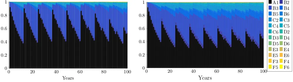
Figure 4 shows the model output which aggre-gates the element condition states. It can be seen in Figure 4(a), the control scenario, which does not consider imperfect repairs, that the element spends the majority of the simulation period, ~60%, in condition state A1. This is because the element experiences repeated condition uplifts, following “perfect repairs”, to the A1 “as new” condition, after every intervention. When considering Figure 4(b), the scenario with imperfect repairs, which is more accurate to the real-world system, there is much more of a spread across a number of condi-tion states. The A1 condicondi-tion, over the 100 year simulation period, is lower at only ~40%. The en-hanced scenario is a more realistic model scenario and helps to boost the accuracy of the model.

Figure 5 shows the probability of the element condition over time, aggregated by year. This out-put is able to demonstrate both the effect of imper-fect repair and the efimper-fect of incorrect maintenance actions being scheduled. Both scenarios begin the simulation with the element in an A1 condition, slowly deteriorating, with an inspection occurring after 12 years, as is stipulated in the industry pol-icy on bridge inspections. At this point the element is rehabilitated with a minor repair. The

condi-tion uplift following these repairs differs based on the scenario. In Figure 5(a), the control scenario, the perfect repairs uplift to an A1 “as new” con-dition. In Figure 5(b), the enhanced scenario, the uplift can result in a number of different condition states, as defined from the results in Section 5.2. For this reason, the sawtooth pattern, which rep-resents probabilities, is much more defined in the control scenario than the enhanced scenario.

Misdiagnoses of defects can result in the schedul-ing of an inappropriate maintenance action. The occurrence of inappropriate maintenance actions is evident in the sawtooth patterns within Figure 5. When an inappropriate maintenance action has been scheduled, the maintenance teams are unable to carry out the procedure as they would have in-sufficient time and resources. Therefore, there is a chance that the maintenance teams would need to return to perform the appropriate maintenance ac-tion. Although subtle, there is evidence of this in Figure 5 on the downward slopes of the sawtooths. Where the downward slopes of the sawtooths are smooth, as in Figure 5(a), this indicates the natu-ral progression of deterioration, without any addi-tional interference. However, where there are blips midway down the slope, this indicates an increased probability of the maintenance teams having to re-turn to perform a maintenance action, as in Fig-ure 5(b). As the occurrence of this is only infre-quent, the increase in probability is small, hence the subtlety in the output. The enhanced scenario has more evidence of these blips due to inappro-priate maintenance actions. Although subtle in the figures, the financial and operational implications are significant.

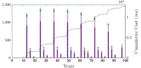
Figure 6 shows the financial costs over time. It can be seen that the cumulative cost difference between Figures 6(a) and 6(b) is almost double across the 100-year timespan being simulated. This is because in Figure 6(b) there is a much greater chance of: 1) incorrect maintenance actions being scheduled which would result in additional costs of materials and financial compensation due to struc-tural possession and 2) the effect of imperfect re-pairs meaning that the condition of the structure does not reset to an A1 condition after every in-tervention, which inevitably reduces the time re-quired before the next intervention is rere-quired.

8 CONCLUSION

MinorA1 MinorB2 MinorB3 MinorB4 MinorB5 MinorB6 MinorC2 MinorC3 MinorC4 MinorC5 MinorC6 MinorD2 MinorD3 MinorD4 MinorD5 MinorD6 MinorE2 MinorE3 MinorE4 MinorE5 MinorE6 MinorF2 MinorF3 MinorF4 MinorF5 MinorF6 MinorG2 MinorG3 MinorG4 MinorG5 MinorG6

0 0.2 0.4 0.6

Probabilit

y

Place

Occupied

(a) Control scenario, without variability.

MinorA1 MinorB2 MinorB3 MinorB4 MinorB5 MinorB6 MinorC2 MinorC3 MinorC4 MinorC5 MinorC6 MinorD2 MinorD3 MinorD4 MinorD5 MinorD6 MinorE2 MinorE3 MinorE4 MinorE5 MinorE6 MinorF2 MinorF3 MinorF4 MinorF5

0 0.2 0.4 0.6

(b) Enhanced scenario, considering variability.

Figure 4: Probability of the element residing in each condition state, aggregated over the entire simulation period.

0 20 40 60 80 100

0 0.2 0.4 0.6 0.8 1

Years

Probabilit

y

(a) Control scenario, without variability.

0 20 40 60 80 100

0 0.2 0.4 0.6 0.8 1

Years

A1 B2 B3 B4 B5 B6 C2 C3 C4 C5 C6 D2 D3 D4 D5 D6 E3 E4 E5 E6 F3 F4 F5 F6

(b) Enhanced scenario, considering variability.

Figure 5: Probability of the element condition over time, aggregated by year.

system. This reduces its usefulness as a decision support tool for bridge portfolio managers.

The purpose of this study was to investigate the sources of variability within bridge asset manage-ment, focusing on human-induced variability, the results of which can help advise where bridge port-folio managers should focus their efforts going for-ward. The following sources of variability were in-vestigated: 1) variability in defect diagnoses caus-ing the wrong type of maintenance to be sched-uled and 2) variability in the intervention process as not all repairs are of equal quality and therefore the associated condition uplift is different. Expert judgement and historical data was used to calcu-late the variability in the processes.

Using an existing WLCC model, two scenar-ios were simulated and their outputs compared. The results show that, when comparing the two scenarios, the enhanced scenario, which consid-ers human-induced variability, predicts greater fi-nancial and operational burden than the control scenario, which does not consider human-induced variability. The enhanced scenario is much more accurate to the real-world system and considers many more of the complexities.

Overall, it is understood that bridge

portfo-lio management is a complex task. The human-induced variability has a significant impact on the management of the bridges as it results in inefficient and ineffective inspection/maintenance teams, which reduces budgetary efficiency too. The results of this study show that even moder-ate amounts of human-induced variability quickly build up in the system to make the whole process much more complex and much more capital inten-sive to manage.

9 ACKNOWLEDGEMENTS

Net-0 10 20 30 40 50 60 70 80 90 1000 0.5 1 ·104

0 10 20 30 40 50 60 70 80 90 100 0

500 1,000 1,500

Years

Yearly

Cost

(

mu

)

Cost of Replacements Cost of Major Repairs Cost of Minor Repairs Cost of Inspections

(a) Control scenario, without variability.

0 10 20 30 40 50 60 70 80 90 100

0 500

1,000

1,500

Years

0 10 20 30 40 50 60 70 80 90 1000

0.5

1

·104

Cum

ulativ

e

Cost

(

mu

)

(b) Enhanced scenario, considering variability.

Figure 6: Cost output of intervention and inspections per year.

work Rail Research Fellow in the Resilience Engi-neering Research Group at the University of Not-tingham. Panayioti Yianni is an Asset Manage-ment Consultant within Jacobs UK’s Asset Man-agement Advisory team. The research was sup-ported by Network Rail and the Engineering and the EPSRC grant reference EP/L50502X/1. They gratefully acknowledge the support of these orga-nizations.

REFERENCES

Andrews, J. (2013). A modelling approach to railway track asset management. Proceedings of the Institution of Me-chanical Engineers, Part F: Journal of Rail and Rapid Transit 227(1), 56–73.

Ben-Akiva, M., F. Humplick, S. Madanat, & R. Ra-maswamy (1993). Infrastructure management under un-certainty: Latent performance approach. Journal of Transportation Engineering 119(1), 43–58.

British Standards Institution (2012). Analysis techniques for dependability — Petri net techniques. Technical re-port.

Frangopol, D. M., M.-J. Kallen, & J. M. van Noortwijk (2004). Probabilistic models for life-cycle performance of deteriorating structures: review and future directions. Progress in Structural Engineering and Materials 6(4), 197–212.

Jensen, K. (1997). A brief introduction to coloured Petri Nets. In E. Brinksma (Ed.), Tools and Algorithms for the Construction and Analysis of Systems, Number 1217 in Lecture Notes in Computer Science, pp. 203–208. Springer Berlin Heidelberg.

Le, B. & J. Andrews (2013). Modelling railway bridge as-set management. Proceedings of the Institution of Me-chanical Engineers, Part F: Journal of Rail and Rapid Transit 227(6), 644–656.

Madanat, S. (1993). Optimal infrastructure management decisions under uncertainty. Transportation Research Part C: Emerging Technologies 1(1), 77–88.

Miyamoto, A., K. Kawamura, & H. Nakamura (2000). Bridge Management System and Maintenance Opti-mization for Existing Bridges. Computer-Aided Civil and Infrastructure Engineering 15(1), 45–55.

Moore, M., B. M. Phares, B. Graybeal, D. Rolander, & G. Washer (2001). Reliability of visual inspection for highway bridges, volume I: Final report. Federal High-way Administration.

Morcous, G. & Z. Lounis (2006). Integration of stochastic

deterioration models with multicriteria decision theory for optimizing maintenance of bridge decks. Canadian Journal of Civil Engineering 33(6), 756–765.

Morcous, G., H. Rivard, & A. Hanna (2002). Modeling bridge deterioration using case-based reasoning. Jour-nal of Infrastructure Systems 8(3), 86–95.

Network Rail (2010a). Handbook for the examination of Structures Part 11A: Reporting and recording examina-tions of Structures in CARRS. NR/L1/CIV/006/11A. Network Rail (2010b). Handbook for the examination of

Structures Part 1C: Risk categories and examination in-tervals. NR/L3/CIV/006/1C.

Network Rail (2010c). Handbook for the examination of Structures Part 2C: Condition marking of Bridges. NR/L3/CIV/006/2C.

Network Rail (2010d). Network Rail Asset Management Policy Justification for Civil Engineering Policy. Network Rail (2012a). Policy on a Page: Structures. Network Rail (2012b). Structures Asset Management Policy

and Strategy. pp. 219.

Neves, L. C. & D. M. Frangopol (2010). Optimization of bridge maintenance actions considering combination of sources of information: Inspections and expert judg-ment. In Bridge Maintenance, Safety, Management and Life-Cycle Optimization: Proceedings of the Fifth In-ternational IABMAS Conference, Philadelphia, USA, 11-15 July 2010, pp. 374. CRC Press.

Petri, C. A. (1962). Communication with Automation. Ph. D. thesis, Mathematical Institute of the University of Bonn, Bonn, Germany.

Phares, B., G. Washer, D. Rolander, B. Graybeal, & M. Moore (2004). Routine Highway Bridge Inspec-tion CondiInspec-tion DocumentaInspec-tion Accuracy and Reliabil-ity. Journal of Bridge Engineering 9(4), 403–413. Technical Strategy Leadership Group (TSLG) (2012). Rail

Technical Strategy. Technical report, Rail Research UK Association.

van Noortwijk, J. M. & H. E. Klatter (2004). The use of lifetime distributions in bridge maintenance and replace-ment modelling. Computers And Structures 82(13–14), 1091–1099.