Vibration frequencies extraction of the Forth Road Bridge using high sampling GPS data

Research Article

Vibration Frequencies Extraction of the Forth Road Bridge

Using High Sampling GPS Data

Jian Wang,

Xiaolin Meng,

Changbiao Qin,

and Jiaohong Yi

1_{School of Environment Science and Spatial Informatics, China University of Mining and Technology, Xuzhou 221116, China} 2_{Sino-UK Geospatial Engineering Centre, The University of Nottingham, Nottingham NG7 2TU, UK}

3_{Nottingham Geospatial Institute, The University of Nottingham, Nottingham NG7 2TU, UK}

Correspondence should be addressed to Jian Wang; [email protected]

Received 3 July 2015; Accepted 8 September 2015

Academic Editor: Salvatore Russo

Copyright © 2016 Jian Wang et al. This is an open access article distributed under the Creative Commons Attribution License, which permits unrestricted use, distribution, and reproduction in any medium, provided the original work is properly cited.

This paper proposes a scheme for vibration frequencies extraction of the Forth Road Bridge in Scotland from high sampling GPS data. The interaction between the dynamic response and the ambient loadings is carefully analysed. A bilinear Chebyshev high-pass filter is designed to isolate the quasistatic movements, the FFT algorithm and peak-picking approach are applied to extract the vibration frequencies, and a GPS data accumulation counter is suggested for real-time monitoring applications. To understand the change in the structural characteristics under different loadings, the deformation results from three different loading conditions are presented, that is, the ambient circulation loading, the strong wind under abrupt wind speed change, and the specific trial with two 40 t lorries passing the bridge. The results show that GPS not only can capture absolute 3D deflections reliably, but also can be used to extract the frequency response accurately. It is evident that the frequencies detected using the filtered deflection time series in different direction show quite different characteristics, and more stable results can be obtained from the height displacement time series. The frequency responses of 0.105 and 0.269 Hz extracted from the lateral displacement time series correlate well with the data using height displacement time series.

1. Introduction

The Global Navigation Satellite Systems (GNSS) positioning technology has been widely used in monitoring dynamic responses of civil structures, such as high-rise building and cable-stayed bridges, for more than twenty years. In order to obtain the deflection and the vibration frequencies of bridges, many efforts have been made by the academic to develop monitoring systems and data processing algorithms.

By using the Global Positioning System (GPS), Leach et al. proposed a monitoring system of a cable-stayed suspension bridge to obtain the deformation and the vibration [1]. In 1995, the capability of GPS for monitoring the structural vibrations was verified with an experiment that was per-formed in the Calgary Tower; a vibration frequency of 0.3 Hz in both north-south and east-west directions was extracted [2]. Two experiments were performed for the extraction of the short-term deformations of the suspension bridge at Tulln in Austria and the results show that the precision of

a GPS monitoring system is about 2 mm for the horizontal coordinates and 4 mm for the height component [3]. To monitor the high frequency characteristic of a bridge, a Leica SR510 receiver of 10 Hz sampling rate and a JNS100 receiver measured at 50 Hz were used and the trials were carried out in a controlled environment; the real bridge monitoring has proved the effectiveness of high sampling GPS [4]. To improve the reliability of a system for bridge deflection monitoring, an integrated GPS/Pseudolites system was proposed and its geometric characteristic was analysed [5]. The vertical natural frequency of the Pierre-Laporte Bridge in Canada was extracted using different algorithms and programs based on GPS monitoring data [6]. A motion simulation table was designed to simulate 2D motion of high-rise building in a horizontal plane and motion of long span bridges in a vertical plane; then a GPS antenna was installed on the table for collecting the data of a simulated motion. It demonstrated that GPS data is accurate enough for monitoring the dynamic response of civil structures [7]. Volume 2016, Article ID 9807861, 18 pages

251.5m

125.8m

A₂

A₁

South North

Ref₁

Ref2

B C D E

F 251.5m

125.8m

BCS of the bridge S

W

N

E

X Y

GPS reference GPS receiver GPS monitoring site F GPS receiver

Figure 1: The devices used to monitor the dynamic responses of the Forth Road Bridge (only the data from site F will be analysed).

0 0.5 1 1.5

L

at. (m)

−0.1 0 0.1

L

o

n

g. (m)

63 64 65 66

H

eig

h

t (m)

5.00 9 Feb 23.00

17.00 11.00 17.00 23.00 5.00 10 Feb 11.00 8 Feb

5.00 9 Feb 5.00 10 Feb 17.00 11.00 17.00 23.00

11.00 8 Feb 23.00

17.00 23.00 5.00 10 Feb 5.00 9 Feb

23.00

17.00 11.00 11.00 8 Feb

Time (hrs/date/month)

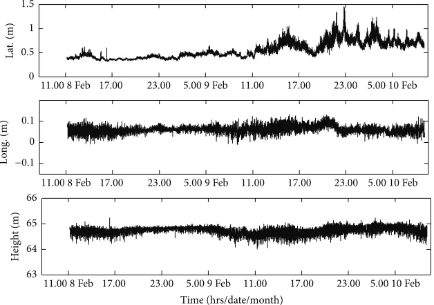
Figure 2: Lateral, longitudinal, and vertical deflection in BCS during the 46 h trial.

A statistical analysis on the outlier level and the accuracy of the real-time kinematic (RTK) and postprocessing kinematic modes were given by Nickitopoulou through using the data collected via a rotating GPS receiver antenna [8]. It can be concluded that GPS is viable to record the responses of forced vibration, decayed free vibration, and ambient vibration of

Temperature Height displacement Mean height displacement

T em p era tu re ( ∘ C) 2 3 4 5 6 7 8 9 10 11 12 23.00 17.00

11.00 8 F

eb

11.00

17.00 23.00

5.00 10 F

eb

5.00 9 F

eb

Cross correlation:−0.55

64 64.2 64.4 64.6 64.8 65 65.2 H eig h t (m)

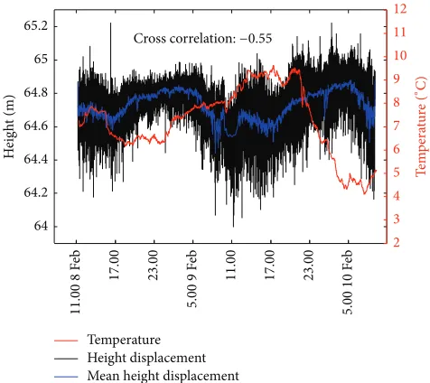
Figure 3: Relation between the air temperature and height deflec-tion at site F.

calculated using the SPACE GASS structural analysis software suite was used to verify the GPS results [10]. The spectral density of deflections monitored via a RTK GPS installed on the Dalian Beida Bridge is in coincidence with that of a finite element model (FEM) [11]. The study also reveals the potential of GPS to measure the deflections and the modal frequencies of rather stiff bridges, far exceeding current limits of the method assumed so far, which was verified via an example by monitoring the oscillations of a 40 m long steel footbridge [12]. GPS was also suitable for the identification of relatively rigid bridges with modal frequencies up to 4 Hz [13]. The mean amplitude of oscillations was calculated with millimetre accuracy via a computer based algorithm using GPS and Robotic Theodolites (RTS) and the method was used to two short span bridges for the structural health monitor-ing [14]. Im et al. reviewed GPS technology for structural health monitoring [15]. GPS is a viable and promising tool for vibration extraction considering the rapid advancement of GPS devices and algorithms. Modal frequencies of the Wilford Bridge are accurately identified using GPS mea-surements with a proposed Multimode Adaptive Filtering (MAF) algorithm and validated by accelerometer data. The fundamental frequency 1.690 Hz of the bridge was detected which is slightly lower than the estimated frequency 1.740 Hz by the structural analysis [16].

Wind loading and multipath effects mainly contribute to low frequency components of bridge dynamics which are difficult to separate and affect early alarming. The amplitude of multipath effect can reach a few centimetres in extreme environment and an adaptive filtering method can mitigate the multipath effect for structural deflection monitoring [17, 18]. Dynamic multipath induced by a passing vehicle for bridges was studied for the first time and certain strategies for modelling were proposed [19]. Actually, monitoring stations have varying circumstance that produces different multipath effects that will be considered in this paper.

This paper proposes an innovative scheme for extracting the vibration frequencies from high sampling GPS data of the Forth Road Bridge. In order to extract the deflection, a Chebyshev high-pass digital filter is designed to eliminate multipath effects and then an FFT is used to extract the frequencies information. The field experiment for the Forth Road Bridge is introduced in detail and the data set of a middle site on the west side of the bridge deck is chosen for analysing the frequency responses. The frequency response in different situations is analysed and compared to obtain the natural frequencies of the bridge.

2. Field Experiment

2.1. The Forth Road Bridge in Scotland. The Forth Road

Bridge, opened to traffic in 1964, links the north of Scotland with Edinburgh and the south, carrying the A90 road of United Kingdom (UK). It has an overall length of 2.5 km and a main span length of 1006 m. The road bridge runs at 3∘ from north. The traffic has increased from 4 million vehicles in 1964 to over 23 million in 2002. In order to investigate the dynamic responses of the Forth Road Bridge, an overall experiment was carried out in 2005 by a research group of the University of Nottingham and the work on the data processing of the deflection and frequency monitoring of the Forth Road Bridge has been reported in 2012 [20].

2.2. Description of the Experiment. During a 46 h observation

period from 8 to 10 February 2005, the data sets were collected by the staff from the former Institute of Engineering Surveying and Space Geodesy (IESSG) at the University of Nottingham; a part of the field data sets is used in this paper to extract the vibration frequencies in various ambient loadings. Five GPS receivers marked as B, C, D, E, and F were fixed to the bridge handrail and two GPS receivers marked as A1 and A2 were located on top of the southern support tower as illustrated in Figure 1 [20].

More details of the receivers’ locations and their spec-ifications are found in [20] and an overall analysis and comparisons of the observations of the GPS receivers were demonstrated in [20]. Data collected at station F is applied to test the proposed scheme as the weather station was installed exactly adjacent to F at the midspan on the western footway. A Leica GX1230 dual-frequency GPS receiver equipped with a Leica AT504 choke-ring antenna was used to collect data at the rate of 10 Hz.

The raw GPS displacement measurements are first trans-formed into the local bridge coordinate system (BCS) using the rotation matrix, the vertical component is represented as the height variations above the mean sea level, and the horizontal displacements are obtained by taking a specific position as the datum.

10−10

10−5

100

M

agni

tude

100 ₁₀1

10−1

10−2

Frequency (rad/s)

−200 −100

0 100 200

Phas

e (deg)

100 101

10−1

10−2

Frequency (rad/s)

−150 −100 −50

0

M

agni

tude (dB)

0 0.5 1 1.5 2 2.5 3 3.5 4 4.5 5

Frequency (Hz)

−400 −300 −200 −100

0

Phas

e (deg)

0 0.5 1 1.5 2 2.5 3 3.5 4 4.5 5

Frequency (Hz)

Figure 4: The corresponding analogue and digit filter.

Yes

No

Low frequency interferences

elimination

GPS sensors GPS data accumulation

High-pass digital filter

FFT transform

Vibration extraction

Counter_{= 0}

counter=counter_{+ 1}

Counter_{≥ T}

Figure 5: Flowchart for vibration frequencies extraction for the Forth Road Bridge.

Lat. displacement Lat. wind speed

Cross correlation:−0.07

−0.03 −0.02

−0.01 0 0.01 0.02 0.03

La

t.

(

m

)

242,500 243,000 243,500 244,000

242,000

GPS time (s)

−5

0 5 10 15 20 25

W

ind sp

eed (km/h)

Figure 6: Lateral displacement and wind speed.

Obvious systematic variations are shown in three direc-tions that are affected by the temperature and wind according to the analysis in literature [20]. It is evident that lateral movements are most significant which reach an order of two meters; this is mainly caused by the ambient wind loadings,

and the largest deflections occur in the second night due to the existence of high wind speeds. The height component of the bridge moves by an order of decimetres, and there exists a close relationship between the height response and ambient temperature variations and traffic loadings; in Figure 3, we can clearly see that a temperature change of about 5.5∘C can be observed during the trial, and it evidently changes the vertical position of the bridge deck, especially the long-term dynamics. As expected, the longitudinal deflections are quite small, and the peak to peak movements are at the order of several centimetres. Three different deformation situations are considered to extract the vibration frequencies of the bridge in this paper, which will be discussed in detail in later sections.

3. Data Processing Scheme

3.1. Description of the Bridge Vibration Signal. The vibration

signal of a bridge monitored by GPS can be expressed by

𝑦 (𝑛) = 𝑀 (𝑛) + 𝐷 (𝑛) + 𝑁 (𝑛) , (1)

−0.015 −0.01

−0.005 0 0.005 0.01 0.015

L

at. disp

lacemen

t (m)

244,000

242,500 243,000 243,500

242,000

GPS time (s)

(a)

×10−3

10−1

10−2 ₁₀0

Frequency (Hz) 0

0.2 0.4 0.6 0.8 1 1.2 1.4 1.6 1.8 2

Am

p

li

tude

(b)

×10−4

0 1 2

Am

p

li

tude

10−1

Frequency (Hz)

(c)

Figure 7: The filtered lateral displacements (a), corresponding vibration frequency ((b), full-scale band), and zoom-in of high frequency component (c).

part;𝐷(𝑛)is the actual dynamic vibrations of the bridge and

𝑁(𝑛) is the noise [16]. To obtain the vibration frequencies of the bridge, low frequency deflections can be isolated using high-pass digital filter that can be designed according to the characteristics of the specific vibration signal, and Chebyshev high-pass digital filter is designed for the vibration frequencies extraction of the Forth Road Bridge in this paper.

3.2. Design of Chebyshev High-Pass Digital Filter. For Type I

Chebyshev filter, the gain response as a function of angular

frequency 𝜔 of 𝑛th-order low-pass filter is equal to the absolute value of the transfer function𝐻_𝑛(𝑗𝜔):

𝐺_{𝑛(𝜔) = 󵄨󵄨󵄨󵄨𝐻𝑛(𝑗𝜔)󵄨󵄨󵄨󵄨 =} 1

√1 + 𝜀2_𝑇2

𝑛(𝜔/𝜔0)

, ₍₂₎

where𝜀is the ripple factor,𝜔₀is the cut-off frequency, and

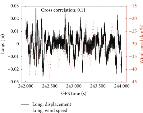
Long. displacement Long. wind speed

Cross correlation: 0.11

242,500 243,000 243,500 244,000

242,000

GPS time (s)

−0.03 −0.02

−0.01 0 0.01 0.02 0.03

L

o

n

g. (m)

−45 −40 −35 −30 −25 −20 −15

W

ind sp

eed (km/h)

Figure 8: Longitudinal displacement and wind speed.

a Chebyshev filter is equal to the number of reactive compo-nents needed to realize the filter using analogue electronics [21].

The ripple is often given in dB. Ripple in dB =

20log₁₀√1 + 𝜀2so that a ripple amplitude of 3 dB results from

𝜀 = 1. The transfer function is then given by

𝐻_𝑎(𝑠) = _2𝑛1_{− 1}∏𝑛

𝑚=1 1

(𝑠 − 𝑠−

𝑝𝑚)

, (3)

where𝑠−_𝑝𝑚are only those poles with a negative sign in front of the real term for the poles.

The bilinear transform is used to convert a transfer function𝐻_𝑎(𝑠)in the continuous-time domain to a transfer function𝐻_𝑑(𝑧)in the discrete-time domain. It maps positions on𝑗𝜔axis, Re[𝑠] = 0, in𝑠-plane to the unit circle,|𝑧| = 1, in𝑧-plane. The bilinear transform essentially uses this first-order approximation and substitutes into the continuous-time transfer function [22],𝐻_𝑎(𝑠):

𝑠 ←󳨀_𝑇2𝑧 − 1_{𝑧 + 1}. (4)

That is,

𝐻_𝑑(𝑧) = 𝐻𝑎(𝑠)󵄨󵄨󵄨󵄨𝑠=(2/𝑇)((𝑧−1)/(𝑧+1))= 𝐻𝑎(_𝑇2𝑧 − 1_{𝑧 + 1}) . (5)

The low-pass Type I Chebyshev filter is transferred from analogue filter to digital filter by using the above bilinear transformation. Subsequently, the low-pass digital Type I Chebyshev filter is transferred into high pass by the following equation [23]:

V−1= −𝑧−1+ 𝛼

1 + 𝛼𝑧−1, (6)

where

𝛼 = cos((𝜔0+ 𝜃0) /2)

cos((𝜔₀− 𝜃₀) /2). (7)

Equation (5) maps 𝑧-plane (low pass) to V-plane (high pass), and𝜔₀and 𝜃₀are cut-off frequencies in𝑧-plane and

V-plane, respectively. The loads of the bridge are varying with different factors, such as wind speeds, traffic flow, and temperature variation; the optimal filter parameters can be determined considering the real deformation. By testing different data sets, the high-pass digital Type I Chebyshev filter with a sampling frequency of 20 Hz is good enough for the data processing of the bridge. In a real application, the filter is sampled into 10 Hz. The critical frequency for pass band is 0.5; pass band attenuation is less than 0.8 dB; the critical frequency for stopband is 0.025 Hz; stopband attenuation is greater than 20 dB. A high-pass digital Type I Chebyshev filter is designed with the above parameters (Figure 4).

3.3. The Scheme for Vibration Frequencies Extraction. The

flowchart for vibration frequencies extraction is summarized in Figure 5. The real-time GPS displacement data sets are input into the designed high-pass digital filter introduced in Section 3.2, to eliminate the low frequency interferences. As a high-pass digital filter cannot be used in a real-time scenario, a GPS data accumulation counter is used to form a time series over a sliding window with a predefined length, to consider the different deformation situations, such as deformation during quiet period or busy period; a varied window length

𝑇can be used, that is, 2000 s or 1000 s, used in this paper. Finally, the vibration frequencies are obtained using the fast Fourier transform (FFT) algorithm.

4. Vibration Frequencies Extraction

4.1. Vibration Frequencies Extraction under Ambient

Circula-tion Loading CondiCircula-tions. In order to evaluate the safety of

the large structures, such as long span bridges and high-rise buildings, it is popular to extract the structural modal parameters such as natural frequencies, mode shapes, and damping ratios from GNSS measurements by using the ambient loadings. The Forth Road Bridge was operated under a heavy traffic flow in the daytime, especially at rush hour; the bridge deck was expected to move under the traffic loads. In this section, we are expected to extract the bridge dynamics under ambient circulation loading conditions; that is, the traffic flow and wind speed are not high.

−0.01 −0.008 −0.006 −0.004

−0.002 0 0.002 0.004 0.006 0.008 0.01

L

o

n

g. dis

p

lacemen

t (m)

242,500 243,000 243,500 244,000

242,000

GPS time (s)

(a)

×10−4

0 1 2 3 4

Am

p

li

tude

100

10−2

Frequency (Hz)

(b)

×10−4

0 1 2 3 4

Am

p

li

tude

10−1

Frequency (Hz)

(c)

Figure 9: The filtered longitudinal displacements (a), corresponding vibration frequency ((b), full-scale band), and zoom-in of high frequency component (c).

firstly; then the output of the high-pass filtered data is used to obtain the vibration frequencies of the bridge. The filtered lateral movements and the corresponding frequencies are demonstrated in Figure 7; it can be seen that the amplitude of the dynamic displacements is small; a low frequency response peaked at 0.067 Hz is significant in the frequency spectra, which is mainly induced by the ambient wind loadings; five higher dominant frequencies with smaller amplitude can also be extracted from the spectra, the extracted frequencies are

listed in Table 1, and this correlates well with our experience for such long span bridge.

−0.08 −0.06 −0.04 −0.02 0 0.02 0.04 0.06 0.08 0.1

H

eig

h

t disp

lacemen

t (m)

242,500 243,000 243,500 244,000

242,000

GPS time (s)

0 0.002 0.004 0.006 0.008 0.01

Am

p

li

tude

10−1

Frequency (Hz)

Figure 10: The filtered height displacements and corresponding frequencies.

Table 1: Vibration frequencies extracted from lateral GPS measurements (𝑋direction of BCS).

Situations Extracted frequencies (Hz) Mean wind speed

(km/h) Common frequencies Distinct frequencies

Ambient circulation loading 0.067 0.073 0.105 0.118 0.269 0.345 0.160 7.30

Strong wind (abrupt wind speed change) 0.069 0.077 0.106 0.110 0.267 0.345 — 52.49 0.068 0.071 0.105 0.110 0.270 0.344 0.097, 0.101 55.83

Two 40 t lorries passing 0.064 0.073 0.103 — 0.268 — 0.132, 0.147 44.75

0 50 100 150

W

ind sp

eed (km/h)

250,000 300,000 350,000

200,000 400,000

GPS time (s)

0 100 200 300 400

W

ind dir

ec

tio

n

(deg)

250,000

200,000 300,000 350,000 400,000

GPS time (s)

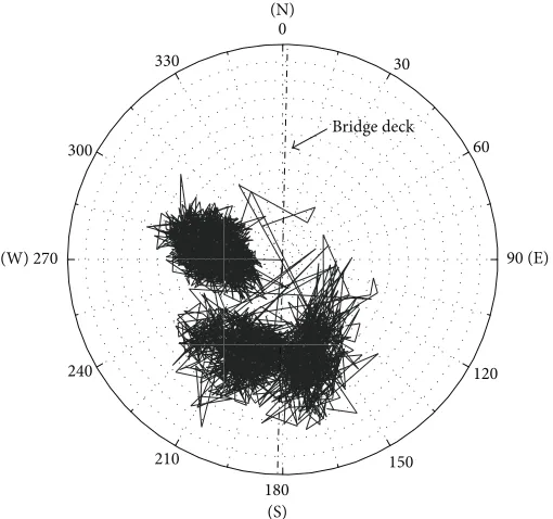
Figure 11: The wind speed and direction during the observation period.

extract from the filtered longitudinal movements; it can be seen that the longitudinal displacements are noisier than lateral displacements; the amplitude of the local frequency peak is not significantly large; thus the frequencies extracted from longitudinal movements are less accurate compared to the results extracted from lateral movements, and higher

frequencies above 0.2 Hz cannot be detected from the filtered longitudinal displacement time series.

The filtered height deflections and the corresponding frequencies are shown in Figure 10, and it can be seen that the frequency response is significant at 0.103 Hz, which is believed to be the natural frequency of the bridge; the amplitude of the frequency response at higher frequency band is obviously smaller than the first natural frequency response. It can be concluded that the vibration frequencies are successfully detected from the high-pass filtered displace-ment time series; that is, the frequencies extracted from the displacement time series in different direction are varied, and this can be explained by the fact that deflections in different direction are actually induced by different loading effects.

4.2. Vibration Frequencies Extraction during Wind Effect.

0

30

60

90 (E)

120

150

180 210

240 300

330

(W) 270

Bridge deck

(S) (N)

Figure 12: The wind direction variation during the observation period.

Wi

n

d

s

p

ee

d

W

in

d

s

p

eed

−100−50

0 50 100

(lo

n

g. km/h)

250,000 300,000 350,000 400,000

200,000

GPS time (s)

250,000 300,000 350,000 400,000

200,000

250,000 300,000 350,000 400,000

200,000

−50 0 50 100

(la

t. km/h)

0 0.5 1 1.5

L

at. deflec

tio

n (m)

Figure 13: The wind speed resolved to BCS and the corresponding deflection.

Due to the stiffness of bridge, the longitudinal movements of the bridge deck are small, while the lateral movements are subject to wind action. The original wind speed data was first resolved to BCS for further analysis. Figure 13 shows wind speed in BCS and the corresponding lateral deflections; it can be seen that the lateral movements have good correlation with high wind speed; the sudden change of wind direction causes the peak vibration of the lateral deflection; once the wind speed keeps stable at a higher speed, the deflection becomes small as the heavy body of the bridge will be dragged down by the force of gravity, and the action of wind speed in lateral and longitudinal direction is cross-conditioning.

Wind speed decreasing Wind speed increasing

Cross correlation: 0.81

−0.5 0 0.5 1

La

t.

(

m

)

−50

0 50 100

W

ind sp

eed (km/h)

330,000

325,000 335,000 340,000

320,000 315,000

GPS time (s)

Lat. wind speed Mean lat. wind speed

Lat. displacement Mean lat. displacement

Figure 14: Lateral displacement and wind speed during the abrupt wind speed changing period.

In our paper, in order to characterize the interaction between the wind speed and deflection, we provide two wind speed changing situations for frequencies extraction using GPS, namely,

(a) wind speed decreasing period: 317001–327000 s; (b) wind speed increasing period: 327001–337000 s.

325,000 325,500 326,000 326,500 327,000 GPS time (s)

−0.03 −0.02

−0.01 0 0.01 0.02 0.03

L

at. disp

lacemen

t (m)

(a)

×10−3

0 0.5 1 1.5 2 2.5 3

Am

p

li

tude

100

10−1

Frequency (Hz)

(b)

×10−4

0 1 2 3 4 5 6 7 8

Am

p

li

tude

10−1

Frequency (Hz)

(c)

Figure 15: The filtered lateral displacements (a), corresponding vibration frequency ((b), full-scale band), and zoom-in of high frequency component (c) during the wind speed decreasing period.

the strong wind causes large movement along lateral direction for the bridge deck.

The lateral deflections contain very slow movements which are beyond the natural frequency band; the bilinear Chebyshev high-pass filter was applied to the original dis-placement time series. The filtered lateral disdis-placements and corresponding vibration frequencies under ambient wind loadings are shown in Figures 15 and 16; the extracted local vibration frequencies less than 5 Hz using GPS displacement

−0.03 −0.02

−0.01 0 0.01 0.02 0.03

L

at. dis

p

lacemen

t (m)

329,000

328,000 328,500

327,500 327,000

GPS time (s)

(a)

×10−3

0 0.5 1 1.5 2 2.5 3

Am

p

li

tude

100

10−1

Frequency (Hz)

(b)

×10−3

0 0.1 0.2 0.3 0.4 0.5 0.6 0.7 0.8 0.9 1

Am

p

li

tude

10−1

Frequency (Hz)

(c)

Figure 16: The filtered lateral displacements (a), corresponding vibration frequency ((b), full-scale band), and zoom-in of high frequency component (c) during the wind speed increasing period.

during the wind speed increasing period is larger than that of the response occurring during the wind speed decreasing period.

The longitudinal displacement measurements during the specific observation period are demonstrated in Figure 17; it can be noted that the wind speed data is noisy, and the correlation between the longitudinal response and the wind data is low. The excitation of longitudinal response is actually a combination of wind loadings, traffic loadings, and

Long. displacement Long. wind speed Cross correlation: 0.14

−0.1

−0.05 0 0.05 0.1

L

o

n

g. (m)

320,000 325,000 330,000 335,000 340,000

315,000

GPS time (s)

−20

0 20 40 60

W

ind sp

eed (km/h)

Figure 17: Longitudinal displacement and wind speed.

325,500

325,000 326,000 326,500 327,000

GPS time (s) −0.01

−0.008 −0.006 −0.004 −0.002 0 0.002 0.004 0.006 0.008 0.01

L

o

n

g. disp

lacemen

t (m)

×10−4

0 1 2 3 4 5

Am

p

li

tude

100

10−1

Frequency (Hz)

Figure 18: The filtered longitudinal displacements and corresponding frequencies during the wind speed decreasing period.

The corresponding filtered height response is shown in Figures 20 and 21; compared to the horizontal response, the amplitude of the height dynamic displacement is obviously larger, which is due to existence of traffic loadings. As can be seen from the frequency spectrum, a significant amplitude peak at 0.102 Hz is detected using the height displacement time series, while a slightly different frequency at 0.104 Hz is observed for the wind speed increasing period; two higher frequency peaks can be detected for both wind loading conditions. The vibration frequencies extracted from height displacement time series seem to be clearer than the frequen-cies extracted using horizontal displacement time series; this demonstrates the superiority of using height deflections for monitoring the frequency response.

4.3. Vibration Frequencies Extraction of the Lorry Loading.

The Forth Road Bridge has experienced increased traffic

loadings since the opening of the bridge, and the heavy traffic loadings play an important role in the bridge deformation, especially for the height deflections. During the second night, a specific trail with two 40 t lorries running on the bridge was carried out to evaluate the pattern of deflection; the bridge was closed off to other traffic during the trial; in addition, the lorries travelled at a low speed manner; the running speed was about 32 km/h. The travelling period used for analysis in this paper was described as follows:

(a) One lorry ran from north to south.

(b) One lorry ran from south to midspan on the west side and stopped and then the other lorry moved north to south.

−0.015 −0.01

−0.005 0 0.005 0.01 0.015

L

o

n

g. dis

p

lacemen

t (m)

327,000 327,500 328,000 328,500 329,000

GPS time (s)

0 1 2 3 4 5

Am

p

li

tude

100

10−1

Frequency (Hz) ×10−4

Figure 19: The filtered longitudinal displacements and corresponding frequencies during the wind speed increasing period.

325,500 326,000 326,500 327,000

325,000

GPS time (s)

−0.1

−0.05 0 0.05 0.1 0.15

H

eig

h

t disp

lacemen

t (m)

0 0.005 0.01 0.015 0.02 0.025 0.03

Am

p

li

tude

100

10−1

Frequency (Hz)

Figure 20: The filtered height displacements and corresponding frequencies during the wind speed decreasing period.

the lorries passing were illustrated in Figure 22; it can be seen that the movements in different direction are deflected by different magnitudes, among which the height component experienced the largest deflections, of the order of ±0.3 m. The bridge experienced downward deflections as the lorry travelled approaching the midspan of bridge, and upward movements were observed when the lorry moved away; this is due to existence of the elastic suspension cable which pulled up the bridge main span. The GPS measured deflections match well with that of FEM predicted results, and occurrence of such bridge deflection can be well explained by the lorries’ mass. It should be noted that the patterns of

the lateral movements do not completely coincide with height movements; actually the lateral movements are partially induced by the ambient wind loadings.

−0.1 −0.05 0 0.05 0.1 0.15

H

eig

h

t disp

lacemen

t (m)

327,000 327,500 328,000 328,500 329,000

GPS time (s)

0 0.005 0.01 0.015 0.02 0.025

Am

p

li

tude

100

10−1

Frequency (Hz)

Figure 21: The filtered height displacements and corresponding frequencies during the wind speed increasing period.

the deformation induced by the low wind loadings, the frequency extraction under high wind loadings becomes clearer.

The filtered longitudinal displacements and extracted frequencies are demonstrated in Figure 24; it can be seen that the amplitude of the dynamic displacements is below 1 cm, and the dynamic response is actually not highly affected by the lorry loading; the frequency characteristic of the response is similar to the response under ambient circulation loading; expect one suspected high frequency at 0.332 Hz detected from the displacement time series; indeed, the high frequency response is vanished due to the existence of high frequency noise.

The corresponding height dynamic displacements and the extracted frequencies are shown in Figure 25; the ampli-tude of the dynamic deflections exceeds 0.1 m; the most significant frequency response is still at 0.103 Hz; it seems that no significant frequency deviation occurs from the frequency spectrum.

4.4. Extracted Frequencies Comparisons. As previously

anal-ysed, we have successfully extracted the vibration frequencies of the bridge under different loading conditions, that is, the ambient circulation loading, strong wind speed sudden changing period, and the specific trial with two 40 t lorries passing the bridge. The results of the extracted frequencies are listed in Tables 1–3. By comparing the results, we can see that the vibration frequencies extracted from the GPS measurements in different direction are varied greatly from each other. Due to the bridge deck stiffness of the bridge deck, the movement along the bridge main axis is small, and low frequency noise can be obviously observed in the longitudi-nal displacement time series, which makes the frequencies extraction more difficult using the peak-picking approach, and the extracted frequencies show different characteristic.

By making a detailed comparison of Tables 1 and 3, we can find that two common frequencies can be extracted from both lateral displacement time series and height displacement time series though the dynamics are induced by different loading effects, that is, 0.105 and 0.269 Hz (slightly different under different ambient loading conditions), so it may be deduced that the two frequencies are the natural frequencies of the bridge. While the other computed frequencies may not indicate the modal characteristics, they mainly indicate excitation frequencies; these frequencies are significant only if they approach modal frequencies with much energy. On the other hand, it should be noted that the extracted frequencies actually varied under different loadings; this will greatly benefit the online damage identification process, because the frequency response is an indicator of structural behaviour. We can also find that height frequency responses are relatively stable for they are mainly affected by the traffic loadings and thermal effects.

5. Conclusions

This paper investigated a GPS deformation trial carried out on the Forth Road Bridge in Scotland. It shows that GPS can capture the absolute 3D deflections of the bridge accurately at a 10 Hz sampling rate. The results have shown that lateral movements highly correlate with the ambient wind loading as the wind speed is high, while the height deflections are mainly caused by the traffic loading and thermal effect; the movement along the bridge main axis is small due to the stiffness of the bridge deck.

349,800 350,000 350,200 350,400 350,600 GPS time (s)

−0.08 −0.06 −0.04

−0.02 0 0.02 0.04 0.06 0.08 0.1

L

at. (m)

(a)

−0.03

−0.02

−0.01

0 0.01 0.02 0.03

L

o

n

g. (m)

349,800 350,000 350,200 350,400 350,600

GPS time (s)

(b)

−0.3

−0.2

−0.1

0 0.1 0.2

H

eig

h

t (m)

349,800 350,000 350,200 350,400 350,600

GPS time (s)

Two40t lorries passing

(c)

Figure 22: Absolute deflections of bridge site F during the two 40 t lorries passing.

Table 2: Vibration frequencies extracted from longitudinal GPS measurements (𝑌direction of BCS).

Situations Extracted frequencies (Hz) Mean wind speed

(km/h) Common frequencies Distinct frequencies

Ambient circulation loading 0.095 0.105 — 0.136 0.149 0.108, 0.117, 0.161 31.96

Strong wind (abrupt wind speed change) 0.091 — 0.129 0.134 0.151 0.184, 0.262 12.21

— — 0.126 0.134 0.151 0.216 16.46

350,600 350,400

350,200 350,000

349,800

GPS time (s) −0.03

−0.02 −0.01 0 0.01 0.02 0.03

L

at. disp

lacemen

t (m)

0 0.5 1 1.5 2 2.5 3 3.5 4

Am

p

li

tude

×10−3

100

10−1

Frequency (Hz)

Figure 23: The filtered lateral displacements and corresponding frequencies.

350,000 350,200 350,400 350,600

349,800

GPS time (s)

×10−4

0 1 2 3 4 5 6 7 8

Am

p

li

tude

100

10−1

Frequency (Hz)

−0.01

−0.005 0 0.005 0.01

L

o

n

g. disp

lacemen

t (m)

Figure 24: The filtered longitudinal displacements and corresponding frequencies.

Table 3: Vibration frequencies extracted from height GPS measurements (𝑈direction of BCS).

Situations Extracted frequencies (Hz) Mean wind speed (km/h)

Ambient circulation loading 0.092 0.103 0.207 0.270 —

Strong wind (abrupt wind speed change) 0.095 0.102 0.205 0.268 —

0.098 0.104 0.204 0.270 —

−0.1 −0.05 0 0.05 0.1 0.15

H

eig

h

t disp

lacemen

t (m)

350,000 350,200 350,400 350,600

349,800

GPS time (s)

0 0.005 0.01 0.015 0.02 0.025 0.03

Am

p

li

tude

10−1 100

Frequency (Hz)

Figure 25: The filtered height displacements and corresponding frequencies.

high-pass filter was presented and applied to the original displacement time series to remove the very slow movements, which do not locate in the structural natural frequency band. The FFT algorithm was applied to the filtered displacement time series, and the vibration frequencies are extracted using the peak-picking approach. The results show that the frequency responses in different directions vary greatly with each other, and the frequency responses at 0.105 and 0.269 Hz extracted from lateral displacement time series correlate well with the data using height displacement time series; the natural frequencies change slightly under different ambient loadings. The approach introduced in this paper can be well applied for the future online bridge monitoring; the structural deterioration and failure will be monitored using the real GPS data in real time, and the frequency response becomes the basis to evaluate the behaviour of the bridge.

Conflict of Interests

The authors declare that there is no conflict of interests regarding the publication of this paper.

Acknowledgments

The data acquisition was sponsored by the Forth Road Bridge. The other colleagues of the University of Nottingham are acknowledged. This work was partially supported by the Fundamental Research Funds for the Central Universities (no. 2014ZDPY15), the Program for New Century Excellent Talents in University (no. NCET-13-1019), a project funded by the Priority Academic Program Development of Jiangsu Higher Education Institutions, and the Cooperative Innova-tion Centre of Jiangsu Province.

References

[1] M. Leach, M. Hyzak, and S. Horoschak, “Validation and analysis of results from a bridge motion monitoring experiment,” in Proceedings of the 49th Annual Meeting of the Institute of Navigation: Future Global Navigation and Guidance, pp. 519– 527, Cambridge, Mass, USA, June 1993.

[2] J. W. Lovse, W. F. Teskey, G. Lachapelle, and M. E. Cannon, “Dynamic deformation monitoring of tall structure using GPS technology,”Journal of Surveying Engineering, vol. 121, no. 1, pp. 35–40, 1995.

[3] A. Wieser and F. Brunner, “Analysis of bridge deformations using continuous GPS measurements,” inProceedings of the 2nd Conference of Engineering Surveying (INGEO ’02), pp. 45–52, Bratislava, Slovakia, November 2002.

[4] G. W. Roberts, E. Cosser, X. Meng, and A. Dodson, “High frequency deflection monitoring of bridges by GPS,”Journal of Global Positioning Systems, vol. 3, no. 1-2, pp. 226–231, 2004. [5] X. Meng, G. W. Roberts, A. H. Dodson, E. Cosser, J. Barnes,

and C. Rizos, “Impact of GPS satellite and pseudolite geometry on structural deformation monitoring: analytical and empirical studies,”Journal of Geodesy, vol. 77, no. 12, pp. 809–822, 2004. [6] A. P. C. Larocca, R. E. Schaal, M. C. Santos, and R. B. Langley,

“Monitoring the deflection of the pierre-laporte suspension bridge with the phase residual method,” inProceedings of the 18th International Technical Meeting of the Satellite Division of the Institute of Navigation (ION GNSS ’05), pp. 2023–2028, Long Beach, Calif, USA, September 2005.

[7] W.-S. Chan, Y.-L. Xu, X.-L. Ding, Y.-L. Xiong, and W.-J. Dai, “Assessment of dynamic measurement accuracy of GPS in three directions,”Journal of Surveying Engineering, vol. 132, no. 3, pp. 108–117, 2006.

[9] X. Meng, A. H. Dodson, and G. W. Roberts, “Detecting bridge dynamics with GPS and triaxial accelerometers,”Engineering Structures, vol. 29, no. 11, pp. 3178–3184, 2007.

[10] C. Watson, T. Watson, and R. Coleman, “Structural monitoring of cable-stayed bridge: analysis of GPS versus modeled deflec-tions,”Journal of Surveying Engineering, vol. 133, no. 1, pp. 23–28, 2007.

[11] T. H. Yi, H. N. Li, and M. Gu, “Full-scale measurements of dynamic response of suspension bridge subjected to environmental loads using GPS technology,” Science China-Technological Sciences, vol. 53, no. 2, pp. 469–479, 2010. [12] F. Moschas and S. Stiros, “Measurement of the dynamic

displacements and of the modal frequencies of a short-span pedestrian bridge using GPS and an accelerometer,”Engineering Structures, vol. 33, no. 1, pp. 10–17, 2011.

[13] P. Psimoulis, S. Pytharouli, D. Karambalis, and S. Stiros, “Poten-tial of Global Positioning System (GPS) to measure frequencies of oscillations of engineering structures,”Journal of Sound and Vibration, vol. 318, no. 3, pp. 606–623, 2008.

[14] P. A. Psimoulis and S. C. Stiros, “A supervised learning computer-based algorithm to derive the amplitude of oscilla-tions of structures using noisy GPS and Robotic Theodolites (RTS) records,”Computers & Structures, vol. 92-93, pp. 337–348, 2012.

[15] S. B. Im, S. Hurlebaus, and Y. J. Kang, “Summary review of GPS technology for structural health monitoring,”Journal of Structural Engineering, vol. 139, no. 10, pp. 1653–1664, 2013. [16] J. Y. Yu, X. L. Meng, X. D. Shao, B. F. Yan, and L. Yang,

“Iden-tification of dynamic displacements and modal frequencies of a medium-span suspension bridge using multimode GNSS processing,”Engineering Structures, vol. 81, pp. 432–443, 2014. [17] A. Dodson, X. Meng, and G. Roberts, “Adaptive method for

multipath mitigation and its applications for structural deflec-tion monitoring,” inProceedings of the International Symposium on Kinematic Systems in Geodesy, Geomatics and Navigation (KIS ’01), pp. 5–8, Banff, Canada, June 2001.

[18] G. W. Roberts, X. Meng, and A. H. Dodson, “Using adaptive fil-tering to detect multipath and cycle slips in GPS/accelerometer bridge deflection monitoring data,” inProceedings of the 22nd International Congress of the FIG, pp. 19–26, Washington, DC, USA, April 2002.

[19] F. Moschas and S. Stiros, “Dynamic multipath in structural bridge monitoring: an experimental approach,”GPS Solutions, vol. 18, no. 2, pp. 209–218, 2014.

[20] G. W. Roberts, C. J. Brown, X. Meng, O. Ogundipe, C. Atkins, and B. Colford, “Deflection and frequency monitoring of the Forth Road Bridge, Scotland, by GPS,”Bridge Engineering, vol. 165, no. 2, pp. 105–123, 2012.

[21] B. A. Shenoi,Introduction to Digital Signal Processing and Filter Design, John Wiley & Sons, 2005.

[22] J. H. Lodge and M. M. Fahmy, “The bilinear transformation of two-dimensional state-space systems,”IEEE Transactions on Acoustics, Speech, and Signal Processing, vol. 30, no. 3, pp. 500– 502, 1982.

International Journal of

Aerospace

Engineering

http://www.hindawi.com Volume 2014

Robotics

Hindawi Publishing Corporation

http://www.hindawi.com Volume 2014

Hindawi Publishing Corporation

http://www.hindawi.com Volume 2014

Active and Passive Electronic Components

Control Science and Engineering

Journal of

Hindawi Publishing Corporation

http://www.hindawi.com Volume 2014 Machinery

Hindawi Publishing Corporation

http://www.hindawi.com Volume 2014

Hindawi Publishing Corporation http://www.hindawi.com

Journal of

Engineering

Submit your manuscripts at

http://www.hindawi.com

VLSI Design

Hindawi Publishing Corporation

http://www.hindawi.com Volume 2014

Hindawi Publishing Corporation

http://www.hindawi.com Volume 2014

Shock and Vibration

Hindawi Publishing Corporation

http://www.hindawi.com Volume 2014

Civil Engineering

Acoustics and VibrationAdvances in

Hindawi Publishing Corporation

http://www.hindawi.com Volume 2014

Hindawi Publishing Corporation

http://www.hindawi.com Volume 2014

Electrical and Computer Engineering

Journal of

Advances in OptoElectronics

Hindawi Publishing Corporation

http://www.hindawi.com Volume 2014

The Scientific

World Journal

Hindawi Publishing Corporation

http://www.hindawi.com Volume 2014

Sensors

http://www.hindawi.com Volume 2014

Modelling & Simulation in Engineering

Hindawi Publishing Corporation

http://www.hindawi.com Volume 2014

Hindawi Publishing Corporation

http://www.hindawi.com Volume 2014 Chemical Engineering

International Journal of Antennas and

Propagation International Journal of

Hindawi Publishing Corporation

http://www.hindawi.com Volume 2014

Hindawi Publishing Corporation

http://www.hindawi.com Volume 2014

Navigation and Observation International Journal of

Hindawi Publishing Corporation

http://www.hindawi.com Volume 2014

Distributed

Sensor Networks