Computational studies on pressure distribution around a bending 5:1 rectangular cylinder

8th International Colloquium on Bluff Body Aerodynamics and Applications Northeastern University, Boston, Massachusetts, USA June 7 - 11, 2016

BBAA VIII

Computational studies of pressure distribution around

a bending 5:1 rectangular cylinder

Dinh Tung Nguyen

, David Hargreaves

, John Owen

a

University of Nottingham, Nottingham, United Kingdom, [email protected]

b

University of Nottingham, Nottingham, United Kingdom, [email protected]

c

University of Nottingham, Nottingham, United Kingdom, [email protected]

SUMMARY:

This paper describes the development and testing of a numerical model, based around the Large Eddy Simulation model, of a flexible 5:1 rectangular cylinder. We report on the vortex-induced vibration (VIV) of the bending cylinder, which is an analogue for a flexible bridge deck. Compared with a 3D heaving sectional model, distinct differences in surface pressure distributions and Strouhal number in the span-wise direction were found. In addition, certain span-wise flow features were thought to trigger the lock-in when the flexible model underwent the bending VIV response.

Keywords: Bridge aeroelasticity, 5:1 ratio, Rectangular cylinder, Pressure distribution, CFD, Fluid-structure interation.

1. INTRODUCTION

The rectangular cylinder has been considered as a simplified geometry of many structures in the built environment including the main section of a suspension bridge. It differs from the circular cylinder in that the rectangular cylinder is characterised by the permanent separation at the leading edges causing two unstable shear layers along surfaces of the body. The aspect ratio (i.e. the ratio between the width and the depth of the cross section) and the Reynolds numbers have been found to control their properties together with the vortex structure in the wake region (Okajima, 1982; Ozono et al., 1992; Schewe, 2013). More importantly, the interaction between the leading-edge shear layer and the von Karman vortex shed from the trailing edge governs the dynamic responses (Kotmasu and Kobayashi, 1980; Matsomoto et al., 2008).

The aerodynamics of the flow around and the aeroelasticity of the rectangular cylinder have also been investigated by the use of numerical methods. Due to the complexity of the problem and the limitation of computational power, the simulation was initially restricted to model the flow field around 2D static cylinder only with the use of the two-equation Unsteady Reynolds-Averaged Navier-Stokes (URANS) models. Later, 3D simulations using the LES model have become more available focusing on uncovering the characteristics of the separation bubbles, the effect of the afterbody length on the separation and reattachment of the flow and the coherence structure of the surface pressure around a static rectangular cylinder (Bruno et al., 2010). The LES approach was also coupled with a structural solver to model the fluid-structure interaction (FSI) of a 3D elastically supported rectangular cylinder at a low Reynolds number flow (Sun et al., 2008). The work highlighted the suitability of the LES model to capture the inherent unsteadiness in FSI problems and to maintain the turbulence structure in the wake region in contrast to over-dissipation of the URANS turbulence models. Daniels et al. (2004) also applied this method to predict the effect of the free-stream turbulence on the aerodynamic behavior of a static and elastically mounted 4:1 rectangular cylinder. The use of the LES approach is still limited due to its computationally expensive near-wall treatment. In addition, Bruno et al., (2011) showed results of 3D LES simulations in the application of the bridge aeroelasticity were very susceptible to the level of discretisation in the span-wise direction.

In this project, utilising the High Performance Computer at the University of Nottingham, the aforementioned coupling approach between the LES model and the FSI solver is applied to model the flow field and simulate the aeroelasticity of a static and elastically mounted 3D sectional rectangular cylinder of the 5:1 aspect ratio in the smooth flow. In addition, a 3D flexible model is built and a mode shape is integrated in the FSI solver to simulate its responses as a half of the bridge deck. The surface pressure distribution and the VIV responses of the flexible model in the bending mode will be compared against those of the sectional model in the heaving mode to uncover the important flow features in the span-wise direction.

2. APPLICATION

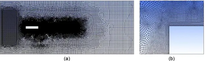
The computational studies were calculated using the open-source CFD software OpenFOAM v2.2.2. The unsteady flow around the rectangular section was modelled using a LES model. The Smagorinsky model was applied to model sub-grid scale stresses. The computational domain and the key boundary conditions are summarised in Figure 1a. A zero gradient condition for velocity and constant value of zero pressure were imposed on the oulet. As for the inlet, a non-zero x-component wind speed and a zero gradient condition for pressure were specified simulate the smooth flow. The movingWallVelocity was applied on the surface of the model to accurately model a zero normal-to-wall velocity component particularly in the dynamic simulation. The computational domain was hybrid in the x-z plane (Figure 2a) and structured in the y direction. An inflation layer, which was a six-cell-thick structure grid, was imposed around the model. The discretisation next to the model was x/B = 2z/B = 410-3 (Figure 2b). Different values of the span-wise discretisation, y, span-wise length, L, and boundary conditions of the y

2.1. Static Simulation

The OpenFOAM solver pimpleFoam was used to simulation the flow around the 3D static sectional model at 3 different wind speeds, 1, 2 and 4 ms-1. At each wind speed, the surface pressure data was extracted at selected points to evaluate the pressure correlation and pressure distribution.

2.2. Dynamic Simulation

As for the 3D sectional model, the coupling scheme procedure between the OpenFOAM solver pimpleDyMFoam and the mass-damper-spring equation was utilised. The mode shape equation is set as 1(y) = 1, i.e. the 3D section model behaved like a rigid body having a mass per unit length of 𝑚̅ = 4.7 kg/m. The Scruton number was Scr = 9.64. The model was restrained to

respond in the heaving mode only with the natural frequency of fn,h = 1.2 Hz. The wind speed was increased from 0.1 ms-1 to 2.5 ms-1 in increments of 0.1 ms-1 during the lock-in.

For the 3D flexible model, the mode shape 1(y) = osin[/(2Lo)y] with the scaling factor o = 0.363 was used so that the model was treated as a cantilever which could exhibit half of the

first bending mode (Figure 3). The selection of this scaling factor allowed a unit generalised mass. All of the structural parameters were similar to the 3D sectional model. It is noted the inclusion of the L1 and Labutment in Figure 3 was to reduce the effect of the symmetryPlane boundary condition on the flow field around the half-span Lo section.

As for the dynamic simulation, a dynamic mesh algorithm was prescribed and implemented to accommodate the deformation of the model. As shown in Figure 1b, the computational domain is divided into 9 different blocks. Blocks 1 and 3 are rigid where cells are fixed relatively to the model. The other blocks are grouped into the buffer zone where cells are deformed and displaced to facilitate the displacement of the model. In addition, the conventional serial staggered algorithm is applied to model the coupling between the fluid, structure and dynamic mesh.

(a) (b)

Figure 1. Computational domain and boundary conditions (a) and illustration of 9 different blocks in the computational domain (b).

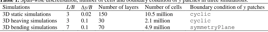
Table 1. Span-wise discretisation, number of cells and boundary condition of y patches in three simulations. Simulations L/B y/B Number of layers Number of cells Boundary condition of y patches

3D static simulations 3 0.02 150 10.5 million cyclic

3D heaving simulations 3 0.1 30 2.1 million cyclic

Figure 2. Computational grid in the x-z plane for the entire domain (a) and aroud the leading edge (b).

Figure 3. Schematic diagram of the simulated flexible model. Lo = 5B is the half of the span.

3. RESULTS AND DISCUSSION

3.1. Static Simulation

Table 1 summaries force coefficients and Strouhal number at three different Reynolds numbers in a comparison against the on-going wind tunnel study (Nguyen et al., 2016) and another wind tunnel study (Schewe, 2013). The width, B, was used as the characteristic length scale for all coefficients. Except for the values of CL, there was a good agreement between the current computational study and other wind tunnel tests. This study predicted a negative value of CL, which was also reported in other LES simulations (Bruno et al., 2010). One possible reason for this discrepancy was the slight asymmetry between the top and bottom halves of the unstructured grid which may lead to the flow being resolved differently on either side of the model.

Table 2. Force coefficients and Strouhal number obtained from computational and wind tunnel studies.

Re St 𝐶𝐷 𝐶𝐿 𝐶𝐿′

Current CFD studies

6700 0.608 1.205 -0.056 0.081

13000 0.600 1.030 -0.059 0.075

27000 0.609 1.030 -0.063 0.059

WT studies - Schewe (2013) 6000 – 40000 0.555 1.210 0 0.08 WT studies - Nguyen et al. (2016) 50000 0.640 1.191 0.034 -

Figure 4. Pressure correlation in the span-wise direction. Wind tunnel results from Ricciardelli and Marra (2008) at the Reynolds number of Re = 63600.

Figure 5. Span-wise coherence of pressure. The top row is close to the leading edge while the other is close to the trailing edge.

3.2. Heaving Simulation

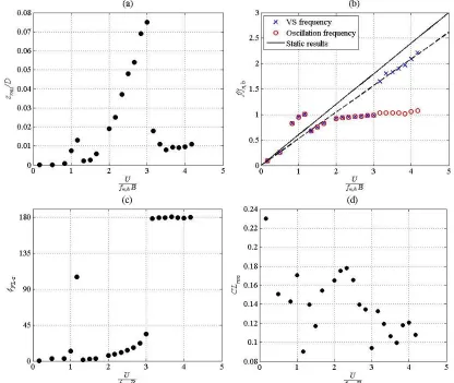
Figure 6c showed the variation of the phase of the lift force against the displacement with the wind speed. As the amplitude of the response increased, the in-phase component of the lift force became less and when the cylinder moved out of the lock-in region, the lift force suddenly became out-of phase. This transition indicated there was a dramatic change in the flow structure around the cylinder which was responsible for the lock-out.

Figure 6. Heaving VIV response of the sectional model in the smooth flow.

Figure 7. Variation of the span-wise pressure correlation around the leading and trailing edges as the cylinder experienced the lock-in.

3.3. Bending Simulation

As can be seen in Figure 8, the VIV response at the mid-span (y/B = 5) of the flexible model shared some common characteristics as the sectional model regarding the onset reduced wind speeds of two VIV lock-in regions, the lock-in of the vortex-shedding frequency and the reduced wind speed where the maximum response occurred.

At the reduced wind speed of Ur = 3 which was at the peak of the larger VIV response, the pressure distribution measured at different span-wise positions is shown in Figure 9; s is measured from the stagnation point on the front face. In contrast to the heaving model where flow features on the side surfaces were uniform in the span-wise direction, the geometry of the separation bubble varied significantly from the fixed end (y/B = 0) to the end having the maximum displacement (y/B = 5). Also the frequency of the lift force shifted from the value defined by the Strouhal number (Peak A in Figure 10a and b) to the natural frequency (Peak B in Figure 10b and c).

Figure 9. Pressure distribution on the top and bottom surfaces at three different span-wise positions.

Figure 10. Spectra of the lift forces measured at different span-wise positions.

Figure 11. Spectra of the z-component velocity measured at a distance B behind the model and D/2 from the top surface.

The velocity measured behind the model also showed a variation in flow features in the span-wise direction (Figure 11). At the fixed end, the dominant flow feature was the von Karman vortex shed from body at the frequency defined by the Strouhal number (Peak A in Figure 11a). Towards the end having the maximum displacement, the motion-induced vortex became dominant (Peak B in Figure 11b); the flow feature found at the static end was still present but their relative strength varied along the span-wise length.

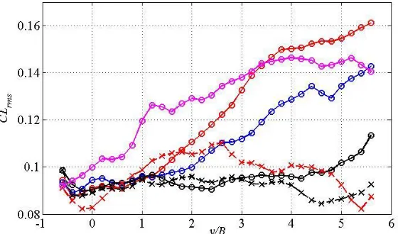
the VIV lock-in. Around the moving end (y/B = 5), the general behaviour was very similar to what observed on the sectional model, which was a sudden change in the phase angle at Ur = 3.33 indicating the lock-out and the fluctuating lift force was maximum at Ur = 2.33. However, in the span-wise direction, some distinct flow feature was observed. At the onset of the lock-in which was around Ur = 2, regarding the phase relationship, the lift force was behind the displacement at the moving end (y/B = 5). Also, the span-wise profile of 𝐶_𝐿′ at this reduced wind speed showed less difference for the portion of y/B > 1. When the amplitude increased, this difference was magnified; more fluctuation in the lift force was observed around the moving end. The phase profile showed the lift force was in-front of the displacement and the in-phase component of the lift force reached the peak at Ur = 2.33 and gradually decreased. Eventually, a sudden change in the gradient of the span-wise profile of the phase lag indicated the lock-out.

These results showed that the on-set of the lock-in potentially did not relate to the aerodynamics of the flow field around the moving end where the maximum displacement is expected. Instead, some flow feature occurred around the portion between y/B = 1 and 3 could be the triggering mechanism for the lock-in. As the amplitude of the response increased, the flow feature was either diffused by the pressure gradient occurring in the span-wise direction or shifted towards the moving end and accounted to building up the amplitude of the VIV response.

Figure 12. Span-wise varitaion of the phase angle of the lift force against the displacement as the model experienced the lock-in.

4. CONCLUSIONS

Together with the on-going wind tunnel study, the heaving simulation in this computational study has shown the VIV of the 5:1 rectangular cylinder occurred due to two separate mechanism. The motion-induced leading edge vortex was responsible as a triggering mechanism of the lock-in; the flow feature around the trailing edge where the leading edge vortex impinged on the surface induced a raise in the local suction leading to an increase in the response.

The bending simulation using the flexible model has showed similar behaviour regarding the VIV. The analysis of the surface pressure distribution and the velocity in the wake region has revealed distinct aerodynamics of the flow field in a comparison against the heaving model including a span-wise variation in the pressure distribution and wake structure. Further analysis also showed that, in this case, the VIV lock-in of the flexible model could be originated by some flow features around the portion between y/B = 1 and 3, not exactly at the moving end where the maximum displacement was expected to be observed. As the amplitude was built-up, increased pressure gradient in the span-wise direction could potentially diffuse or shift this flow feature towards to the moving end leading to an increase in the response.

REFERENCES

Bruno, L., Coste, N. and Fracos, D., 2011. Simulated flow around a rectangular 5:1 cylinder: Spanwise dicretisation effects and emerging flow features. Journal of Wind Engineering and Industrial Aerodynamics, 104 – 106(0), 203 – 215.

Bruno, L., Grancos, D., Coste, N. and Bosco, A., 2010. 3D flow around a rectangular cylinder: A computational study. Journal of Wind Engineering and Industrial Aerodynamics, 98(6-7), 263 – 276.

Daniels, S., Castro, I. and Xie, Z.T., 2004. Free-stream turbulence effects on bridge decks undergoing vortex-induced vibrations using large-eddy simulation. In the Proceeding of 11th UK Conference on Wind Engineering, Birmingham, UK.

Kiya, M. and Sasaki, K., 1985. Strucutre of large-scale vortices and unsteady reverse flow in the reattaching zone of turbulent separation bubble. Journal of Fluid Mechanics, 154, 463 – 491.

Komatsu, S. and Kobayashi, H., 1980. Vortex-induced oscillation of bluff bodies. Journal of Wind Engineeering and Industrial Aerodynamics, 6(3/4), 335 – 360.

Matsumoto, M., Yagi, T., Tamaki, H. and Tsubota, T., 2008. Vortex-induced vibration and its effect on torsional flutter in the case of B/D = 4 rectangular cylinder. Journal of Wind Engineering and Industrial Aerodynamics, 96(6 – 7), 971 – 983.

Nakamura, Y., Ohya, Y. and Tsuruta, H, 1991. Experiments on vortex shedding from flat plates with square leading and trailing edge. Journal of Fluid Mechanics, 222, 437 – 447.

Nguyen, D.T., Owen, J.S. and Hargreaves, D.M., 2016. Wind tunnel studies of pressure distribution around a 5:1 rectangular cylinder. BBAA VIII International Colloquium on Bluff Bodies Aerodyanmics & Applications, Boston, USA.

Okajima, A., 1982. Strouhal number of rectangular cylinders. Journal of Fluid Mechanics, 123, 379 – 398.

Ozono, S., Ohya, Y., Nakamura, Y. and Nakayama, R., 1992. Stepwise increase in the Strouhal number for flows around flat plates. International Journal for Numerical Methods in Fluid, 15(9), 1025 – 1036.

Ricciardelli, F. and Marra, A.M., 2008. Sectional aerodynamic forces and their longitudinal correlation on a vibrating 5:1 rectangular cylinder. BBAA VI International Colloquium on Bluff Bodies Aerodynamics & Applications, Milano, Italy.

Scanlan, R.H., 1997. Amplitude and turbulence effects on bridge flutter derivatives. Journal of Structural Engineering, 123(2), 232 – 236.

Schewe, G., 2013. Reynods-number-effect in flow around a rectangular cylinder with aspect ratio 1:5. Journal of Fluids and Structures, 36(0), 15 – 26.