Measuring Exchange Rate Flexibility by
Regression Methods
Michael Bleaney* and Mo Tian**
*School of Economics, University of Nottingham, U.K.
**School of Management, Swansea University, U.K.
Abstract
A new and easily implemented regression method is proposed for generating an index of exchange rate flexibility, whilst simultaneously identifying anchors of pegged currencies. The method can distinguish floats from pegs, including those with occasional devaluations. An annual index is calculated that can be compared with other regime classification schemes, or used directly in empirical research as a measure of exchange rate flexibility. Different categories in the IMF’s de facto classification, and also in the Reinhart-Rogoff classification, are associated with significantly different average values of the index. Further analysis of managed floats shows that they have a strong tendency to track the US dollar.
Keywords:
exchange rates, currency pegs, tradeJEL No.:
F311
Introduction
Until 1998 the International Monetary Fund reported only a country’s self-declared exchange
rate regime, chosen from amongst a defined set of categories such as various types of peg,
managed floating or independently floating (see Habermeier et al., 2009, Appendix B, for a
brief history of the IMF classification system). Dissatisfaction with the resulting outcomes,
eloquently expressed by Calvo and Reinhart (2002), led to the development of alternative
methods based on factual data such as exchange rate movements, reserve volatility and
interest rate differentials (Levy-Yeyati and Sturzenegger, 2005; Reinhart and Rogoff, 2004;
Shambaugh, 2004). The IMF also began to record its own de facto assessment of the regime,
alongside the reported de jure classification, using the same taxonomy. The weakness of this
effort is that it conspicuously failed to develop a new consensus in classifying exchange rate
regimes, since the new systems showed a low correlation with one another (Bleaney and
Francisco, 2007; Frankel and Wei, 2008). An extended discussion of these classification
systems appears in Klein and Shambaugh (2010, Ch. 3), and also in the review article by
Rose (2011). Bleaney et al. (2015) argue that different criteria for drawing regime
boundaries, rather than differences in statistical approaches, are the primary reason for the
disappointingly high level of disagreements between classification schemes.
The schemes that seek to produce an alternative to the IMF classification by calendar
year use different statistical criteria. Levy-Yeyati and Sturzenegger (2005) use cluster
analysis based on movements in exchange rates, international reserves and interest rates.
Reinhart and Rogoff (2004) prefer to use parallel-market exchange rates (if they exist), and
discount large movements in up to 20% of observations, in an attempt to distinguish one-time
devaluations from floats. Shambaugh (2004) defines a peg by small monthly exchange rate
None of these approaches uses regression methods. Regression methods have been
successfully used to identify the basket of anchor currencies to which a currency is pegged
(Frankel and Wei, 1995). More recently, Bénassy-Quéré et al. (2006) and Frankel and Wei
(2008) have independently suggested that similar regression methods can distinguish pegs
from floats as well. In this paper, we pursue a similar line of inquiry that, in our view,
improves on previous work. We show that regression analysis can be used to generate
statistics that distinguish floats from pegs, including those with occasional devaluations, with
a high degree of accuracy. It is also a simple way of generating annual measures of exchange
rate flexibility, requiring only end-of-month exchange rate data.
The rest of the paper is organised as follows. In Section Two, previous approaches to
exchange rate regime classification by regression methods are reviewed. Our alternative is
presented in Section Three. Section Four shows the results of our method by IMF de facto
regime category, applied to two separate periods: 1999-2005 and 2006-13. Some illustrative
examples are given in Section Five. In Section Six robustness to the choice of numeraire
currency is discussed. Section Seven examines managed floats more deeply. Section Eight
investigates whether the system can be used to generate annual measures of exchange rate
flexibility. Conclusions are presented in Section Nine.
2
Literature Review
Exchange rate classification schemes are based on the idea that, at least at either end of the
spectrum, exchange rates behave quite differently, even if there are some intermediate cases
that are difficult to classify. Consider a target zone with a central rate of x and permitted
deviation of z, so the zone is (x ± z). If z is small, the exchange rate will have relatively low
small, and so these regimes can be identified as pegs. Finding an appropriate boundary
between pegs and floats is problematic, however, particularly in cases where x undergoes a
step change (a realignment) or follows a trend (a crawling peg or band), or where no value of
x or z is announced but the data suggest that the unannounced policy regime is effectively
some kind of target zone (a managed float). We now briefly review previous attempts to use
regression methods to distinguish pegs from floats.
The standard regression specification for identifying the basket of currencies to which
currency i is pegged (e.g. Frankel and Wei, 1995) relates exchange rate movements of
currency i against some numeraire currency N to movements of potential anchor currencies
against N:
∆ln 𝐸(𝑖, 𝑁)𝑡 = 𝑎 + 𝑏∆ ln 𝐸(𝑈𝑆𝐷, 𝑁)𝑡+ 𝑐∆𝑙𝑛𝐸(𝐸𝑈𝑅, 𝑁)𝑡+ 𝑑∆𝑙𝑛𝐸(𝑌𝐸𝑁, 𝑁)𝑡+ 𝑢𝑡 (1)
where USD is the US dollar, EUR is the euro, YEN is the Japanese yen, E(i, N) is the number
of units of currency i per unit of currency N, and ∆ is the first-difference operator. If
currency i is pegged to a single one of these currencies, the coefficient of that currency
should be one, and of the others zero; if the basket is correctly identified, the three
coefficients should sum to one.
The issue is whether a similar equation can also distinguish floats from pegs, as has
been claimed by Bénassy-Quéré et al. (2006) and Frankel and Wei (2008). Bénassy-Quéré et
al. (2006) avoid the choice of a numeraire currency by noting that, if b+c+d = 1, then a
weighted average of exchange rates of currency i against the three anchors should remain
unchanged:
After estimating equation (2), the authors focus on the estimates of the individual coefficients
b, c and d. They identify a currency as floating only if none of them is significantly different
from zero. This approach appears to suffer from two drawbacks. One is that, because of the
focus on statistical significance, the standard errors of the coefficients could have as much
influence on the result as the point estimates. The other is that, given the constraint that the
estimated coefficients must sum to one, the test is biased towards rejecting the null; and
indeed less than 10% of the sample is identified as floats (Bénassy-Quéré et al., 2006, Table
3). As we shall see later, even freely floating currencies tend to co-move with others with
which they have strong trading links, and are therefore likely in many cases to have non-zero
euro or US dollar coefficients.
Frankel and Wei (2008) augment equation (1) with an exchange market pressure
variable (EMP), which is equal to the log changes in the exchange rate of currency i against N
minus changes in the logarithm of the ratio of international reserves to the monetary base.
They thus estimate:
∆ln 𝐸(𝑖, 𝑁)𝑡 = 𝑎 + 𝑏∆ ln 𝐸(𝑈𝑆𝐷, 𝑁)𝑡+ 𝑐∆𝑙𝑛𝐸(𝐸𝑈𝑅, 𝑁)𝑡+ 𝑑∆𝑙𝑛𝐸(𝑌𝐸𝑁, 𝑁)𝑡+ 𝑓𝐸𝑀𝑃𝑡
+𝑢𝑡 (3)
In fact Frankel and Wei arrive at this specification by including the British pound as an
additional anchor, and then subtracting the pound-numeraire exchange rate from all the other
exchange rate variables to impose the condition that the basket weights sum to one, without
weights using the pound as numeraire.1 They focus on the coefficient of this EMP variable,
arguing that it will be close to zero for pegs, and significantly different from zero for floats.
They broadly confirm this pattern using twenty example currencies. Slavov (2013) applies
this method to investigate the behaviour of nominally floating currencies in sub-Saharan
Africa.
Apart from the fact that the test is not infallible (Australia is an example, as Frankel
and Wei point out), there are some econometric problems here. One component of the EMP
variable is the dependent variable itself, so that component should always have a coefficient
of one, as well as being necessarily correlated with the error term, which introduces bias into
the estimates. The reserves component is also endogenous to exchange rate changes because
the money supply is denominated in domestic currency and reserves in foreign currency.
When the exchange rate depreciates, the ratio of reserves to the monetary base will tend to
increase even if reserves remain unchanged.
3
A New Approach
In this paper we start from the position that, for identifying the type of regime (as opposed to
the possible basket of anchor currencies), the appropriate statistics from a regression equation
like (1) should be based on the volatility and pattern of residuals rather than the estimated
coefficients. At a second stage, if the relevant statistics indicate a peg by whatever criterion is
chosen, then the coefficients can be used to identify the anchor basket.
Our baseline regression is:
∆ln 𝐸(𝑖, 𝑁)𝑡 = 𝑎 + 𝑏∆ ln 𝐸(𝑈𝑆𝐷, 𝑁)𝑡+ 𝑐∆𝑙𝑛𝐸(𝐸𝑈𝑅, 𝑁)𝑡+ 𝑢𝑡 (4)
1 This arises because, for any currency j, ln E(j, N) – ln E(GBP, N) = ln E(j, GBP). The original numeraire
simply disappears from the estimated equation, which reduces to an unrestricted regression with the GBP as
The numeraire currency is the Swiss franc. Initially we included the Japanese yen as well, as
in equation (1), but its coefficients were almost always insignificant. Instead we use the yen
as an alternative numeraire, to check the sensitivity of the results to the choice of numeraire.
For some currencies we added other potential anchor currencies to the equation, as follows:
South African Rand – added for Botswana, Lesotho, Namibia and Swaziland.
Indian Rupee – added for Bangladesh, Bhutan, Maldives, Nepal, Pakistan, Seychelles and Sri
Lanka.
Australian and New Zealand Dollars – added for Fiji, Kiribati, Samoa, Solomon Islands,
Tonga and Vanuatu.
Singapore Dollar – added for Brunei.
To measure volatility, we use the root mean square error (RMSE) and the R-squared
of equation (4).2 We expect the RMSE to be low and the R-squared to be high for pegs, and
vice versa for floats. We have not made any attempt to measure the strength of shocks,
which for floating currencies should be reflected in the residuals; for pegs shocks might be
reflected in interest rate changes or reserve movements. This is because we regard the size of
the residuals as a crucial indicator of the exchange rate regime, and we do not want that
indicator to be reduced artificially for some floating currencies by adding a variable that
happens to be highly correlated with exchange rate movements.3
In the remainder of the paper we discuss the performance of these statistics in
distinguishing floats from pegs. There is an issue of possible regime change within the
sample period. In general this will cause parameter instability, and reduce the goodness of fit
of the regression. Even if a country stays on a peg but switches, say, from a single-currency
peg to a basket peg, this will increase the size of the residuals. It is important, therefore, to
identify when switches of regime seem to have occurred, and estimating the model over
sub-periods may be helpful in this respect.
4
Main Results by IMF de facto Regime
In this section we show the results of estimating equation (4) for two separate periods:
January 1999 to December 2005 (83 months), and January 2006 to June 2013 (90 months).
We omitted any countries which had switched de facto regime, according to the IMF, during
the period. These periods give us two samples of more than 80 monthly observations each.
The IMF classification relies on IMF officials’ judgement, according to a well-defined set of
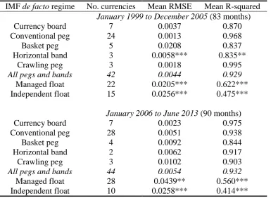
instructions, rather than a statistical algorithm.4 Table 1 shows the means for each IMF de
facto regime, and whether the mean is significantly different from the mean for a
conventional peg. The top panel of Table 1 refers to the earlier period and the bottom panel
to the later period.
What emerges quite clearly is that floats look different from pegs. Pegs tend to have
RMSEs below or close to 0.01, whereas for independent floats the RMSE tends to be above
0.02, and the average in each period is above 0.025. This pattern is mirrored in the
R-squareds. For independent floats the R-squared averages below 0.5 in each period. For pegs
of any kind, the average R-squared is always greater than 0.8, and in most cases considerably
closer to one than that. For pegs and bands as a whole, the average RMSE is 0.0044 in
1999-2005 and 0.0055 in 2006-13, and the average R-squared is 0.93 in each period. Managed
floats have an average RMSE of 0.0205 in 1999-2005 and 0.0245 in 2006-13, with average
R-squareds of 0.622 and 0.630 respectively. Moreover the statistics for managed and
independent floats are significantly different from those for conventional pegs, whereas the
4 The details are given in the IMF’s Annual Report on Exchange Arrangements and Exchange Restrictions. For
statistics for other types of pegs and bands are not, which provides some justification for a
[image:9.595.108.494.237.519.2]binary peg/float distinction.
Table 1. Regression statistics by IMF de facto regime
IMF de facto regime No. currencies Mean RMSE Mean R-squared
January 1999 to December 2005 (83 months)
Currency board 7 0.0037 0.870
Conventional peg 24 0.0013 0.968
Basket peg 5 0.0208 0.837
Horizontal band 3 0.0058*** 0.835**
Crawling peg 3 0.0018 0.995
All pegs and bands 42 0.0044 0.929
Managed float 22 0.0205*** 0.622*** Independent float 15 0.0256*** 0.475***
January 2006 to June 2013 (90 months)
Currency board 7 0.0023 0.975
Conventional peg 28 0.0051 0.938
Basket peg 4 0.0092 0.844
Horizontal band 2 0.0062 0.917
Crawling peg 3 0.0102 0.903
All pegs and bands 44 0.0054 0.932
Managed float 28 0.0439** 0.560*** Independent float 10 0.0258*** 0.414*** Notes. The statistics refer to the estimation of equation (4) for each currency. Currencies for which the IMF de facto classification records a regime
change are omitted. *,**,***: significantly different from a conventional peg at the 10, 5 and 1% levels respectively. The categories are as follows.
Currency Board: officially announced as such. Conventional peg: peg to a single currency with ±1% variation. Basket Peg: peg to a basket of
This difference in means is encouraging but not necessarily compelling. It does not tell us
how much overlap there is between the distributions. For example the high average RMSE of
0.0208 for the five basket pegs in the 1999-2005 period suggests that one or two of them may
look quite similar to floats according to these statistics. Indeed that is the case: the Libyan
dinar has an RMSE of 0.081 and an R-squared of 0.021 in that period. A particular issue is
the devaluation of a pegged currency. This is not a regime change, but in the regression it
would produce a large residual for that month. This would raise the RMSE and reduce the
R-squared, and could distort the other coefficients, as we show by an example in the next
section.
A symptom of one or more devaluations should be a distinctive pattern of residuals.
In the event of a devaluation, positive residuals (representing a depreciation relative to the
Swiss franc that is not explained by movements in the US dollar or the euro against the Swiss
franc) should be relatively infrequent but occasionally large, and negative residuals should be
on average much smaller but much more numerous. In other words, the residuals in this case
should be markedly positively skewed. For genuine floats, we do not expect the residuals to
be skewed in this way. In fact in the sample shown in Table 1, skewness never exceeds two
in absolute value for independent floats, but quite frequently does so for other regimes.
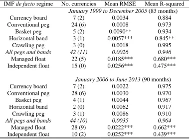
This suggests that the skewness of residuals can be used to identify months with
possible parity changes. For each of these months, a dummy variable that is equal to one for
that month only, and zero otherwise, can be added to the regression. The regression can then
be rerun, and the RMSE and R-squared re-examined. For pegs with occasional devaluations,
the resulting statistics should now be in the expected range for pegs; for floats that just
happened to have an usually large movement in one month, these statistics should be much
Table 2. Regression statistics by IMF de facto regime with a dummy for a single outlying month
IMF de facto regime No. currencies Mean RMSE Mean R-squared
January 1999 to December 2005 (83 months) Currency board 7 (2) 0.0034 0.884 Conventional peg 24 (6) 0.0008 0.973 Basket peg 5 (2) 0.0090** 0.934 Horizontal band 3 (1) 0.0057*** 0.845**
Crawling peg 3 (0) 0.0018 0.995
All pegs and bands 42 (11) 0.0026 0.946
Managed float 22 (5) 0.0185*** 0.680*** Independent float 15 (0) 0.0256*** 0.475***
January 2006 to June 2013 (90 months) Currency board 7 (2) 0.0022 0.975 Conventional peg 28 (6) 0.0030 0.970
Basket peg 4 (1) 0.0044 0.967
Horizontal band 2 (0) 0.0062 0.917 Crawling peg 3 (1) 0.0086 0.910
All pegs and bands 44 (10) 0.0035 0.964
Table 2 shows what happens if we include a dummy for a single outlying month in
cases where that dummy is highly significant. The procedure is as follows: if the sample is T
months in length, we run T extra regressions for each country, each with a dummy =1 in just
one month of the sample added to equation (4). If the highest F-statistic for the addition of a
dummy does not exceed 30 (equivalent to a t-statistic of √30 = 5.48), no dummies are added.
If at least one F-statistic does exceed 30, we include a dummy for the month which yields the
highest F-statistic, and no other dummies. The presumption is that there was a parity change
in that month. Then we use the statistics from this augmented regression instead of the
original one.5
In the case of Libya in the 1999-2005 period, the relevant month is January 2002, and
the inclusion of a dummy for that month reduces the RMSE from 0.081 to 0.025, and raises
the R-squared from 0.021 to 0.906. Thus the R-squared is now solidly in the range for a peg,
but the RMSE is still more typical of a float.
Table 2 shows that the dummy met the criterion for inclusion for eleven out of 42
pegs and bands in 1999-2005, and for seven out of 44 in 2006-13. The dummy was also
included for five out of 22 managed floats in the first period, and for six out of 28 managed
floats in the second, implying a significant parity change. The dummy never met the
criterion for inclusion for independent floats. The inclusion of the dummy reduces the
average RMSE for managed floats from 0.0205 to 0.0185 in 1999-2005, and from 0.0245 to
0.0230 in 2006-13. The R-squared for managed floats is 0.680 in the early period and 0.671
in the later period, compared with 0.622 and 0.630 respectively in Table 1. The average
RMSE for all pegs and bands in Table 2 is 0.0026 in 1999-2005 and 0.0031 in 2006-13,
compared with 0.0044 and 0.0055 respectively in Table 1, so the proportionate reduction in
RMSE from the inclusion of the dummies is greater for pegs and bands than for managed
5 A sample of twelve observations is too short to apply most standard tests for a structural break, but Monte
floats. The 1999-2005 average R-squared for all pegs and bands rises from 0.929 in Table 1
to 0.941 in Table 2, and the 2006-13 average R-squared for all pegs and bands rises from
0.942 to 0.971.
Overall, these results suggest that a search for outlying residuals in equation (4)
should enable pegs with occasional devaluations to be distinguished from genuine floats.
Managed floats are difficult to evaluate in general, because their behaviour depends
very much on how they are managed. As we shall show later, our methodology reveals that,
while some seem relatively lightly managed, others are quite close to a form of peg, usually
to the US dollar.
5
Some Examples
Table 3 gives some examples for pegs and bands (target zones wider than ±1%). In the first
column, the CFA franc from 1999 to 2005 is typical of an exact peg to a single currency: the
US dollar coefficient is zero, the euro coefficient is exactly 1.00, the R-squared is 1.00 and
the RMSE is 0.000. Typical of a slightly looser peg is China from 1999 to 2005, shown in
column (2): the US dollar coefficient is 1.001, with a t-statistic of 693, the euro coefficient is
0.015 and insignificant, the R-squared is 0.99 and the RMSE is 0.0023.
An example of a basket peg (Fiji 1999-2005) is given in column (3): all four
currencies have weights significantly different from zero, the R-squared is 0.98 and the
RMSE is 0.0035. In column (4), Tonga 2006-13 shows the difference between a peg and a
band. The US dollar, the Australian dollar and the New Zealand dollar all have significant
coefficients, but the R-squared is lower than for Fiji, at 0.85, and the RMSE is higher
(0.0099). In column (5), China 2006-13 is a good example of a crawling peg (in this case an
month, but the other statistics are typical of a peg, with an R-squared of 0.99 and an RMSE of
0.0041.
In all of these cases except China 1999-2005, the skewness of the residuals is small in
absolute terms, which suggests that there was no parity change during the period. In the case
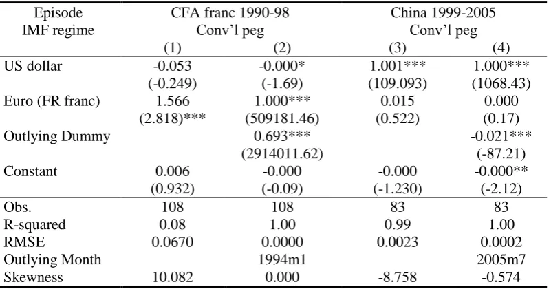
of China 1999-2005, skewness is -8.76, which indicates an appreciation at some date. Table
4 shows the effects of introducing a dummy for an outlying month for two cases: the CFA
franc, which was devalued by a very large amount in January 1994, from January 1990 to
December 1998, and China 1999-2005. It can be seen that, for the CFA franc, the January
1994 episode greatly affects the results: without the dummy variable for that month (column
1), the R-squared is only 0.08, and the RMSE is extremely high, at 0.0670. Even the French
franc coefficient is distorted, at 1.566 rather than 1.00. Only the residual skewness of 10.08
indicates that this is the effect of one or more large devaluations rather than floating. Once
the January 1994 dummy is included (column 2), the fit is perfect and the French franc
coefficient is exactly one.
In the case of China 1999-2005, introducing a dummy for July 2005 (column 4 of
Table 4) reduces skewness from -8.76 to -0.58, even though the estimated appreciation in that
Table 3. Some examples of pegs and bands
Episode CFA franc 1999-2005 China 1999-2005 Fiji 1999-2005 Tonga 2006-13 China 2006-13 IMF regime Conv’l peg Conv’l peg Basket peg Band Crawling peg
(1) (2) (3) (4) (5)
US dollar 0.000 1.001*** 0.298*** 0.515*** 0.957***
(0.83) (693) (18.0) (12.9) (57.6)
Euro 1.00*** 0.015 0.122** -0.094 0.031
(28413) (0.97) (2.31) (-1.03) (1.43)
AU dollar 0.331*** 0.173***
(16.9) (3.48)
NZ dollar 0.210*** 0.235***
(8.92) (4.88)
Constant -0.000 -0.000 -0.000 -0.000 -0.003*** (-0.00) (-1.20) (-0.36) (-0.26) (64.84)
Obs. 83 83 83 90 90
R-squared 1.00 0.99 0.98 0.85 0.99
RMSE 0.0000 0.0023 0.0035 0.0099 0.0041
Skewness 0.303 -8.758 0.408 -0.963 -0.697
Notes. The table refers to equation (4), with the monthly change in the log of the number of currency units per Swiss franc as the dependent variable. Figures in parentheses are t-statistics. *, **, *** denote significant at 10, 5 and 1% respectively. For 1990-98 the French franc is used in place of the euro.
Table 4. Introducing a dummy for a single outlying month
Episode CFA franc 1990-98 China 1999-2005
IMF regime Conv’l peg Conv’l peg
(1) (2) (3) (4)
US dollar -0.053 -0.000* 1.001*** 1.000***
(-0.249) (-1.69) (109.093) (1068.43)
Euro (FR franc) 1.566 1.000*** 0.015 0.000
(2.818)*** (509181.46) (0.522) (0.17)
Outlying Dummy 0.693*** -0.021***
(2914011.62) (-87.21)
Constant 0.006 -0.000 -0.000 -0.000**
(0.932) (-0.09) (-1.230) (-2.12)
Obs. 108 108 83 83
R-squared 0.08 1.00 0.99 1.00
RMSE 0.0670 0.0000 0.0023 0.0002
Outlying Month 1994m1 2005m7
Skewness 10.082 0.000 -8.758 -0.574
[image:15.595.100.501.488.698.2]Table 5 shows some examples of floats, all from 2006-13. In the first two columns,
Japan and Brazil are both classified as independent floats. For Japan the R-squared is 0.53
and the RMSE is 0.0274. For Brazil the R-squared is very low, at 0.19, and the RMSE is
0.0397. Skewness is 0.600 and 1.023 respectively, so not particularly high. Japan has a
surprisingly high US dollar coefficient, at 0.885, but a negative euro coefficient.6 Brazil has
significant positive coefficients for both (0.348 for the US dollar and 0.564 for the euro).
The remaining four columns of Table 5 are all examples of managed floats. India
looks very similar to the independent floats: low R-squared (0.47), high RMSE (0.0233) and
low skewness (0.074). The US dollar and euro coefficients are significant, but overall the
management appears to be quite light: the exchange rate displays much more variation than
under a peg. Kenya shows a similar pattern (R-squared of 0.12, RMSE of 0.0309 and
skewness of 0.697), but only the euro coefficient is significant, and the US dollar coefficient
is quite low. The last two columns show two cases where the managed float appears more
like a target zone for the exchange rate against the US dollar. In the case of Bangladesh, the
US dollar coefficient is 0.996, the R-squared is 0.88 and the RMSE is 0.0126 – much closer
to the peg range than one would expect for a float. Jamaica is essentially similar, with a US
dollar coefficient of 0.913, an R-squared of 0.89 and an RMSE of 0.0113. For Jamaica there
is also a marked trend depreciation, with a significant intercept term of 0.5% per month.
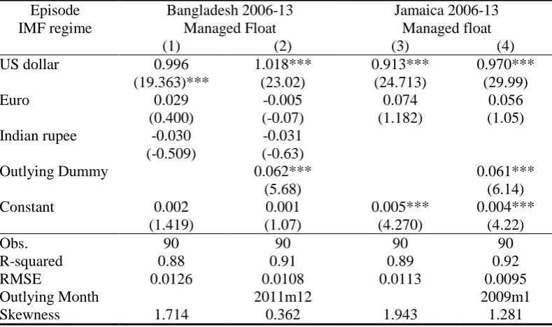
Table 6 shows that in both of these last two cases there seems to have been an
outlying month with a devaluation of about 6% (December 2011 for Bangladesh and January
2009 for Jamaica). Inclusion of the dummy makes their attachment to the US dollar look
even stronger.
Table 5. Some examples of independent and managed floats
Episode: Japan 2006-13 Brazil 2006-13 India 2006-13 Kenya 2006-13 Bangladesh 2006-13 Jamaica 2006-13 IMF regime Indep’t
Float Indep’t float Managed float Managed float Managed Float Managed float
(1) (2) (3) (4) (5) (6)
US dollar 0.885*** 0.348*** 0.530*** 0.158 0.996*** 0.913*** (9.88) (2.68) (6.96) (1.57) (19.363) (24.713) Euro -0.365** 0.564** 0.363*** 0.419** 0.029 0.074
(-2.40) (2.56) (2.80) (2.44) (0.400) (1.182) Indian
rupee -0.030
(-0.509)
Constant -0.001 0.000 0.004 0.004 0.002 0.005***
(-0.23) (0.09) (1.59) (1.08) (1.419) (4.270)
Obs. 90 90 90 90 90 90
R-squared 0.53 0.19 0.47 0.12 0.88 0.89
RMSE 0.0274 0.0397 0.0233 0.0309 0.0126 0.0113
Skewness 0.600 1.023 0.074 0.697 1.714 1.943
Notes. See notes to Table 3.
Table 6. Introducing a dummy for a single outlying month
Episode Bangladesh 2006-13 Jamaica 2006-13
IMF regime Managed Float Managed float
(1) (2) (3) (4)
US dollar 0.996 1.018*** 0.913*** 0.970***
(19.363)*** (23.02) (24.713) (29.99)
Euro 0.029 -0.005 0.074 0.056
(0.400) (-0.07) (1.182) (1.05)
Indian rupee -0.030 -0.031
(-0.509) (-0.63)
Outlying Dummy 0.062*** 0.061***
(5.68) (6.14)
Constant 0.002 0.001 0.005*** 0.004***
(1.419) (1.07) (4.270) (4.22)
Obs. 90 90 90 90
R-squared 0.88 0.91 0.89 0.92
RMSE 0.0126 0.0108 0.0113 0.0095
Outlying Month 2011m12 2009m1
Skewness 1.714 0.362 1.943 1.281
[image:17.595.103.498.438.672.2]6
The Choice of Numeraire
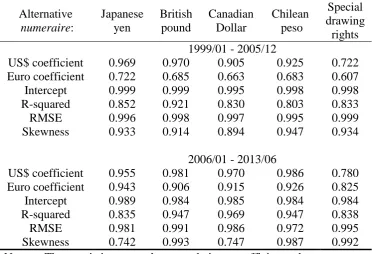
How much difference does the choice of numeraire make? Table 7 shows the correlation of
various regression statistics using other independently floating currencies as alternative
numeraires to the Swiss franc. The correlations are generally high. The R-squared, RMSE
and skewness always have correlations above 0.8, and in more than half the cases above 0.9.
The correlations for the intercept coefficient are particularly high, always exceeding 0.95.
The correlations for the US dollar coefficient always exceed 0.9, except in the case of the
SDR, for which the correlation is 0.722 in 1999-2005 and 0.760 in 2006-13. These lower
correlations no doubt reflect the weight of the US dollar in the SDR basket. For the euro
coefficients, the correlations are also lower for the SDR than for the other currencies,
although to a lesser degree, probably because the weight of the euro in the SDR basket is less
than that of the US dollar. For the euro coefficient, there is a marked difference between the
two periods. In 2006-13 the euro coefficient correlations for currencies other than the SDR
always exceed 0.9, whereas in 1999-2005 they lie in the range 0.66 to 0.73. This may reflect
the fact that the Swiss franc was particularly stable against the euro in this period, making the
Table 7. Correlations between statistics with different numeraires Alternative numeraire: Japanese yen British pound Canadian Dollar Chilean peso Special drawing rights 1999/01 - 2005/12
US$ coefficient 0.969 0.970 0.905 0.925 0.722 Euro coefficient 0.722 0.685 0.663 0.683 0.607 Intercept 0.999 0.999 0.995 0.998 0.998 R-squared 0.852 0.921 0.830 0.803 0.833 RMSE 0.996 0.998 0.997 0.995 0.999 Skewness 0.933 0.914 0.894 0.947 0.934
2006/01 - 2013/06
US$ coefficient 0.955 0.981 0.970 0.986 0.780 Euro coefficient 0.943 0.906 0.915 0.926 0.825 Intercept 0.989 0.984 0.985 0.984 0.984 R-squared 0.835 0.947 0.969 0.947 0.838 RMSE 0.981 0.991 0.986 0.972 0.995 Skewness 0.742 0.993 0.747 0.987 0.992 Notes. The statistics are the correlation coefficients between two alternative versions of equation (4), estimated with either the Swiss franc or the currency listed at the top of the column as numeraire, and with the inclusion of a dummy for an outlying month if the criteria described in Section 4 are met.
Nevertheless it is vital that the numeraire currency should float relative to the anchor
currencies used in the regression, and therefore it is always wise to test the robustness of
results to alternative numeraires. It is also important to identify anchor currencies correctly.
If currency A is pegged to currency B, but currency B is omitted from the regression,
currency A will tend to appear to have a regime similar to currency B, which may not be a
peg.
7
What Are Managed Floats Doing?
Managed floats are a bit of a black box. Calvo and Reinhart (2002) suggested that many
floats tend to have quite low bilateral volatility against the US dollar. Slavov (2013) finds a
high degree of attachment to the US dollar amongst floating sub-Saharan African countries.
It seems likely that many managed floats are quite lightly managed, whilst others are
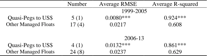
rather close to pegs of some kind. Suppose that we define managed floats that have an
RMSE of less than 0.015 (greater than virtually all pegs but less than virtually all independent
floats) and a regression coefficient of greater than 0.90 for the US dollar or the euro as a
quasi-peg to that currency. Then we find that, for the sample used in Tables 1 and 2, five out
of 22 managed floats in 1999-2005 and two out of 28 in 2006-13 qualify as quasi-pegs to the
US dollar. Thus a minority – but a diminishing minority – of managed floats appear to fall
into this category. Table 8 shows that the quasi-pegs also have much higher R-squareds than
is typical of other managed floats. The Table also shows that the difference in average
[image:20.595.89.509.473.588.2]RMSE and average R-squared is significant at the one percent level in each case.
Table 8. Different Types of Managed Floats
Number Average RMSE Average R-squared 1999-2005
Quasi-Pegs to US$ 5 (1) 0.0080*** 0.924***
Other Managed Floats 17 (4) 0.0217 0.608
2006-13
Quasi-Pegs to US$ 4 (1) 0.0132*** 0.861***
Other Managed Floats 24 (8) 0.0237 0.629
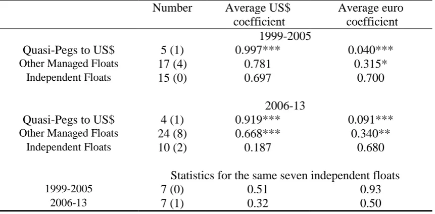
A separate question is whether even managed floats that are not quasi-pegs to the US
dollar are managed with particular attention to the bilateral rate against the US dollar. This
question can be addressed by comparing the US dollar coefficients of these managed floats
with those of independent floats (see Table 9). In the 1999-2005 period, the average US dollar coefficient of “other” managed floats is 0.781, which is slightly higher than the average
of 0.697 for independent floats, but the difference is not statistically significant. In 2006-13,
by contrast, the average US dollar coefficient of “other” managed floats is still quite high, at
0.668, wheareas the average for independent floats is much lower, at 0.187, and the
difference is statistically significant at the one percent level. The euro coefficients are very
similar across the two periods for each group (0.315 and 0.340 for “other” managed floats;
0.700 and 0.680 for independent floats), but much lower for independent floats, although the
difference is only significant at the five percent level for the 2006-13 period. Of course
geographical factors may be involved here, as we investigate below.
The bottom panel of Table 9 shows the average coefficients for the seven currencies
that were independent floats in the IMF de facto classification throughout the 1999-2013
period. The difference between the US dollar coefficients in the two periods is now much
smaller, but a large difference now appears between the euro coefficients in the two periods.
Considerable volatility in the coefficients of equation (4) is to be expected for genuinely
Table 9. Average US$ and Euro Coefficients of Different Types of Floats
Number Average US$ coefficient
Average euro coefficient 1999-2005
Quasi-Pegs to US$ 5 (1) 0.997*** 0.040***
Other Managed Floats 17 (4) 0.781 0.315*
Independent Floats 15 (0) 0.697 0.700
2006-13
Quasi-Pegs to US$ 4 (1) 0.919*** 0.091***
Other Managed Floats 24 (8) 0.668*** 0.340**
Independent Floats 10 (2) 0.187 0.680
Statistics for the same seven independent floats
1999-2005 7 (0) 0.51 0.93
2006-13 7 (1) 0.32 0.50
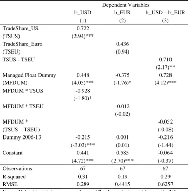
We now investigate the relationship between the US dollar coefficients and euro coefficients of “other” managed floats and independent floats and trade flows with the United
States and the Euro Area. One would expect that, where trade flows with a region are higher, that region would have a greater weight in a country’s effective exchange rate, and a higher
coefficient in equation (4). Table 10 shows that this is true, although the standard errors of
the trade coefficients are quite large, which is understandable in the case of floating
currencies. The coefficient of the US dollar increases significantly with trade flows to and
from the United States as a share of the country’s total trade (column (1)). The effect is
absent for “other” managed floats, although the difference in coefficients is not significant at
the 5% level. In column (2) the effect is smaller for the euro coefficients, and not statistically
significant. In column (3) (the difference between the US dollar and the euro coefficients)
the effect is almost as large as for the US dollar coefficient alone, and significant at the 5% level. In columns (2) and (3) the trade coefficient is only very slightly smaller for “other”
managed floats than for independent floats.
The managed float dummy in Table 10 tells us the estimated difference in coefficients between “other” managed floats and independent floats for given trade shares. If floats are
managed with more of an eye to the US dollar exchange rate and less to the euro exchange
rate, we would expect to see positive coefficients for this dummy in columns (1) and (3), and
a negative coefficient in column (2). This is exactly what we observe: the positive
coefficients in columns (1) and (3) have t-statistics that exceed four. The negative coefficient
in column (2) is only significant at the 10% level but almost as large in absolute value as that
in column (1). These results confirm the suggestion of Bleaney and Tian (2012) and Slavov
Table 10. Coefficients and Trade Shares for Different Types of Floats Dependent Variables
b_USD b_EUR b_USD – b_EUR
(1) (2) (3)
TradeShare_US 0.722
(TSUS) (2.94)***
TradeShare_Euro 0.436
(TSEU) (0.94)
TSUS - TSEU 0.710
(2.17)**
Managed Float Dummy 0.448 -0.375 0.728
(MFDUM) (4.05)*** (-1.76)* (4.12)***
MFDUM * TSUS -0.928
(-1.80)*
MFDUM * TSEU -0.012
(-0.02)
MFDUM * -0.052
(TSUS – TSEU) (-0.08)
Dummy 2006-13 -0.215 0.001 -0.216
(-3.03)*** (0.01) (-1.44)
Constant 0.441 0.585 -0.064
(4.72)*** (2.70)*** (-0.37)
Observations 67 67 67
R-squared 0.31 0.19 0.29
RMSE 0.289 0.4415 0.6257
8
Generating Annual Measures of Exchange Rate Flexibility
It is often useful to have an annual measure of exchange rate flexibility, or an annual
classification of exchange rate regimes, in order to assess how macroeconomic variables such
as growth, inflation and fiscal balances vary across regimes, to capture trends in regime
choice over time, or simply to provide a comparison with earlier classification schemes that
are organized by calendar year. The main issue for any regression method applied to a
relatively short period is the loss of degrees of freedom. Applied to twelve monthly changes,
equation (4) would have only nine degrees of freedom (fewer if extra potential anchor
currencies are included), and only eight once a parity change in one month is allowed for.
In order to generate an annual index of exchange rate flexibility for each country-year
observation, we adopt the following algorithm.
1) Estimate equation (4) for the twelve monthly exchange rate changes in the year,
adding potential anchor currencies to the US dollar and the euro as appropriate.
2) Add a dummy for January to the regression, then replace that with a dummy for
February, and so on. Record the lowest of these twelve RMSEs as the index of
exchange rate flexibility.
We have calculated this index for all years from 1970 to 2014 for three different
numéraire currencies (the Swiss franc, the Japanese yen and the British pound), and the data
are available in the online appendix.7 The distribution of the index is shown in Figure 1. It is
unimodal with a long right tail, reflecting the fact that floats vary considerably in their degree
of exchange rate volatility.
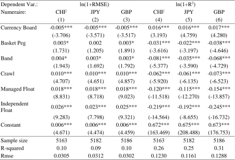
Table 11 shows regressions of two measures of exchange rate flexibility (the RMSE and
the R-squared) on the IMF classification categories for three numéraire currencies: the Swiss
franc, the Japanese yen and the British pound. It is particularly important to check other
numéraires, since the Swiss franc was not allowed to float freely for a period (from
September 2011 to January 2015). The results show that practically every category is
significantly different from a conventional peg, and in the expected direction, with only a
hard peg having a lower RMSE and a higher R-squared. Moreover the coefficient signs for
the R-squared are always the opposite of the signs for the RMSE. It is also reassuring that
the results are similar for the different numeraires.
Table 12 shows a similar regression for the Reinhart-Rogoff classification, which does
not identify hard pegs as a separate category, so all the coefficients in the RMSE regression
are positive, and all those in the R-squared regression are negative. “Freely falling” is a
special category for high-inflation economies, so it is not surprising that this category shows
even greater volatility than free floats.
Both tables suggest a fairly high correlation between our exchange rate flexibility
Table 11. Annual exchange rate flexibility measures and the IMF de facto classification (1980-2012)
Dependent Var.: ln(1+RMSE) ln(1+R2)
Numeraire: CHF JPY GBP CHF JPY GBP
(1) (2) (3) (4) (5) (6)
Currency Board -0.005*** -0.005*** -0.005*** 0.016*** 0.016*** 0.017*** (-3.706) (-3.571) (-3.517) (3.193) (4.759) (4.280) Basket Peg 0.003* 0.002 0.003* -0.031*** -0.022*** -0.038***
(1.731) (1.205) (1.891) (-3.616) (-3.197) (-4.646)
Band 0.004* 0.003* 0.003* -0.081*** -0.035*** -0.068***
(1.943) (1.692) (1.792) (-5.377) (-3.590) (-4.729) Crawl 0.010*** 0.010*** 0.010*** -0.062*** -0.061*** -0.073***
(4.707) (4.651) (4.857) (-5.920) (-6.135) (-6.523) Managed Float 0.018*** 0.018*** 0.018*** -0.120*** -0.115*** -0.154***
(8.831) (8.718) (9.023) (-11.518) (-12.270) (-13.857) Independent
Float 0.026*** 0.023*** 0.025*** -0.219*** -0.192*** -0.245*** (9.283) (7.798) (9.321) (-14.564) (-8.655) (-16.732) Constant 0.006*** 0.006*** 0.006*** 0.672*** 0.675*** 0.673*** (4.671) (4.474) (4.459) (163.469) (208.488) (176.753)
Sample size 5163 5182 5186 5163 5182 5186
R-squared 0.10 0.09 0.10 0.26 0.25 0.31
Rmse 0.0305 0.0312 0.0302 0.1230 0.1161 0.1288
Table 12. Annual exchange rate flexibility measures and the Reinhart-Rogoff classification (1970-2011)
Dependent Var.: ln(1+RMSE) ln(1+R2)
Numeraire: CHF JPY GBP CHF JPY GBP
(1) (2) (3) (4) (5) (6)
Crawl (±2%) 0.007*** 0.007*** 0.007*** -0.058*** -0.046*** -0.059*** (11.192) (11.594) (11.344) (-9.623) (-9.635) (-9.160) Band (±2 to 5%)
or 0.012*** 0.011*** 0.011*** -0.110*** -0.086*** -0.109*** Managed Float (11.278) (12.167) (11.675) (-9.706) (-9.705) (-9.407) Free Float 0.032*** 0.027*** 0.033*** -0.251*** -0.271*** -0.288***
(5.514) (3.923) (5.664) (-10.887) (-5.343) (-12.375) Freely Falling 0.056*** 0.057*** 0.055*** -0.184*** -0.195*** -0.189*** (10.199) (10.104) (10.165) (-11.590) (-11.672) (-10.753) Dual Currency 0.011** 0.011** 0.011** -0.049*** -0.052*** -0.088*** (2.258) (2.280) (2.215) (-3.121) (-2.815) (-2.626) Constant 0.002*** 0.002*** 0.002*** 0.677*** 0.677*** 0.666***
(5.907) (7.105) (5.757) (364.281) (418.373) (200.563)
Sample size 5524 5668 5676 5524 5668 5676
R-squared 0.20 0.22 0.21 0.21 0.23 0.20
Rmse 0.0293 0.0272 0.0273 0.1241 0.1184 0.1384
Notes. Estimation method: pooled OLS. The omitted category is a peg within a ±2% band. Regressions exclude the observations for USD, EUR (1999 onwards), FRF (up to 1998), DEM(up to 1998), and the numéraire currency. Standard errors are clustered for each country and t-statistics are in parentheses. Rmse is the root mean square error of the regression. The categories are as follows. Managed Float: residual category. Free Float: more than 20% of the monthly changes in the log of the exchange rate against every reference currency exceed 0.02. Freely Falling: rapid depreciation and high inflation. Duel Currency: a parallel exchange rate exists but data are absent (if parallel market rate data exist, the classification is based on them).
9
Conclusions
A simple and reliable regression method is used to generate an index of exchange rate
flexibility that, if desired, may be converted into a binary classification of exchange rate
regimes as in Bleaney and Tian (2014). The method is not data-intensive and could easily be
applied by other researchers. Monthly exchange rate movements of a currency against a
floating numeraire currency are regressed on movements of the euro and the US dollar
against the numeraire currency. Where relevant, other potential anchor currencies are added
numeraire (except that the SDR tends to be misleading because of its correlation with the
anchor currencies). The thorny question of distinguishing floats from pegs with occasional
parity changes can be addressed by examining the skewness of residuals; floats have
relatively symmetric residuals whereas pegs with occasional parity changes do not. The
procedure can be repeated with outlying observations dummied out to distinguish pegs with
parity changes from genuine floats. A useful by-product of this procedure is that it also
distinguishes “fixed” pegs (those without parity changes) from “variable” pegs (those with
parity changes).
Managed floats have become increasingly popular amongst emerging markets and
developing countries in the 21st century. In a small but diminishing minority of cases, our
results show that these are quasi-pegs to the US dollar, often with slightly wider target zones
than announced pegs. An increasing proportion of managed floats has similar volatility to
independent floats, but even these have a tendency to track the US dollar.
The method can be used to generate an annual measure of flexibility, which shows a
strong peak at relatively low levels of flexibility, and a long right tail (for the RMSE; for the
R-squared it is a long left tail). The annual index displays a satisfactory degree of agreement
with other regime classifications, but is richer in information, so it would be interesting to use
it in testing, for example, whether there is a significant correlation between exchange rate
flexibility and macroeconomic performance.
The index has several limitations. One is that, particularly for floating currencies, it
may vary considerably from period to period, particularly if measured over relatively short
periods such as a year. For example, the index for the UK in the 21st century varies from a
minimum of 0.0095 in 2006 to a maximum of 0.0319 in 2008. High-inflation economies are
likely to have high values whether they are genuinely floating or pegged with frequent
would be interesting to see how the index correlates with macroeconomic outcomes; this is a
topic that we leave to further research.
Acknowledgement
The authors wish to thank two anonymous referees for extremely helpful comments on an earlier draft of this paper. Any errors that remain are of course the authors’ responsibility.
References
Bénassy-Quéré, A., B. Coeuré and V. Mignon (2006), On the identification of de facto currency pegs, Journal of the Japanese and International Economies 20, 112-127
Bleaney, M.F. and M. Francisco (2007), Classifying exchange rate regimes: a statistical analysis of alternative methods, Economics Bulletin 6 (3), 1-6.
Bleaney, M.F. and M. Tian (2012), Currency networks, bilateral exchange rate volatility and the role of the US dollar, Open Economies Review 23 (5), 785-803
Bleaney, M.F. and M. Tian (2014), Classifying exchange rate regimes by regression methods, University of Nottingham School of Economics Discussion Paper no. 14/02
Bleaney, M.F., M. Tian and L. Yin (2015), De facto exchange rate regime classifications are better than you think, University of Nottingham School of Economics Discussion Paper no. 15/01
Calvo, G. and C.M. Reinhart (2002), Fear of floating, Quarterly Journal of Economics 117 (2), 379-408
Frankel, J. and S.-J. Wei (1995), Emerging currency blocs, in The International Monetary System: Its Institutions and its Future, ed. H. Genberg (Berlin, Springer)
Frankel, J. and S.-J. Wei (2008), Estimation of de facto exchange rate regimes: synthesis of the techniques for inferring flexibility and basket weights, IMF Staff Papers 55 (3), 384-416 Habermeier, K., A. Kokenyne, R. Veyrune and H. Anderson (2009), Revised system for the classification of exchange rate arrangements, IMF Working Paper no. 09/211
Levy-Yeyati, E. and F. Sturzenegger (2005), Classifying exchange rate regimes: deeds versus words, European Economic Review 49 (6), 1173-1193
Reinhart, C.M. and Rogoff, K. (2004), The modern history of exchange rate arrangements: a re-interpretation, Quarterly Journal of Economics 119 (1), 1-48
Rose, A.K. (2011), Exchange rate regimes in the modern era: fixed, floating and flaky, Journal of Economic Literature 49 (3), 652-672
Shambaugh, J. (2004), The effects of fixed exchange rates on monetary policy, Quarterly Journal of Economics 119 (1), 301-352
Slavov, S.T. (2013), De jure versus de facto exchange rate regimes in sub-Saharan Africa, Journal of African Economies 22 (5), 732-756