A
Supervised Anomaly Detection in Uncertain Pseudo-Periodic Data
Streams
JIANGANG MA, Victoria University LE SUN, Victoria University HUA WANG, Victoria University YANCHUN ZHANG, Victoria University UWE AICKELIN, The University of Nottingham
Uncertain data streams have been widely generated in many Web applications. The uncertainty in data streams makes anomaly detection from sensor data streams far more challenging. In this paper, we present a novel framework that supports anomaly detection in uncertain data streams. The proposed framework adopts an efficient uncertainty pre-processing procedure to identify and eliminate uncertainties in data streams. Based on the corrected data streams, we develop effective period pattern recognition and feature extraction techniques to improve the computational efficiency. We use classification methods for anomaly detection in the corrected data stream. We also empirically show that the proposed approach shows a high accuracy of anomaly detection on a number of real datasets.
Categories and Subject Descriptors: I.5.4 [Pattern recognition]: Applications General Terms: Design, Algorithms, Performance
Additional Key Words and Phrases: anomaly detection, uncertain data stream, segmentation, classification
1. INTRODUCTION
Data streams have been widely generated in many Web applications such as monitor-ing click streams [G ¨und ¨uz and ¨Ozsu 2003], stock tickers [Chen et al. 2000; Zhu and Shasha 2002], sensor data streams and auction bidding patterns [Arasu et al. 2003]. For example, in the applications of Web tracking and personalization, Web log entries or click-streams are typical data streams. Other traditional and emerging applications include wireless sensor networks (WSN) in which data streams collected from sensor networks are being posted directly to the Web. Typical applications comprise envi-ronment monitoring (with static sensor nodes) [Akyildiz et al. 2005] and animal and object behaviour monitoring (with mobile sensor nodes), such as water pollution detec-tion [He et al. 2012] based on water sensor data, agricultural management and cattle moving habits [CSIRO 2011], and analysis of trajectories of animals [Gudmundsson et al. 2007], vehicles [Zheng et al. 2010] and fleets [Lee et al. 2007].
Anomaly detection is a typical example of a data streams application. Here, anoma-lies or outliers or exceptions often refer to the patterns in data streams that deviate expected normal behaviours. Thus, anomaly detection is a dynamic process of finding abnormal behaviours from given data streams. For example, in medical monitoring ap-plications, a human electrocardiogram (ECG) (vital signs) and other treatments and
Correspondence author’s addresses: Yanchun Zhang, School of Computer Science, Fudan University, Shanghai 200433, China; and Centre for Applied Informatics, Victoria University, VIC, 3012, Australia
Permission to make digital or hard copies of part or all of this work for personal or classroom use is granted without fee provided that copies are not made or distributed for profit or commercial advantage and that copies show this notice on the first page or initial screen of a display along with the full citation. Copyrights for components of this work owned by others than ACM must be honored. Abstracting with credit is per-mitted. To copy otherwise, to republish, to post on servers, to redistribute to lists, or to use any component of this work in other works requires prior specific permission and/or a fee. Permissions may be requested from Publications Dept., ACM, Inc., 2 Penn Plaza, Suite 701, New York, NY 10121-0701 USA, fax+1 (212) 869-0481, or [email protected].
c
YYYY ACM 1533-5399/YYYY/01-ARTA $15.00 DOI:http://dx.doi.org/10.1145/0000000.0000000
measurements are typical data streams that appear in a form of periodic patterns. That is, the data present a repetitive pattern within a certain time interval. Such data streams are called pseudo periodic time series. In such applications, data arrives con-tinuously and anomaly detection must detect suspicious behaviours from the streams such as abnormal ECG values, abnormal shapes or exceptional period changes.
Uncertainty in data streams makes the anomaly detection far more challenging than detecting anomalies from deterministic data. For example, uncertainties may result from missing points from a data stream, missing stream pieces, or measurement er-rors due to different reasons such as sensor failures and measurement erer-rors from different types of sensor devices. This uncertainty may cause serious problems in data stream mining. For example, in an ECG data stream, if a sensor error is classified as abnormal heart beat signals, it may cause a serious misdiagnosis. Therefore, it is necessary to develop effective methods to distinguish uncertainties and anomalies, re-move uncertainties, and finally find accurate anomalies.
There are a number of related research areas to sensor data stream mining, such as data streams compression, similarity measurement, indexing and querying mech-anisms [Esling and Agon 2012]. For example, to clean and remove uncertainty from data, a method for compressing data streams was presented in [Douglas and Peucker 1973]. This method uses some critical points in a data stream to represent the original stream. However, this method cannot compress uncertain data streams efficiently be-cause such compression may result in an incorrect data stream approximation and it may remove useful information that can correct the error data.
This paper focuses on anomaly detection in uncertain pseudo periodic time series. A pseudo periodic time series refers to a time-indexed data stream in which the data present a repetitive pattern within a certain time interval. However, the data may in fact show small changes between different time intervals. Although much work has been devoted to the analysis of pseudo periodic time series [Keogh et al. 2005; Huang et al. 2014], few of them focus on the identification and correction of uncertainties in this kind of data stream.
In order to deal with the issue of anomaly detection in uncertain data streams, we propose a supervised classification framework for detecting anomalies in uncertain pseudo periodic time series, which comprises four components: a uncertainty iden-tification and correction component (UICC), a time series compression component (TSCC), a period segmentation and summarization component (PSSC), and a classifi-cation and anomaly detection component (CADC). First, UICC processes a time series to remove uncertainties from the time series. Then TSCC compresses the processed raw time series to an approximate time series. Afterwards the PSSC identifies the periodic patterns of the time series and extracts the most important features of each period, and finally the CADC detects anomalies based on the selected features. Our work has made the following distinctive contributions:
— We present a classification-based framework for anomaly detection in uncertain pseudo periodic time series, together with a novel set of techniques for segmenting and extracting the main features of a time series. The procedure of pre-processing un-certainties can reduce the noise of anomalies and improve the accuracy of anomaly detection. The time series segmentation and feature extraction techniques can im-prove the performance and time efficiency of classification.
— We conduct an extensive experimental evaluation over a set of real time series data sets. Our experimental results show that the techniques we have developed outper-form previous approaches in terms of accuracy of anomaly detection. In the experi-ment part of this paper, we evaluate the proposed anomaly detection framework on ECG time series. However, due to the generic nature of features of pseudo periodic time series (e.g. similar shapes and intervals occur in a periodic manner), we believe that the proposed method can be widely applied to periodic time series mining in different areas.
The structure of this paper is as follows: Section 2 introduces the related research work. Section 3 presents the problem definition and generally describes the proposed anomaly detection framework. Section 4 describes the anomaly detection framework in detail. Section 5 presents the experimental design and discusses the results. Finally, Section 6 concludes this paper.
2. RELATED WORK
We analyse the related research work from two dimensions: anomaly detection and uncertainty processing.
Anomaly detection in data streams:Anomaly detection in time series has var-ious applications in wide area, such as intrusion detection [Tavallaee et al. 2010], disease detection in medical sensor streams [Manning and Hudgins 2010], and bio-surveillance [Shmueli and Burkom 2010]. Zhang et al.[ling Zhang et al. 2009] designed a Bayesian classifier model for identification of cerebral palsy by mining gait sensor data (stride length and cadence). In stock price time series, anomalies exist in a form of change points that reflect the abnormal behaviors in the stock market and often re-peating motifs are of interest [Wilson et al. 2008]. Detecting change points has signif-icant implications for conducting intelligent trading [Jiang et al. 2011]. Liu et al. [Liu et al. 2010] proposed an incremental algorithm that detects changes in streams of stock order numbers, in which a Poisson distribution is adopted to model the stock orders, and a maximum likelihood (ML) method is used to detect the distribution changes.
The segmentation of a time series refers to the approximation of the time series, which aims to reduce the time series dimensions while keeping its representative fea-tures [Esling and Agon 2012]. One of the most popular segmentation techniques is the Piecewise Linear Approximation (PLA) based approach [Keogh et al. 2004; Qi et al. 2015], which splits a time series into segments and uses polynomial models to rep-resent the segments. Xu et al. [Xu et al. 2012] improved the traditional PLA based techniques by guaranteeing an error bound on each data point to maximally compact time series. Daniel [Lemire 2007] introduced an adaptive time series summarization method that models each segment with various polynomial degrees. To emphasize the significance of the newer information in a time series, Palpanas et al. [Palpanas et al. 2008] defined user-oriented amnesic functions for decreasing the confidence of older information continuously.
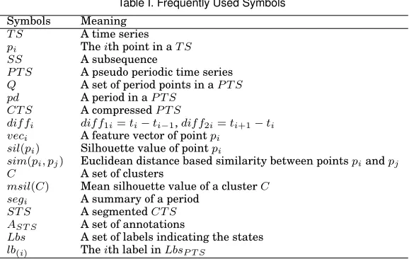
Table I. Frequently Used Symbols
Symbols Meaning T S A time series pi Theith point in aT S SS A subsequence
P T S A pseudo periodic time series Q A set of period points in aP T S pd A period in aP T S
CT S A compressedP T S
dif fi dif f1i=ti−ti−1,dif f2i=ti+1−ti veci A feature vector of pointpi
sil(pi) Silhouette value of pointpi
sim(pi, pj) Euclidean distance based similarity between pointspiandpj C A set of clusters
msil(C) Mean silhouette value of a clusterC segi A summary of a period
ST S A segmentedCT S AST S A set of annotations
Lbs A set of labels indicating the states lb(i) Theith label inLbsP T S
segmenting pseudo periods include an peak-point-based clustering method and valley-point-based method [Huang et al. 2014; an Tang et al. 2007]. These two methods may have very low accuracy when the processed time series have noisy peak points or have irregularly changed sub-sequences. Our proposed approach falls into the category of classification-based anomaly detection, which is proposed to overcome the challenge of anomaly detection in periodic data streams. In addition, our method is able to identify qualified segmentation and assign annotation to each segment to effectively support the anomaly detection in a pseudo periodic data streams.
Uncertainty processing in data streams: Most data streams coming from real-world sensor monitoring are inherently noisy and uncertainties. A lot of work has concentrated on the modelling of uncertain data streams [Aggarwal and Yu 2008; Ag-garwal 2009; Leung and Hao 2009]. Dallachiesa et al.[Dallachiesa et al. 2012] sur-veyed recent similarity measurement techniques of uncertain time series, and cate-gorized these techniques into two groups: probability density function based methods [Sarangi and Murthy 2010] and repeated measurement methods [Aßfalg et al. 2009]. Tran et al.[Tran et al. 2012] focused on the problem of relational query processing on uncertain data streams. However, previous work rarely focused on the detection and correction of the missing critical points for a discrete time series. In this work, we model a continuous time series as a discrete time series by identifying the critical points in a time series, and introduce a novel method of detecting and correcting the missing inflexions based on the angles between points.
3. PROBLEM SPECIFICATION AND FRAMEWORK DESCRIPTION
In this section, we first give a formal definition of the problems and then describe the proposed framework of detecting abnormal signals in uncertain time series with pseudo periodic patterns. The symbols frequently used in this paper are summarized in Table I.
3.1. Problem definition
Definition 3.1. Atime-series T S is an ordered real sequence:T S = (v1,· · ·, vn), wherevi,i∈[1, n], is a point value on the time series at timeti.
We use the form|T S|to represent the number of points in time seriesT S(i.e.,|T S|=
Definition 3.2. For time series T S, if SS(⊂ T S) comprises m consecutive points:
SS = (vs1,· · · , vsm), we say that SS is asubsequence of T S with length m,
repre-sented asSSvT S.
Definition 3.3. A pseudo periodic time series P T S is a time series P T S = (v1, v2,· · · , vn),∃Q={vp1,· · · , vpk|vpi ∈P T S, i ∈[1, k]}, that regularly separatesP T S
on the condition that
(1) ∀i∈[1, k−2], if41=|pi+1−pi|,42=|pi+2−pi+1|, then| 42− 41| ≤ξ1; whereξ1
is a small value.
(2) lets1= (vpi, v(pi)+1,· · · , vpi+1)vP T S, ands2 = (vpi+1, v(pi+1)+1,· · · , vpi+2)vP T S, thendsim(s1, s2) ≤ ξ2, wheredsim()calculates the dis-similarity betweens1 and
s2, and ξ2 is a small value. dsim()can be any dis-similarity measuring function
between time series, e.g., Euclidean distance.
In particular,vpi+1 ∈Qis called a period point.
An uncertainP T Sis aP T Shaving error detected data or missing points.
Definition 3.4. If pd v P T S, andpd = (vpi, v(pi)+1,· · ·, vpi+1),∀vpi ∈ Q, thenpd is
called aperiodof theP T S.
Definition 3.5. Anormal patternM of aP T Sis a model that uses a set of rules to describe a behaviour of a subsequenceSS, wherem=|SS|andm∈[1,|P T S|/2]. This behaviour indicates the normal situation of an event.
Based on the above definitions, we describe types of anomalies that may occur in a
P T S. There are two possible types of anomalies in aP T S: local anomalies and global
anomalies Given theP T Sin Definition 3.3, and a normal patternN = (v1,· · ·, vm)v
P T S, a local anomaly(L)is defined as:
Definition 3.6. AssumeL = (vl1,· · · , vln) v P T S,L is a local anomaly if either of
the two conditions in Definition 3.3 is broken (shown as below (1)), and at the same time satisfies the following two conditions (below (3)):
(1) 4N − 4L> ξ1ordsim(N, L)> ξ2;
(2) frequency ofL: f req(L) f req(N)andLdoes not happen in a regular sampling frequency.
(3) |L| |P T S|.
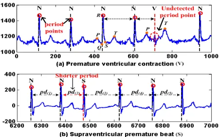
Example 3.7. Fig.1 shows two examples of pseudo periodic time series and their local anomalies. Fig.1(a) shows a premature ventricular contraction signal in an ECG stream. A premature ventricular contraction (PVC) [Levy and Pappano 2007] is per-ceived as a ”skipped beat”. It can be easily distinguished from a normal heart beat when detected by the electrocardiogram. From Fig.1(a), the QRS and T waves of a PVC (indicated by V) are very different from the normal QRS and T (indicated by N). Fig.1(b) presents an example of premature atrial contractions (PACs)[Folarin et al. 2001]. A PAC is a premature heart beat that occurs earlier than the regular beat. If we use the highest peak points as the period points, then a segment between two peak points is a period. From Fig.1, the second period (a PAC) is clearly shorter than the other periods.
3.2. Overview of the Anomaly Detection Framework for Uncertain Time Series Data
Fig. 1. Two examples of local anomaly in ECG time series
Fig. 2. Workflow of themitdbprocessing based on the proposed framework
and an anomaly detection and prediction component (ADPC). We explain the process of anomaly detection of the proposed framework using an example of the datasetmitdb. Fig.2 shows the processing progress of mitdb. First, the rawmitdb time series is an input to the UICC component. The TS1in Fig.2 shows a subsequence of the rawmitdb. The UICC identifies the inflexions (including missing inflexions) ofmitdb, and the raw
mitdbis transformed into an approximated time series that only consists of the
iden-tified inflexions (TS2in Fig.2). The TSCC component then further compresses the ap-proximatedmitdb. The TS3in Fig.2 shows the compressed time series (CT S) that is a compression of the subsequence in TS2. The PSSC component segments the time se-ries and assigns annotations to each segment. TS4in Fig.2 shows the segmented and annotatedCT Scorresponding to theCT Sin TS3. Finally, the ADPC component learns a classification model based on the segmented CT Sto detect abnormal subsequences in similar time series.
In the next section, we introduce the framework and its four components in detail.
4. ANOMALY DETECTION IN UNCERTAIN PERIODIC TIME SERIES 4.1. Uncertainty Identification and Correction: UICC
In this section, we introduce the procedure of eliminating uncertainties of a P T S
caused by non-captured key-points of a P T S, based on our previous work [He et al. 2013]. We first introduce the definition of key-points of a time series.
Definition 4.1. Given aP T S = (v1,· · · , vn), if a point, pi = v1 or vn, is a turning
point, thenpiis a key-point; or else, if6 pi =π−6 pjpipk and6 pi > , where6 pi is the angle between vectors−−→pjpi and−−→pipk,2≤j < i < k≤n,is a threshold,pj andpk are key-points, and for any pointpr, j < r < k,6 pr≤, thenpiis a key-point.
From the above definition, the core procedure to determine a pointpkas a key-point is based on the angles between−−−−→pk−1pk and−−−−→pkpk+1(i.e.,6 pk =π−6 pk−1pkpk+1), given
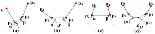
[image:6.612.195.422.92.233.2] [image:6.612.166.448.264.323.2]Fig. 3. (a)p2is a key-point. (b)pis a missing key-point. (c)p2 andp3are two key-points. (d)pk1andpk2
are two missing key-points, whilepis one deduced key-point.
the angles of all the other points between k−1 and k+ 1 are not larger than the threshold, thenpk is a key-point. However, ifpk is missing, we need to check at least four points: two key-points before and two key-points afterpkrespectively. Therefore, we generally check four consecutive points at the same time. Combined with Fig.3, the detailed process is described below:
Given four consecutive pointsp1=v1,p2=v2,p3=v3, andp4=v4, wherep1andp4
are key-points, and a small value→0, let6 p2=π−6 p1p2p3and6 p3=π−6 p2p3p4,
— If 6 p2 > , 6 p3 < , and there is no other point between p1 and p4, then p2 is a
key-point (see Fig.3(a));
— If6 p2< , and6 p3> , thenp3is a key-point;
— If6 p2> ,6 p3> , and6 p2+6 p3< π, then there may be a missing key-point. In this
case, it is also possible that both ofp2andp3are key-points. If we can find a missing
pointp=vat timet, that6 p=6 p2+6 p3≥2∗, then the pointpis more likely to be
a key-point betweenp2 andp3, as the larger6 pindicates the larger turning degree
of the time series at pointp. We deduce missing key-points by solving the equation
Q= |p2p|
sin(6 p3)
= |p3p| sin(6 p2)
, whereQ= |p2p3| sin(π−6 p2−6 p3)
, which can be written as:
Q2sin26 p
3= (v−v2)2+ (t−t2)2
Q2sin26 p
2= (v−v3)2+ (t−t3)2 (1)
If Equation (1) only has one solution, this solution is a key-point; if it has two solu-tions, we adopt the one on the line ofp1p2, i.e.,pin Fig.3(b) as a key-point; if it does
not have solution, pointp2andp3are key-points.
— If6 p2> ,6 p3> , and6 p2+6 p3> π, thenp2 andp3are both key-points (Fig.3(c)).
In addition, it is impossible that there are other missing points, say p, betweenp2
andp3, that6 p > .
— If more than one consecutive key-points are missing, the above method will only detect one missing point as an representation of all the missing key-points. For ex-ample, Fig.3(c) showspk12andpk22are two missing key-points, however, one virtual
key-pointp2based on the existing pointsp1,pk11,pk21, andp3are deduced.
Key-points capture the critical information and fill the missing information of a
P T S, hence, the detected key-points can be used to represent the raw P T S. In the
sequel sections, aP T Stypically refers to a series of key-points of the originalP T S.
4.2. Anomaly Detection in Corrected Time Series
[image:7.612.180.436.95.151.2]Fig. 4. AP T Sand one of itsCT Ss
the time series. The period points are the points that can regularly and consistently separate theP T Sbetter than the points in the other clusters.
The cluster quality validation mechanism is a silhouette-value based method, in which the cluster that have highest mean silhouette value will be assumed to have the best clustering pattern. To accurately conduct clustering, we introduce a feature vector for each inflexion of P T S, with the optimal intention that each point can be distinguished with others efficiently.
4.2.1. Time Series Compression: TSCC. To save the storage space and improve the cal-culation efficiency, the rawP T Swill first be compressed. In this work, we use the Dou-glas–Peucker (DP) [Hershberger and Snoeyink 1994] algorithm to compress a P T S, which is defined as: (1) use line segmentp1pnto simplify theP T S; (2) find the farthest pointpf fromp1pn; (3) if distanced(pf, p1pn)≤λ, whereλis a small value, andλ≥0, then theP T Scan be simplified byp1pn, and this procedure is stopped; (4) otherwise, recursively simplify the subsequences{p1,· · ·, pf}and{pf,· · ·, pn}using steps(1−3).
Definition 4.2. Given aP T S = (v1,· · · , vn), a compressed time series CT S of
P T Sis represented asCT S= (vc1,· · · , vcn)⊆P T S, where∀pci ∈CT Sis an inflexion,
and|CT S| |P T S|.
The feature vector of an inflexion is defined as:
Definition 4.3. A feature vector for a point pi ∈ P T S is a four-value vector
veci= (vdif f1i, vdif f2i, tdif f1i, tdif f2i), wherevdif f1i=vi−vi−1,vdif f2i =vi+1−vi,
tdif f1i=ti−ti−1, andtdif f2i=ti+1−ti.
Example 4.4. Fig.4 shows an example of a P T S and one of its compressed time seriesCT S. The value differencesvdif f1andvdif f2, and the time differenceswdif f1
andwdif f2are shown in Fig.4.
4.2.2. Period Segmentation and Summarization: PSSC.PSSC component identifies period points that separate theCT S into a series of periods, which is implemented by three steps: cluster points ofCT S, evaluate the quality of clusters based on silhouette value, and Segment and annotate periods. Details of these steps are given below.
[image:8.612.211.408.92.226.2]k-means++ is an improvement ofk-means by first determining the initial clustering centres before conducting the k-means iteration process. k-means is a classical N P -hard clustering method. One of its drawbacks is the low clustering accuracy caused by randomly choosing thekstarting points. The arbitrarily chosen initial clusters can-not guarantee a result converging to the global optimum all the time.k-means++ is proposed to solve this problem. K-mean++ chooses its first cluster center randomly, and each of the remaining ones is selected according to the probability of the point’s squared distance to its closest centre point being proportional to the squared distances of the other points. Thek-means++ algorithm has been proved to have a time complex-ity ofO(logk)and it is of high time efficiency by determining the initial seeding. For more details ofk-means++, readers can refer to [Arthur and Vassilvitskii 2007].
Step 2: Evaluate the quality of clusters based on silhouette value. We use the mean Silhouette value[Rousseeuw 1987] of a cluster to evaluate the quality of a cluster. The silhouette value can interpret the overall efficiency of the applied cluster-ing method and the quality of each cluster such as the tightness of a cluster and the similarity of the elements in a cluster. The silhouette value of a point belonging to a cluster is defined as:
Definition 4.5. Let points in P T S be clustered into k clusters: CCT S = {C1,· · ·, Cm,· · · , Ck}, k ≤ |CT S|. For any point pi = vi ∈ Cm, the silhouette value ofpiis
sil(pi) = b(pi)−a(pi)
max{a(pi), b(pi)} (2)
where a(pi) = M1−1P
pi,pj∈Cm,i6=jsim(pi, pj), M = |Cm| is the number of elements in
cluster m; b(pi) = min(M1−1
P
pi∈Cm,pj∈Ch,h6=msim(pi, pj)). sim(pi, pj) represents the
similarity betweenpiandpj.
In the above definition, sim(pi, pj) can be calculated by any similarity calculation formula. In this work, we adopt the Euclidean Distance as similarity measure, i.e.,
sim(pi, pj) =
p
(vi−vj)2+ (ti−tj)2, wheretiandtjare the time indexes of the points
pi andpj. From the definition,a(pi)measures the dissimilarity degree between point
piand the points in the same cluster, whileb(pi)refers to the dissimilarity betweenpi and the points in the other clusters. Therefore, a smalla(pi)and a largeb(pi)indicate a good clustering. As −1 ≤ sil(pi) ≤ 1, a sil(pi) → 1 means that a point pi is well clustered, while sil(pi) →+ 0 represents the point is close to the boundary between
clustersM andH, and sil(pi)< 0indicates that point pi is close to the points in the neighbouring clusters rather than the points in clusterM.
The mean value of the silhouette values of points is used to evaluate the quality of the overall clustering result: msil(CCT S) = |CT S1 |Ppi∈CT Ssil(pi). Similar to the
silhouette value of a point, themsil→1represents a better clustering.
After clustering, we need to choose a cluster in which the points will be used as pe-riod points for theCT S. The chosen cluster is calledperiod cluster. The points in the period cluster are the most stable points that can regularly and consistently separate
CT S. We use the mean silhouette value of each cluster to evaluate the efficiency of a single cluster, represented asmsil(Cm) = P
pi∈Cmsil(pi), where−1 ≤msil(Cm) ≤1,
ALGORITHM 1:Cluster quality validation
Input: (1)V ={veci|1≤i≤ |CT S|}, whereveci= (αi, dif f1i, dif f2i) (2) A set of point clusters:CCT S={Cm|1≤m≤k}
(3) Threshold valuesηandξ,0≤η, ξ≤1
Output: Period clusterCperid Calculatesil(pi)for∀pi∈CT S;
Calculate mean silhouette value:msil(CCT S);
ifmsil(CCT S)< ηthen
Cperid=N U LL; return;
end
Cperid=max(msil(Cm)) &msil(Cm)> ξfor∀Cm∈CCT S.
change the number of clusters. The last line indicates that the chosen period cluster is the one with highest mean silhouette values that is higher than a thresholdξ.
Step 3.Segmentation and annotation of periods. As mentioned in the previous sec-tion, a CT S can be divided into a series of periods by using the period points. Thus detecting a local anomaly in CT S means to identify an abnormal period or periods. In this section, we introduce a segmenting approach to extract the main and com-mon features of each period. The extracted information will be used as classification features that are used for model learning and anomaly detection. In addition, signal annotations (e.g., ’Normal’ and ’Abnormal’) are attached to each period based on the original labels of the correspondingP T S. We will first give the concept of a summary of a period.
Definition 4.6. Given a CTS that has been separated into D periods, a sum-mary of a period pdi = (vi1,· · · , vim),1 ≤ i ≤ D is a vector segi =
(hmin
i , tmini , hmaxi , tmaxi , himea, pminmaxi , pli), where hmini is the amplitude value of the point having minimum amplitude in periodi:hmin
i =min{vik; 1≤k≤m};t
min i is the time index of the point with minimum amplitude. If there are two points having the minimum amplitude, tmin
i is the time index of the first point.hmaxi = max{vik};t
max i is the first point with maximum amplitude;hmea
i = m1(
Pv
ik);p
minmax
i =|tmaxi −tmini |;
pli=tim−ti1.
We represent the segmented CT S as ST S = {seg1,· · · , segn}. Each period
corre-sponds to an annotationannindicating the state of the period. In this paper, we will only consider two states:normalandabnormal. Therefore, aST Sis always associated with a series of annotationsAST S={ann1,· · ·, annn}.
For the supervised pattern recognition model, the original P T S has a set of labels to indicate the states of the disjoint sub-sequences ofP T S, which are represented as
Lbs = {lb(1),· · · , lb(w)}, ∀lb(r) = {0N0(N ormal),0Ab0(Abnormal)},1 ≤ r ≤ w. However,
Lbs cannot be attached to the segmentations of the P T S directly because the peri-odic separation is independent from the labelling process. To determine the state of a segmentation, we introduce a logical-multiplying relation of two signals:
Rule 1.ann=⊗(0Ab0,0N0) =0 Ab0 andann=⊗(0N0,0N0) =0N0.
Assume a period covers a subsequence that is labelled by two signals, if there exists an abnormal behaviour in the subsequence, then based on rule 1, the behaviour of the segmentation of the period is abnormal; otherwise the period is a normal series. This label assignment rule can be extended to multiple labels: given a set of labels
Lbs = {lb1,· · ·, lbr}, if ∃lbj =0 Ab0,1 ≤ j ≤ r, the value ofLbsis0Ab0, represented as
ALGORITHM 2:Period annotation
Input: Periodpdi= (vi1,· · ·, vim),1≤i≤n; A series of labelsLbs= (lb1,· · ·, lbr);
Output: An annotatedpd0i;
t1i =N U LL: the time of the1stannotation in the period;
tendi =N U LL: the time of the last annotation in the period;
if∃lbjthatt(i−1)1≤tj−1≤t(i−1)m< ti1≤tj≤timthen
t1i =tj;
end
if∃lbk&ti1≤tk≤tim&t(i+1)1≤tk+1≤t(i+1)mthen
tendi =tk;
end
ift1i 6=N U LLktendi 6=N U LLthen
ift1i =N U LLthen
t1i =0N0
end
iftendi =N U LLthen
tendi = 0
N0
end
Lbs=Lbs{t1i,· · ·, tendi };
lbs=⊗(Lbs);
else
lbs=Lbs{t1
i+1};
end
Fig. 5. Segmentation and annotation of two periods
According to the above discussion, the annotation of a period pdi is determined by Algorithm 2.
Example 4.7. We present the segmentation and annotation of a period in Fig.5 to explain their processes more clearly. Fig.5 shows that pdi does not involve any label and the first label inpdi+1islb1=N, solbpdi =
0N0.lb
2is ’Ab’, hencepdi+1is annotated
as ’Ab’.
[image:11.612.102.504.92.518.2]Table II. ECG Datasets used in experiments
Datasets Abbr. #ofSamples AnomalyTypes #ofAbnor #ofNor
AHA0001 ahadb 899750 V 115 2162
SupraventricularArrhythmia800 svdb 230400 S & V 75 1846 SuddenCardiacDeathHolter30 sddb 22099250 V 38 5743 MIT-BIH Arrhythmia100 mitdb 650000 A & V 164 2526 MIT-BIH Arrhythmia106 mitdb06 650000 A & V 34 2239
MGH/MF Waveform001 mgh 403560 S & V 23 776
MIT-BIH LongTerm14046 ltdb 10828800 V 000 000
AF TerminationN04 aftdb 7680 NA NA NA
In the next section, we validate the proposed anomaly detection framework with vari-ous classification methods on the basis of different ECG datasets.
5. EXPERIMENTAL EVALUATION
Our experiments are conducted in four steps. The first step is to compress the raw ECG time series by utilizing the DP algorithm, and to represent each inflexion in the perceived CT Sas a feature vector (see Definition 4.4). Secondly, theK-means++ clustering algorithm is applied to the series of feature vectors of the CT S, and the clustering result is validated by silhouette values. Based on the mean silhouette value of each cluster, a period cluster is chosen and the CT S is periodically separated to a set of consistent segments. Thirdly, each segment is summarised by the seven fea-tures (see Definition 4.6). Finally, a normal pattern of the time series is constructed and anomalies are detected by utilizing classification tools on the basis of the seven features.
We validate the proposed framework on the basis of eight ECG datasets [Goldberger et al. 2000a], which are summarised in Table II where ’V’ represents Premature ven-tricular contraction, ’A’: Atrial premature venven-tricular, and ’S’: Supravenven-tricular pre-mature beat. Apart from theaf tdbdataset, each time series is separated into a series of subsequences that are labelled by the dataset provider. We give the number of ab-normal subsequences (’#ofAbnor’) and the number of ab-normal subsequences (’#ofNor’) of each time series in Table II.
Our experiment is conducted on a 32-bit Windows system, with 3.2GHz CPU and 4GB RAM. The ECG datasets are downloaded to a local machine using the WFDB toolbox [Silva and Moody 2014; Goldberger et al. 2000b] for32-bit MATLAB. We use the10-fold cross validation method to process the datasets.
The metrics used for evaluating the final anomaly classification results include: (1) Accuracy (acc):(T P +T N)/ Number of all classified samples;
(2) Sensitivity (sen):T P /(T P +F N); (3) Specificity (spe):T N /(F P +T N);
(4) Prevalence (pre):T P / Number of all samples.
(5) Fmeasure (fmea):2∗ precisionprecision+∗recallrecall, whererecall=sen,precision= T PT P+F P
T P = true positive,T N = true negative,F P = false positive, andF N = false negative. Details of the experiments are illustrated in the following sections.
5.1. Inflexion Detection and Time Series Compression
Table III. Decreasing monotonicity degree of six datasets in terms of the value ofandλ
ahadb svdb sddb mitdb mgh aftdb
100 100 100 100 100 100
λ 100 100 100 100 100 100
Fig. 6. Monotonically decreasing number of breakpoints in terms offor the inflexion detection procedure andλfor the DP algorithm
The monotonicity index is used to measure the monotonically decreasing or increas-ing trend of the number of break points when the values of scale parameters of a polygonal approximation algorithm are changed. For the inflexion detection algorithm and the DP algorithm, if the values of the scale parameters and λare increasing, the number of the produced breakpoints of the time series will be decreasing, and vice versa. The decreasing monotonicity index is defined asMD = (1−TT+
−)×100, and the
increasing monotonicity index isMI = (1−TT−
+)×100, whereT− =−
P
∀∆vi<0∆vi/hi, T+ =P∀∆vi>0∆vi/hi, andhi =
vi+vi−1
2 . Both ofMD andMI are in the range[0,100],
and their perfect scores are100.
We test the decreasing monotonicity degrees for the datasetsahadb,svdb,sddb,mitdb,
mgh, andaf tdbin terms of different values offor inflexion detection procedure and
λfor DP algorithm. For the inflexion detection procedure, we set= 1,2,3,4,5. Table III shows that the breakpoint numbers for the six datasets are perfectly decreasing in terms of the increasing, which can also be seen in Fig.6(a). For DP algorithm, we first fix= 1, and detect inflexions of the six time series. Based on the detected inflexions, we setλ = 5,10,15,20,25,30,35,40,45,50to conduct DP compression. From Table III and Fig.6(b), we can see that the numbers of breakpoints are also100%decreasing in terms of the increasingλ.
The break-point stability index is defined as the shifting degree of breakpoints when deleting increasing amounts from the beginning of a time series. We use the endpoint stability to test the breakpoint stability for fixed parameter settings : = 1 for the inflexion detection andλ= 10for the DP algorithm. The endpoint stability measure-ment is defined asS = (1−1
m
P
d
P
b sdb
ndld), wheremis the level number of deletion,dis
thedthlevel,sd
Table IV. Endpoint stability of six datasets and pertubations
ahadb svdb sddb mitdb mgh aftdb Shifting length 10000 10000 10000 10000 10000 100 S 100 99.8988 99.9955 99.9725 99.9348 99.9351
conduct the DP algorithm based on the new time series. The positions of the identified breakpoints in each running circle are compared with the positions of the breakpoints identified in the whole ahadb. From Table IV, we can see that each time series is of high stability (i.e. values of S) when conducting the uncertainty detection procedure and the DP algorithm with fixed scale parameters.
5.2. Compressed Time Series Representation
From the above testing (see Fig.6), we can see that when≥4, the number of detected inflexions of each time series is going to be0. Based on Fig.6, we set= 1andλ= 10 for inflexion detection and time series compression. We then compare three methods of period point representation: (1) inflexions in CT Sare represented by feature vectors (FV); (2) inflexions are represented by angles (Angle) of peak points [Huang et al. 2014]; (3) inflexions are represented by valley points (Valley) [an Tang et al. 2007]. Valley points are points in aP T S, which have values less than an upper bound value (represented asU).U is initially specified by users and will be updated as time evolves. The update procedure is defined asUb=α(P
N
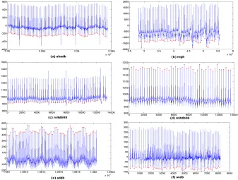
i=1Vi)/N, whereNis the number of past valley points and α is an outlier control factor that is determined and adjusted by experts. As stated by Tang et al.[an Tang et al. 2007], the best values of initial upper bound and α in ECG are50mmHg and 1.1. The perceived feature vector sets, angle sets, and valley point sets are passed to the next step in which points are clustered and the period points of theCT Sare identified. Each period is then segmented using the proposed segmentation method(see Definition 4.6). Finally, Linear Discriminant Analysis (LDA) and Naive Bayes(NB) classifiers are applied for sample classification and anomaly detection. Fig 7 shows the identified period points using the FV-based method for four datasets: ltdb, sddb,svdb andahadb. From Fig 7, we can see that for each dataset, the FV-based method successfully identifies a set of periodic points that can separate theCT Sin a stable and consistent manner.
Table V presents the silhouette values of clustering the inflexions in the CT Ss of seven time series, where column ’mean’ refers to the mean silhouette value of a dataset clustering, and the values in columns c(luster)1-6 are the mean silhouette values of each cluster after clustering a dataset. ’NAs’ in the sixth column means that the in-flexions in the corresponding datasets are clustered into five groups, which present the best clustering performance in this dataset. From Definition 4.5, we know that if the silhouette values in a cluster is close to 1, the cluster includes a set of points having similar patterns. On the other hand, if the silhouette values in a cluster are signifi-cantly different from each other or have negative values, the points in the cluster have very different patterns with each other or they are more close to the points in other clusters. Table V shows that for each of the seven datasets, the mean silhouette val-ues of the overall clustering result and each of the individual clusters are higher than 0.4(η = 0.4in algorithm 1). The best silhouette value of an individual cluster in each dataset is close to or higher than 0.9 (ξ = 0.8 in Algorithm 1). In addition, for each dataset, we select the points in the cluster with highest silhouette value as the period points. For example, for datasetahadb, points in cluster4are selected as period points.
Fig 8 presents the silhouette values of clustering the inflexions in theCT Ssofmitdb
and ltdb time series. From this figure, we can see that for both the mitdb and ltdb
clus-Fig. 7. Period point identification of four datasets based on feature vectors
Table V. Silhouette values of six datasets
Dataset Silhouette values
mean cluster1 (c1) c2 c3 c4 c5 c6
ahadb 0.8253 0.4479 0.8502 0.9824 0.9891 0.9381 NA svdb 0.6941 0.9792 0.6551 0.9703 0.5463 0.5729 0.959 sddb 0.772 0.6888 0.5787 0.965 0.9727 0.6971 0.7529 mitdb 0.9373 0.9877 0.7442 0.9898 0.9711 0.5854 0.3754 mitdb06 0.7339 0.7317 0.8998 0.609 0.8577 0.8669 NA
ltdb 0.9149 0.9164 0.8381 0.9739 0.9079 0.8975 NA mgh 0.8253 0.4479 0.8502 0.9824 0.9891 0.9381 NA
ters, and he values in each cluster are more similar to each other compared with the angle-based clustering. We also come to a similar conclusion by examining their mean silhouette values. The mean silhouette values of FV-based clustering formitdb (corre-sponding to Fig.8(a)) is0.9373, while the angle-based clustering (Fig.8(b)) is0.7461; and the mean values forltdbare0.9149and0.8155(Fig.8(c) and Fig.8(d)) respectively.
[image:15.612.153.465.406.492.2]Fig. 8. Silhouette value comparison between the feature vector based clustering method (FV-based) and the angle-based clustering method for themitdbandltdbdatasets
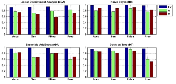
Fig. 9. Average performance comparison of four classifiers (LDA, NB, ADA, DT) based on feature vector based (FV), angle based (A) and valley point based (V) periodic separating methods
5.3. Evaluation of Classification Based on Summarized Features
This section describes the experimental design and the performance evaluation of clas-sification based on the summarized features. This experiment is conducted on seven datasets: ahadb,svdb, sddb,mitdb, mitdb06, mgh, andltdb. From the previous subsec-tions, we know that the seven time series have been compressed and the period seg-menting points have been identified (see Table V). The segments of each of the time series are classified by using three classification tools: Random Forest with 100 trees (RF), LDA and NB. We use matrices ofacc,sen,spe, andpreto validate the classifica-tion performance.
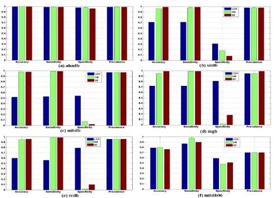
The classification performance is shown in Fig.10, which compares the performance of classification methods LDA, NB and RF, based on datasets (a)ahadb, (b)sddb, (c)
[image:16.612.188.430.92.235.2] [image:16.612.169.454.288.424.2]Fig. 10. Classification performance of six datasets based on the summarized features using classification methods of LDA, RF, and NB
Fig. 11. Performance of seven classifiers (LDA, NB, DT, Ada, LPB, Ttl, and RUS) based on the proposed period identification and segmentation methods on five datasets ((a) ahadb, (b) ltdb, (c) mitdb, (d) sddb, and (e) svdb)
5.4. Performance Evaluation of Other Classification Methods Based on Summarized Features
[image:17.612.114.504.332.504.2]methods: AdaBoost (Ada), LPBoost (LPB), TotalBoost (Ttl), and RUSBoost (RUS). The classification performance is validated by five benchmarks:acc,sen,f mea, andprev.
Fig.11 shows the evaluated results of the classifier performance based on the pro-posed period identification and segmentation method. From Fig.11, we can see that the accuracy values of classification based on the5 datasets are over90%, except the cases of LPB with mitdb, LDA withsddb, LDA with svdb, and RUS with svdb. Some of them are of more than 98%accuracy. The sensitivity of classification based on the datasets of ahadb, ltdb, and mitdb are closing to 100%. The sensitivity based on the datasets ofsddbandsvdbare over85%. The f-measure rates of classification based on
ahadb,ltdb,mitdb, andsddbare higher than95%. The f-measure rates of RUS and LDA
based onmitdbandsvdbare less than80%, but the f-measure of other classifiers based on these two datasets are all higher than80%, and some of them are closing to100%. The prevalence rates of classification on the basis of the five datasets are over90%.
6. CONCLUSIONS
In this paper, we have introduced a framework of detecting anomalies in uncertain pseudo periodic time series. We formally define pseudo periodic time series (P T S) and identified three types of anomalies that may occur in aP T S. We focused on local anomaly detection inP T Sby using classification tools. The uncertainties in aP T Sare pre-processed by an inflexion detecting procedure. By conducting DP-based time se-ries compression and feature summarization of each segment, the proposed approach significantly improves the time efficiency of time series processing and reduces the storage space of the data streams. One problem of the proposed framework is that the silhouette coefficient based clustering evaluation is a time consuming process. Though the compressed time series contains much fewer data points than the raw time se-ries, it is necessary to develop a more efficient evaluation approach to find the optimal clusters of data stream inflexions. In the future, we are going to find a more time ef-ficient way to recognize the patterns of a P T S. In addition, we will do more testing based on other datasets to further validate the performance of the method. Correcting false-detected inflexions and detecting global anomalies in an uncertain P T S will be the main target of our next research work.
Acknowledgement
This work is supported by the National Natural Science Foundation of China (NSFC 61332013) and the Australian Research Council (ARC) Discovery Projects DP140100841, DP130101327, and Linkage Project LP100200682.
REFERENCES
Charu C. Aggarwal. 2009. On high dimensional projected clustering of uncertain data streams. In IEEE 25th International Conference on Data Engineering (ICDE’09). IEEE, Shanghai, China, 1152–1154. DOI:http://dx.doi.org/10.1109/ICDE.2009.188
Charu C. Aggarwal and Philip S. Yu. 2008. A framework for clustering uncertain data streams. In IEEE 24th International Conference on Data Engineering (ICDE’08). IEEE, Cancun, Mexico, 150–159. DOI:http://dx.doi.org/10.1109/ICDE.2008.4497423
Ian F. Akyildiz, Dario Pompili, and Tommaso Melodia. 2005. Underwater acoustic sensor networks: research challenges. Ad Hoc Netw. 3, 3 (2005), 257–279.DOI:http://dx.doi.org/10.1016/j.adhoc.2005.01.004 Lv an Tang, Bin Cui, Hongyan Li, Gaoshan Miao, Dongqing Yang, and Xinbiao Zhou. 2007. Effective
variation management for pseudo periodical streams. In Proceedings of the 2007 ACM SIGMOD International Conference on Management of Data (SIGMOD’07). ACM, New York, NY, USA, 257–268. DOI:http://dx.doi.org/10.1145/1247480.1247511
David Arthur and Sergei Vassilvitskii. 2007. K-means++: the advantages of careful seeding. In Proceedings of the Eighteenth Annual ACM-SIAM Symposium on Discrete Algorithms (SODA’07). Society for In-dustrial and Applied Mathematics, Philadelphia, PA, USA, 1027–1035. http://dl.acm.org/citation.cfm? id=1283383.1283494
Johannes Aßfalg, Hans-Peter Kriegel, Peer Kr¨oger, and Matthias Renz. 2009. Probabilistic similarity search for uncertain time series. In Scientific and Statistical Database Management, Marianne Winslett (Ed.). Lecture Notes in Computer Science, Vol. 5566. Springer Berlin Heidelberg, New Orleans, LA, USA, 435–443.DOI:http://dx.doi.org/10.1007/978-3-642-02279-1 31
Jianjun Chen, David J. DeWitt, Feng Tian, and Yuan Wang. 2000. NiagaraCQ: a scalable continuous query system for internet databases. In Proceedings of ACM SIGMOD International Conference on Management of Data (SIGMOD’00). 379–390. http://doi.acm.org/10.1145/342009.335432
CSIRO. 2011. Sensors and Sensor Networks 2010-2011 Year in Review. (2011). http://research.ict.csiro.au/ news/sensors-and-sensor-networks-2010-2011-year-in-review
Michele Dallachiesa, Besmira Nushi, Katsiaryna Mirylenka, and Themis Palpanas. 2012. Uncertain time-series similarity: return to the basics. Proc. VLDB Endow. 5, 11 (July 2012), 1662–1673. DOI:http://dx.doi.org/10.14778/2350229.2350278
David H. Douglas and Thomas K. Peucker. 1973. Algorithms for the reduction of the number of points required to represent a digitized line or its caricature. Cartographica 10, 2 (1973), 112–122.
Philippe Esling and Carlos Agon. 2012. Time-series data mining. ACM Comput. Surv. 45, 1, Article 12 (December 2012), 12:1–12:34 pages.DOI:http://dx.doi.org/10.1145/2379776.2379788
Victor A. Folarin, Patrick J. Fitzsimmons, and William B. Kruyer. 2001. Holter monitor findings in asymp-tomatic male military aviators without structural heart disease. Aviat. Space. Envir. MD 72, 9 (2001), 836–838. http://www.ncbi.nlm.nih.gov/pubmed/11565820
Ary L. Goldberger, Luis AN Amaral, Leon Glass, Jeffrey M. Hausdorff, Plamen Ch Ivanov, Roger G. Mark, Joseph E. Mietus, George B. Moody, Chung-Kang Peng, and H. Eugene Stanley. 2000a. Physiobank, physiotoolkit, and physionet: components of a new research resource for complex physiologic signals. Circulation 101, 23 (2000), e215–e220.
Ary L. Goldberger, Luis AN Amaral, Leon Glass, Jeffrey M. Hausdorff, Plamen Ch Ivanov, Roger G. Mark, Joseph E. Mietus, George B. Moody, Chung-Kang Peng, and H. Eugene Stanley. 2000b. PhysioBank, PhysioToolkit, and PhysioNet: Components of a New Research Resource for Complex Physiologic Sig-nals. Circulation 101, 23 (2000).DOI:http://dx.doi.org/10.1161/01.CIR.101.23.e215
Aslak Grinsted, John C. Moore, and Svetlana Jevrejeva. 2004. Application of the cross wavelet transform and wavelet coherence to geophysical time series. Nonlinear Proc. Geoph. 11, 5/6 (2004), 561–566. DOI:http://dx.doi.org/10.5194/npg-11-561-2004
Yu Gu, Andrew McCallum, and Don Towsley. 2005. Detecting anomalies in network traffic using maximum entropy estimation. In Proceedings of the 5th ACM SIGCOMM Conference on Internet Measurement (IMC’05). USENIX Association, Berkeley, CA, USA, 32–32. http://dl.acm.org/citation.cfm?id=1251086. 1251118
Joachim Gudmundsson, Marc van Kreveld, and Bettina Speckmann. 2007. Efficient detection of patterns in 2D trajectories of moving points. GeoInformatica 11, 2 (2007), 195–215. DOI:http://dx.doi.org/10.1007/s10707-006-0002-z
S¸ ule G ¨und ¨uz and M Tamer ¨Ozsu. 2003. A web page prediction model based on click-stream tree representa-tion of user behavior. In Proceedings of the 9th ACM SIGKDD Internarepresenta-tional Conference on Knowledge Discovery and Data Mining. ACM, 535–540.
John A. Hartigan and Manchek A. Wong. 1979. Algorithm AS 136: a K-means clustering algorithm. J. Roy. Stat. Soc. C.-APP 28, 1 (1979), 100–108. http://www.jstor.org/stable/2346830
Jing He, Yanchun Zhang, and Guangyan Huang. 2012. Exceptional object analysis for finding rare environmental events from water quality datasets. Neurocomputing 92, 0 (2012), 69–77. DOI:http://dx.doi.org/10.1016/j.neucom.2011.08.036 Data Mining Applications and Case Study. Jing He, Yanchun Zhang, Guangyan Huang, and Paulo de Souza. 2013. CIRCE: correcting imprecise
read-ings and compressing excrescent points for querying common patterns in uncertain sensor streams. Inform. Syst. 38, 8 (2013), 1234–1251.DOI:http://dx.doi.org/10.1016/j.is.2012.01.003
John Hershberger and Jack Snoeyink. 1994. An O(Nlogn) implementation of the Douglas-Peucker algo-rithm for line simplification. In Proceedings of the 10th Annual Symposium on Computational Geometry (SCG’94). ACM, New York, NY, USA, 383–384.DOI:http://dx.doi.org/10.1145/177424.178097
Ruoyi Jiang, Hongliang Fei, and Jun Huan. 2011. Anomaly localization for network data streams with graph joint sparse PCA. In Proceedings of the 17th ACM SIGKDD International Conference on Knowledge Discovery and Data Mining (KDD’11). ACM, New York, NY, USA, 886–894. DOI:http://dx.doi.org/10.1145/2020408.2020557
Eamonn Keogh, Jessica Lin, and Ada Fu. 2005. HOT SAX: efficiently finding the most unusual time series subsequence. In The 5th IEEE International Conference on Data Mining (ICDM’05). IEEE, Houston, Texas, USA, 226–233.DOI:http://dx.doi.org/10.1109/ICDM.2005.79
Eamonn J. Keogh, Selina Chu, David Hart, and Michael Pazzani. 2004. Segmenting time series: a survey and novel approach. In Data Mining In Time Series Databases, Mark Last, Abraham Kandel, and Horst Bunke (Eds.). Series in Machine Perception and Artificial Intelligence, Vol. 57. World Scientific Publishing Company, Chapter 1, 1–22.
Jae-Gil Lee, Jiawei Han, and Kyu-Young Whang. 2007. Trajectory clustering: a partition-and-group frame-work. In Proceedings of the 2007 ACM SIGMOD International Conference on Management of Data (SIGMOD’07). ACM, New York, NY, USA, 593–604.DOI:http://dx.doi.org/10.1145/1247480.1247546 Daniel Lemire. 2007. A better alternative to piecewise linear time series segmentation. In Proceedings of
the 7th SIAM International Conference on Data Mining (April 26-28) (SDM’07). 545–550.
Carson Kai-Sang Leung and Boyu Hao. 2009. Mining of frequent item-sets from streams of uncertain data. In IEEE 25th International Conference on Data Engineering (ICDE’09). IEEE, Shanghai, China, 1663– 1670.DOI:http://dx.doi.org/10.1109/ICDE.2009.157
Matthew N. Levy and Achilles J. Pappano. 2007. Cardiovascular physiology. Mosby Elsevier.
Bai ling Zhang, Yanchun Zhang, and Rezaul K. Begg. 2009. Gait classification in chil-dren with cerebral palsy by Bayesian approach. Pattern Recogn. 42, 4 (2009), 581–586. DOI:http://dx.doi.org/10.1016/j.patcog.2008.09.025 Pattern Recognition in Computational Life Sci-ences.
Xiaoyan Liu, Xindong Wu, Huaiqing Wang, Rui Zhang, J. Bailey, and K. Ramamohanarao. 2010. Mining distribution change in stock order streams. In IEEE 26th International Conference on Data Engineering (VLDB’04). 105–108.DOI:http://dx.doi.org/10.1109/ICDE.2010.5447901
Melanie Manning and Louanne Hudgins. 2010. Array-based technology and recommendations for utilization in medical genetics practice for detection of chromosomal abnormalities. Genet. Med. 12, 11 (2010), 742– 745.
Andrew Y. Ng, Michael I. Jordan, Yair Weiss, and others. 2001. On spectral clustering: analysis and an algorithm. In Advances in Neural Information Processing Systems, T.G. Dietterich, S. Becker, and Z. Ghahramani (Eds.). Vol. 14. MIT Press, Cambridge, USA, 849–856.
Themis Palpanas, Michail Vlachos, Eamonn Keogh, and Dimitrios Gunopulos. 2008. Streaming time series summarization using user-defined amnesic functions. IEEE Trans. Knowl. Data Eng. 20, 7 (July 2008), 992–1006.DOI:http://dx.doi.org/10.1109/TKDE.2007.190737
Jianzhong Qi, Rui Zhang, Kotagiri Ramamohanarao, Hongzhi Wang, Zeyi Wen, and Dan Wu. 2015. In-dexable online time series segmentation with error bound guarantee. World Wide Web 18, 2 (2015), 359–401.DOI:http://dx.doi.org/10.1007/s11280-013-0256-y
Douglas Reynolds. 2009. Gaussian Mixture Models. In Encyclopedia of Biometrics, StanZ. Li and Anil Jain (Eds.). Springer, USA, 659–663.DOI:http://dx.doi.org/10.1007/978-0-387-73003-5 196
Paul L. Rosin. 2003. Assessing the behaviour of polygonal approximation algorithms. Pattern Recogn. 36, 2 (2003), 505–518.DOI:http://dx.doi.org/10.1016/S0031-3203(02)00076-6 Biometrics.
Peter J. Rousseeuw. 1987. Silhouettes: a graphical aid to the interpretation and validation of cluster analy-sis. J. Comput. Appl. Math. 20, 0 (1987), 53–65.DOI:http://dx.doi.org/10.1016/0377-0427(87)90125-7 Smruti R. Sarangi and Karin Murthy. 2010. DUST: a generalized notion of similarity between
uncertain time series. In Proceedings of the 16th ACM SIGKDD International Conference on Knowledge Discovery and Data Mining (KDD’10). ACM, New York, NY, USA, 383–392. DOI:http://dx.doi.org/10.1145/1835804.1835854
Galit Shmueli and Howard Burkom. 2010. Statistical challenges facing early outbreak detection in bio-surveillance. Technometrics 52, 1 (2010), 39–51.
Ikaro Silva and George Moody. 2014. An Open-source Toolbox for Analysing and Processing PhysioNet Databases in MATLAB and Octave. J. Open Res. Softw. 2, 1 (2014).
Mahbod Tavallaee, Natalia Stakhanova, and Ali Akbar Ghorbani. 2010. Toward credible evaluation of anomaly-based intrusion-detection methods. IEEE T. Syst. Man. Cy. C. 40, 5 (September 2010), 516– 524.DOI:http://dx.doi.org/10.1109/TSMCC.2010.2048428
William Wilson, Phil Birkin, and Uwe Aickelin. 2008. The motif tracking algorithm. International Journal of Automation and Computing 5, 1 (2008), 32–44.
Zhenghua Xu, Rui Zhang, Ramamohanarao Kotagiri, and Udaya Parampalli. 2012. An adaptive algo-rithm for online time series segmentation with error bound guarantee. In Proceedings of the 15th International Conference on Extending Database Technology (EDBT’12). ACM, New York, NY, USA, 192–203.DOI:http://dx.doi.org/10.1145/2247596.2247620
Yu Zheng, Xing Xie, and Wei-Ying Ma. 2010. GeoLife: a collaborative social networking service among user, location and trajectory. IEEE Data Eng. Bull. 33, 2 (2010), 32–39. http://sites.computer.org/debull/ A10june/geolife.pdf