Type theory in type theory using quotient inductive types

Co nsist

ent *Complete*

W

ellD_o

cu

m

en

ted

*E asy

to

Re

us

e

* *

Ev

alu

ate d * PO

P

L*

Artifact *

A

EC

Type Theory in Type Theory using Quotient Inductive Types

∗

Thorsten Altenkirch

Ambrus Kaposi

School for Computer Science, University of Nottingham, United Kingdom

{txa,auk}@cs.nott.ac.uk

Abstract

We present an internal formalisation of a type heory with dependent types in Type Theory using a special case of higher inductive types from Homotopy Type Theory which we call quotient inductive types (QITs). Our formalisation of type theory avoids referring to preterms or a typability relation but defines directly well typed objects by an inductive definition. We use the elimination principle to define the set-theoretic and logical predicate interpretation. The work has been formalized using the Agda system extended with QITs using postulates.

Categories and Subject Descriptors D.3.1 [Formal Definitions and Theory]; F.4.1 [Mathematical Logic]: Lambda calculus and related systems

Keywords Higher Inductive Types, Homotopy Type Theory, Log-ical Relations, Metaprogramming, Agda

1.

Introduction

We would like to reflect the syntax and typing rules of Type The-ory in itself. This offers exciting opportunities for typed metapro-gramming to support interactive theorem proving. We can also im-plement extensions of Type Theory by providing a sound interpre-tation giving rise to a form of template Type Theory. This paper describes a novel approach to achieve this ambition.

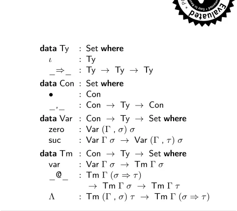
Within Type Theory it is straightforward to represent the simply

typedλ-calculus as an inductive type where contexts and types are

defined as inductive types and terms are given as an inductively defined family indexed by contexts and types (see figure 1 for a definition in idealized Agda).

Here we inductively define Types (Ty) and contexts (Con) which in a de Bruijn setting are just sequences of types. We define

the families of variables and terms where variables aretyped de

Bruijn indicesand terms are inductively generated from variables

using application (_@_) and abstraction (Λ).1

In this approach we never define preterms and a typing rela-tion but directly present the typed syntax. This has technical

advan-∗_{Supported by EPSRC grant EP/M016951/1.}

1_{We are oversimplifying things a bit here: we would really like to restrict}

operations to those which preserveβη-equality, i.e. work with a quotient of

Tm.

dataTy : Setwhere

ι : Ty

_⇒_ : Ty → Ty → Ty

dataCon : Setwhere

• : Con

_,_ : Con → Ty → Con

dataVar : Con → Ty → Setwhere

zero : Var(Γ,σ)σ

suc : VarΓσ → Var(Γ,τ)σ

dataTm : Con → Ty → Setwhere

var : VarΓσ → TmΓσ

_@_ : TmΓ (σ⇒τ)

→ TmΓσ → TmΓτ

Λ : Tm(Γ,σ)τ → TmΓ (σ⇒τ)

Figure 1. Simply typedλ-calculus

tages: in typed metaprogramming we only want to deal with typed syntax and it avoids the need to prove subject reduction theorems separately. But more importantly this approach reflects our type-theoretic philosophy that typed objects are first and preterms are designed at a 2nd step with the intention that they should contain enough information so that we can reconstruct the typed objects. Typechecking can be expressed in this view as constructing a par-tial inverse to the forgetful function which maps typed into untyped syntax (a sort of printing operation).

Naturally, we would like to do the same for the language we are working in, that is we would like to perform typed metapro-gramming for a dependently typed language. There are at least two complications:

(1) types, terms and contexts have to be defined mutually but also depend on each other,

(2) due to the conversion rule which allows us to coerce terms along type-equality we have to define the equality mutually with the syntactic typing rules:

Γ`A = B Γ`t : A

Γ`t : B

(1) can be addressed by using inductive-inductive definitions [6] (see section 2.1) – indeed doing Type Theory in Type Theory was one of the main motivations behind introducing inductive-inductive types. It seemed that this would also suffice to address (2), since we can define the conversion relation mutually with the rest of the syntax. However, it turns out that the overhead in form of type-theoretic boilerplate is considerable. For example terms depend on both contexts and types, we have to include special constructors which formalize the idea that this is a setoid indexed over two

This is the author’s version of the work. It is posted here for your personal use. Not for redistribution. The definitive version was published in the following publication:

POPL’16, January 20–22, 2016, St. Petersburg, FL, USA ACM. 978-1-4503-3549-2/16/01...

given setoids. Moreover each constructor comes with a congruence rule. In the end the resulting definition becomes unfeasible, almost impossible to write down explicitly but even harder to work with in practice.

This is where Higher Inductive Types [31] come in, because they allow us to define constructors for equalities at the same time as we define elements. Hence we can present the conversion relation just by stating the equality rules as equality constructors. Since we are defining equalities we don’t have to formalize any indexed setoid structure or explicitly state congruence rules. This second step turns out to be essential to have a workable internal definition of Type Theory.

Indeed, we only use a rather simple special case of higher in-ductive types, namely we are only interested in first order equal-ities and we are ignoring higher equalequal-ities. This is what we call Quotient Inductive Types (QITs). From the perspective of Homo-topy Type Theory QITs are HITs which are truncated to be sets. The main aspect of HITs we are using is that they allow us to in-troduce new equalities and constructors at the same time. This has already been exploited in a different way in [31] for the definition of the reals and the constructible hierarchy without having to use the axiom of choice.

1.1 Overview of the Paper

We start by explaining in some detail the type theory we are using as a metatheory and how we implement it using Agda in section 2. In particular we are reviewing inductive-inductive types (section 2.1) and we motivate the importance of QITs as simple HITs (section 2.2). Then, in section 3 we turn to our main goal and

define the syntax of a basic type theory with onlyΠ-types and an

uninterpreted universe with explicit substitutions. We explain how a general recursor and eliminator can be derived. As a warm-up we

define formally thestandard interpretationwhich interprets every

piece of syntax by the corresponding metatheoretic construction in section 4. Our main real-world example (section 5) is to formally give the logical predicate translation which has been introduced by Bernardy [7] to explain parametricity for dependent types. The constructions presented in this paper have been formalized in Agda, this is available as supplementary material [3].

1.2 Related Work

Our goal is to give a faithful exposition of the typed syntax of Type Theory in a first order setting in the sense that our syntax is finitary. Hence what we are doing is different from e.g. [10] which defines a higher order syntax for reflection. We also diverge from [24] which exploits the metatheoretic equality to make reflection feasible because we would like to have the freedom to interpret equality in any way we would like. We also note the work [14] which provides a very good motivation for our work but treats definitional equality in a non-standard way. Indeed, we want to express the syntax of Type Theory in a natural way without any special assumptions.

The work by Chapman [12] and also the earlier work by Danielsson [13] have a motivation very similar to ours. [13] uses implicit substitutions and this seems rather difficult to use in gen-eral, his definitions have rather adhoc character. [12] is more prin-cipled but relies on setoids and has to add a lot of boilerplate code to characterize families of setoids over a setoid explicitly. This boilerplate makes the definition in the end unusable in practice.

A nice application of type-theoretic metaprogramming is de-veloped in [20] where the authors present a mechanism to safely extend Coq with new principles. This relies on presenting a proof-irrelevant presheaf model and then proving constants in the presheaf interpretation. Our approach is in some sense complemen-tary in that we provide a safe translation from well typed syntax

into a model, but also more general because we are not limited to any particular class of models.

Our definition of the internal syntax of Type Theory is very much inspired by categories with families (CwFs) [16, 19]. Indeed, one can summarize our work by saying that we construct an initial CwF using QITs. That something like this should be possible in principle was clear since a while, however, the progress reported here is that we have actually done it.

The style of the presentation can also be described as a gener-alized algebraic theory [11] which has been recently used by Co-quand to give very concise presentations of Type Theory [8]. Our work shows that it should be possible to internalize this style of presentation in type theory itself.

Higher Inductive Types are described in chapter 6 in [31], and it is shown that they generalize quotient types, e.g. see [18, 25].

2.

The Type Theory We Live In

We are working in a Martin-Löf Type Theory using Agda as a ve-hicle. That is our syntax is the one used by the functional program-ming language and interactive proof assistant Agda [2, 27]. In the paper, to improve readability we omit implicitly quantified vari-ables whose types can be inferred from the context (in this respect we follow rather Idris [9]).

In Agda,Π-types are written as(x:A) → BforΠ(x:A).B,

implicit arguments are indicated by curly brackets{x:A} → B,

these can be omitted if Agda can infer them from the types of later arguments. Agda supports mixfix notation, eg. function space can

be denoted_⇒_where the underscores show the placement of

ar-guments. Underscores can also be used when defining a function if we are not interested in the value of the argument eg. the constant

function can be defined asconst x = x. The keyworddata

is used to define inductively generated families and the keyword

recordis for defining dependent record types (iteratedΣ-types) by

listing their fields after the keywordfield. Records are

automati-cally modules (separate name spaces) in Agda, this is why they can

be opened using theopenkeyword. In this case the field names

be-come projection functions. Just as inductive types can have parame-ters, records and modules can also be parameterised (by a telescope of types), we use this feature of Agda to structure our code. Agda allows overloading of constructor names, we use this e.g. when

us-ing the same constructor_,_for context extension and

substitu-tion extension. Equality (or the identity type) is denoted by_≡_

and has the constructorrefl. We use the syntaxa≡[ p ]≡bto

ex-press that two objects in different typesa:Aandb:Bare equal via

an equality of their typesp : A ≡ B, see also section 3.

To support this flexible syntax Agda diverges from most

pro-gramming languages in that space matters. E.g._JΓ_Kis just a

vari-able name but_JΓ_Kis the application of the operation_J__KtoΓ.

We use QITs which are not available in Agda, however we can simulate them by a technique pioneered by [22] for HITs. While QITs are a special case of HITs and are inspired by Homotopy Type Theory (HoTT), for most of the paper we shall work with a type theory with a strict equality, i.e. we assume that all equality proofs are equal. We will get back to this issue and explain how our work relates to Homotopy Type Theory in section 6.

However, we do assume functional extensionality which follows in any case from the presence of QITs. The theory poses a

canon-icity problem, i.e. can all closed term of typeNbe reduced to

nu-merals, which can be adressed using techniques developed in the

context ofObservational Type Theory[5]. Recent work [8]

2.1 Inductive-Inductive Types

One central construction in Type Theory areinductive types, where

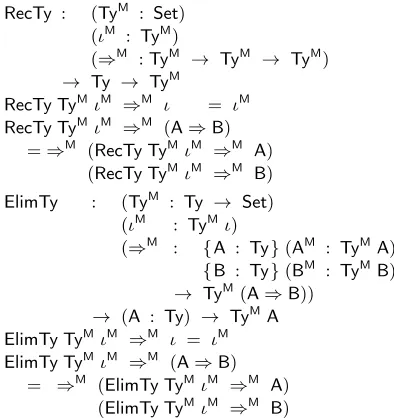
types are specified using constructors - see the definition of types and contexts in figure 1. In practical dependently typed program-ming we use pattern matching - however it is good to know that this can be replaced by adding just one elimination constant to each inductive type we are defining [23]. Here we differentiate between therecursorwhich enables us to define non-dependent functions and the eliminator which allows the definition of dependent func-tions. The latter corresponds logically to an induction principle for the given type. Note that the recursor is just a special case of the eliminator. As an example consider the recursor and the eliminator

for the inductive typeTydefined in figure 1:

RecTy : (TyM : Set)

(ιM : TyM) (⇒M

:TyM → TyM → TyM)

→ Ty → TyM

RecTyTyM_ιM _⇒M _{ι = ι}M

RecTyTyMιM ⇒M

(A⇒B) =⇒M

(RecTyTyMιM ⇒M _A

)

(RecTyTyMιM ⇒M

B)

ElimTy : (TyM _{: Ty → Set)}

(ιM : TyMι) (⇒M

: {A : Ty}(AM : TyMA) {B : Ty}(BM : TyMB) → TyM(A⇒B))

→ (A : Ty) → TyM_A

ElimTyTyM_ιM _⇒M _{ι = ι}M

ElimTyTyMιM ⇒M

(A⇒B)

= ⇒M

(ElimTyTyMιM ⇒M _A

)

(ElimTyTyMιM ⇒M _B

)

The type/dependent type we use in the recursor/eliminator (TyM

)

we call themotiveand the functions corresponding to the

construc-tors (ιM,⇒M

) are themethods. The motive and the methods of the

recursor are thealgebrasof the corresponding signature functor.

The motiveTyM

is afamily indexedoverTyand the methods are

fibersof the family over the constructors.

We can also define dependent families of types inductively

-examples areVarandTmin figure 1. We may extend this to mutual

inductive types or mutual inductive dependent types — however they can be reduced to a single inductive family by using an extra

parameter of typeBoolwhich provides the information which type

is meant.

However, there are examples of mutual definitions which are not covered by this explanation: that is if we define a type and a family which depends on this type mutually. In this case we may also refer to constructors which have been defined previously. A canonical example for this is a fragment of the definition of the syntax of dependent types where we only define types and contexts (figure 2). Indeed we have to define types and contexts at the same time but types are indexed by contexts to express that we want to define the type of valid types in a given context. The constructor

_,_appears in the type of theΠ-constructor to express that the

codomain type lives in the context extended by the domain type.

The definition of suchinductive-inductivetypes in Agda is

stan-dard. We first declare the types of all the types we want to define inductively but without giving the constructors and then complete the definition of the constructors when all the type signatures are in scope.

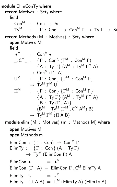
As before, programming with inductive-inductive types can be reduced to using the elimination constants - see figures 3 and 4 for

dataCon : Set

dataTy : Con → Set

dataConwhere

• : Con

_,_ : (Γ : Con) → TyΓ → Con

dataTywhere

U : ∀ {Γ} → TyΓ

Π : ∀ {Γ}(A : TyΓ) (B : Ty(Γ, A)) → TyΓ

Figure 2. An example of an inductive-inductive type: contexts and types in a dependent type theory

moduleRecConTywhere recordMotives : Set1 where

field

ConM : Set

TyM : ConM → Set

recordMethods(M : Motives) : Set1where

openMotives M

field

•M _{: Con}M

_,CM_{_ : (Γ}M _{: Con}M_{) → Ty}M_ΓM _{→ Con}M

UM _{: {Γ}M _{: Con}M_{} → Ty}M_ΓM

ΠM _{: {Γ}M _{: Con}M_}(AM _{: Ty}M_ΓM₎

(BM : TyM(ΓM,CMAM)) → TyMΓM modulerec(M : Motives) (m : Methods M)where

openMotives M

openMethods m

RecCon : Con → ConM

RecTy : {Γ : Con}(A : TyΓ) → TyM(RecConΓ)

RecCon• = •M

RecCon(Γ, A) = RecConΓ,CMRecTy A

RecTy U = UM

RecTy (ΠA B) = ΠM_{(RecTy A) (RecTy B)}

Figure 3. Recursor for the inductive-inductive type of figure 2

those of the mutual inductive typesConandTydefined in figure

2. To make working with complex elimination constants feasible

we organize their parameters into records:Motives,Methods. The

motives and methods for the recursor can be defined just by adding

M

indices to the types of the types and constructors. Defining the motives and methods for the eliminator is more subtle: we need to define families over the types and fibers of those families over the constructors taking into account the mutual dependencies — see

section 5.3 for a generic way of deriving these. Theβ-rules can

be added to the system by pattern matching on the constructors — these rules are the same for the recursor and the eliminator.

moduleElimConTywhere recordMotives : Set1where

field

ConM _{: Con → Set}

TyM _{: {Γ : Con} → Con}M_{Γ → TyΓ → Set}

recordMethods(M : Motives) : Set1where

openMotives M

field •M

: ConM•

_,CM_ : {Γ : Con}(ΓM : ConMΓ)

{A : TyΓ}(AM : TyMΓMA) → ConM(Γ, A)

UM _{: {Γ : Con} {Γ}M _{: Con}M_Γ}

→ TyM_ΓM_U

ΠM _{: {Γ : Con} {Γ}M _{: Con}M_Γ}

{A : TyΓ}(AM _{: Ty}M_ΓM_A)

{B : Ty(Γ, A)}

(BM : TyM(ΓM,CMAM)B) → TyM_ΓM_{(ΠA B)}

moduleelim(M : Motives) (m : Methods M)where

openMotives M

openMethods m

ElimCon : (Γ : Con) → ConM_Γ

ElimTy : {Γ : Con}(A : TyΓ)

→ TyM(ElimConΓ)A

ElimCon • = •M

ElimCon (Γ, A) = ElimConΓ,CMElimTy A

ElimTy U = UM

ElimTy (ΠA B) = ΠM(ElimTy A) (ElimTy B)

Figure 4. Eliminator for the inductive-inductive type of figure 2

2.2 Quotient Inductive Types (QITs)

One of the main applications of Higher Inductive Types in Homo-topy Type Theory is to represent types with non-trivial equalities corresponding to the path spaces of topological spaces. Here we are working in a Type Theory with a strict equality, i.e. all higher path spaces are trivial. However, there are still interesting applica-tions for these degenerate HITs which we call Quotient Inductive Types (QITs). E.g. in [31] QITs (even though not by that name) are used to define the constructible hierarchy of sets in an encoding of set theory within HoTT and later to define the Cauchy Reals. What is striking is that in both cases ordinary quotient types would not have been sufficient but would have required some form of the axiom of choice.

Agda does not allow the definition of equality constructors for inductive types, however following [22] we can simulate them by postulating the equality constructors and defining the recur-sor/eliminator by pattern matching (see eg. figures 5 and 6). This is the only place where we are allowed to pattern match on an element of a QIT: later we should only use the eliminator/recursor. This can be enforced by hiding techniques or turning off pattern match-ing. Using this technique we retain the computational behaviour of lower constructors while enforcing respect for the higher construc-tors. The computation rules for the equality constructors always hold (propositionally) because we work in a theory with UIP. We conjecture that the logical consistency of Agda extended by QITs

data_/_(A : Set) (R : A → A → Set) : Setwhere

[_] : A → A / R

postulate

[_]≡ : ∀ {A} {R : A → A → Set} {a b : A}

→ R a b → [a] ≡ [b]

moduleElim_/_

(A : Set) (R : A → A → Set) (QM _{: A / R → Set)}

([_]M _{: (a : A) → Q}M_[a])

([_]≡M _{: {a b : A}(r : R a b)}

→ [a]M_{≡[ apQ}M_{[r ]≡]≡[b]}M₎

where

Elim : (x : A / R) → QMx

Elim[x ] = [x]M

Figure 5. The constructors and elimination principle for quotient

types in HoTT-style. Note that the[_]≡equality constructor needs

to be postulated and pattern matching on elements ofA / Ris

disallowed except when definingElim(this is not checked by Agda,

we need to ensure this by hand): the only way to define a function

fromA / Rshould be using the eliminator.

can be justified by the setoid model. For the more general case of HITs, some examples have been studied in the context of cubical type theory [8].

While this is not the use of quotient inductive types which is directly relevant for our representation of dependently typed calculi it is worthwhile to explain this in some detail to make clear what QITs are about.

Our goal is to define infinitely branching trees where the actual order of subtrees doesn’t matter. We start by defining the type of infinite trees:

dataT0 : Setwhere

leaf : T0

node : (N → T0) → T0

and now we specify an equivalence relation which allows us to use an isomorphism to reorder a tree locally.

data_~_ : T0 → T0 → Setwhere

leaf : leaf∼leaf

node : {f g : _N → T0} → (∀ {n} → f n∼g n)

→ node f∼node g

perm : (g : N → T0) (f : N → N) → isIso f

→ node g∼node(g◦f)

HereisIso : (_N → N) → Setspecifies that the argument is an

isomorphism, i.e. there is an inverse function. Quotient types [18] can be postulated as shown in figure 5. With the help of this, we can construct the type:

T : Set

T = T0 / _~_

Note that this doesn’t require to show that_~_is an equivalence

relation but the resulting type is equivalent to the quotient with the

equivalence closure of the given relation. The elements ofT are

equivalence classes[ t ] : T0 / _~_and givenp : t ∼t’

we have[p ]≡ : [ t] ≡ [ t’]. The elimination principleElim

allows us to lift a function[_]Mwhich respects_~_(expressed by

[_]≡M_{) to any element of the quotient.}

We would expect that we should be able to liftnodeto

dataT : Setwhere

leaf : T

node : (_N → T) → T

postulate

perm : (g : N → T) (f : N → N) → isIso f

→ node g ≡ node(g◦f)

moduleElimT

(TM _{: T → Set)}

(leafM _{: T}M_leaf)

(nodeM _{: {f :}

N → T}(fM : (n : N) → TM(f n))

→ TM_{(node f))}

(permM : {g : N → T}(gM : (n : N) → TM(g n))

(f : N → N) (p : isIso f)

→ nodeM_gM_{≡[ apT}M_{(perm g f p)]≡}

nodeM_(gM_◦f))

where

Elim : (t : T) → TMt

Elim leaf = leafM

Elim(node f) = nodeM(λn → Elim(f n))

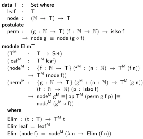
Figure 6. The constructors and eliminator for the

quotient-inductive typeT

T) → Tsuch that[node f] ≡ node’([_] ◦f). However, it

seems not possible to do this. To see what the problem is it is in-structive to solve the same exercise for finitely branching trees. It turns out that we have to sequentially iterate the eliminator depend-ing on the branchdepend-ing factor. However, clearly this approach doesn’t work for infinite trees. And indeed, in general assuming that we can lift function types of equivalence classes is equivalent to the axiom of choice. And this is an intuitionistic taboo since it entails the excluded middle [15].

However, if we use a QIT and specify the constructor for equal-ity at the same time we avoid this issue altogether. Such a version of

Tis defined in figure 6. The main difference here is that we specify

the new equality and the constructors at the same time. We also do not need to assume that the relation is a congruence because this is provable in general for the equality type. The dependent eliminator is given in figure 6: we see that we also need to interpret the

equa-tion when we eliminate fromT(pattern matching onTshould be

avoided after defining the eliminator).

Pitts [29] observed that an alternative way to solve this problem

would be to mutually define∼andT0and then useT = T0/_~

in the negative position of the constructors forT, i.e.

node : (N → T) → T0.

It seems plausible that QITs could be reduced to inductive-inductive definitions and quotient types and the reasonable assumption that quotient types preserves strict positivity.

3.

Representing the Syntax of Type Theory

We are now going to apply the tools introduced in the previous section to formalize a simple dependent type theory, that is a type

theory withΠ-types and an uninterpreted family denoted byU :

T ypeand El : U → T ype. Despite the naming this is not a

universe, but a base type in the same way asιis a base type for the

simply typedλcalculus. Without this the syntax would be trivial as

there would be no types or terms we could construct.

The signature of the QIT we are using to represent the syntax of

type theory is given in figure 7. We have already seen contextsCon

dataCon : Set

dataTy : Con → Set

dataTms : Con → Con → Set

dataTm : ∀Γ → TyΓ → Set

Figure 7. Signature of the syntax

dataConwhere

• : Con

_,_ : Con → Ty → Con

dataTywhere

_[_]T : Ty∆ → TmsΓ ∆ → TyΓ

Π : (A : TyΓ) (B : Ty(Γ, A)) → TyΓ

U : TyΓ

El : (A : TmΓU) → TyΓ

Figure 8. Constructors for contexts and types

dataTmswhere

: TmsΓ•

_,_ : (δ : TmsΓ ∆) → TmΓ (A[δ]T)

→ TmsΓ (∆, A)

id : TmsΓ Γ

◦ : Tms∆ Σ → TmsΓ ∆ → TmsΓ Σ

π1 : TmsΓ (∆, A) → TmsΓ ∆

Figure 9. Constructors for substitutions

and TypesTyin our previous example for an inductive-inductive

definition. We extend this by explicit substitutions (Tms) which

are indexed by two contexts and termsTmwhich are indexed by a

context and a type in the given context.

The constructors for contexts are exactly the same as in the pre-vious example but we are introducing some new constructors for types (figure 8). Most notably we introduce a substitution operator

_[_]Twhich applies a substitution fromΓto∆to a type in

con-text∆producing a type in contextΓ. The contravariant character

of substitution arises from the desire to semantically interpret sub-stitutions as functions going in the same direction, as we will see in detail in section 4. Syntactically it is good to think of an element of

TmsΓ ∆as a sequence of terms in contextΓwhich inhabit all the

types in∆. This intuition is reflected in the syntax for substitutions

(figure 9):is the empty sequence of terms, and_,_extends a

given sequence by an additional term. It is worthwhile to note that while the type which is added lives in the previous target context

∆, the term has free variables inΓwhich makes it necessary to

ap-ply the substitution operator on types:A[δ]T. We also introduce

inverses to_,_, i.e. projections. The first oneπ1 produces a

sub-stitution by forgetting the last term. Since we have explicit

substi-tutions we also have explicit composition ◦ of substitutions and

consequently also the identity substitution which will be essential when we reconstruct variables.

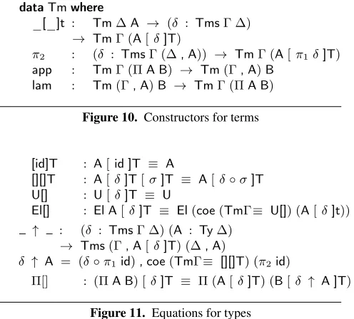
For terms (see figure 10) we also have a contravariant

substitu-tion operator_[_]twhose type uses the substitution operator for

types. We also introduce the second projectionπ2which projects

out the final term from a non-empty substitution. Finally, we

in-troduce app and lam which construct an isomorphism between

dataTmwhere

_[_]t : Tm∆A → (δ : TmsΓ ∆)

→ TmΓ (A[δ]T)

π2 : (δ : TmsΓ (∆, A)) → TmΓ (A[π1δ]T)

app : TmΓ (ΠA B) → Tm(Γ, A)B

lam : Tm(Γ, A)B → TmΓ (ΠA B)

Figure 10. Constructors for terms

[id]T : A[id ]T ≡ A

[][]T : A[δ]T[σ]T ≡ A[δ◦σ]T

U[] : U[δ]T ≡ U

El[] : El A[δ]T ≡ El(coe(TmΓ≡ U[]) (A[δ]t))

↑ : (δ : TmsΓ ∆) (A : Ty∆) → Tms(Γ, A[δ]T) (∆, A)

δ ↑ A = (δ◦π1id), coe(TmΓ≡ [][]T) (π2 id)

Π[] : (ΠA B) [δ]T ≡ Π (A[δ]T) (B[δ ↑ A ]T)

Figure 11. Equations for types

Let’s explore how our categorically inspired syntax can be used to derive more mundane syntactical components such as variables. First we derive the weakening substitution:

wk : ∀ {Γ} {A : TyΓ} → Tms(Γ, A) Γ

wk = π1id

We need to derive typed de Bruijn variables as in the example for

the simply typedλ-calculus. However, we have to be more precise

because the result types live in the extended context and hence we need weakening. However, the definitions are straightforward:

vz : Tm(Γ, A) (A[wk ]T)

vz = π2id

vs : TmΓA → Tm(Γ, B) (A[wk ]T)

vs x = x[wk ]t

Now we turn our attention to the constructors giving the

equa-tions. To define these we sometimes need totransport elements

along equalities. To simplify this we introduce a number of

conve-nient operations.coeturns an equality between types into a

func-tion:

coe : A ≡ B → A → B

Specifically in our current construction we often want to coerce terms along an equality of syntactic types, to facilitate this we introduce an operation which lifts an equality between syntactic types to an equality of semantic types of terms:

TmΓ≡ : {A0 : TyΓ} {A1 : TyΓ}(A2 : A0 ≡ A1)

→ TmΓA0 ≡ TmΓA1

A more general version of this function isap(apply path in HoTT

terminology):

ap : (f : A → B){a0a1 : A}(a2 : a0 ≡ a1)

→ f a0 ≡ f a1

We introduce no additional equations on contexts - however, the equality of contexts is not syntactic since they contain types which has non-trivial equalities.

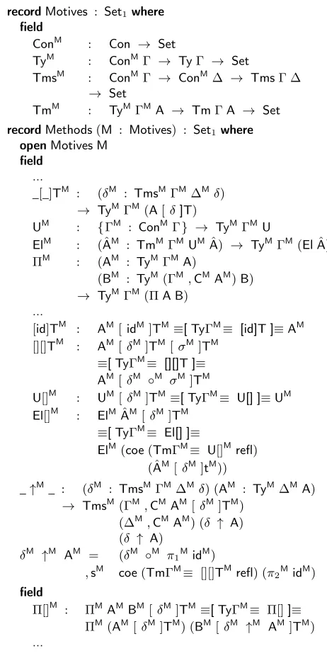
Let us turn our attention to syntactic typesTy, see figure 11.

The first two equations explain how substitution interacts with the identity substitution and composition. The remaining equations

idl : id◦δ ≡ δ

idr : δ◦id ≡ δ

ass : (σ◦δ)◦ν ≡ σ◦(δ◦ν)

,◦ : (δ, t)◦σ ≡ (δ◦σ), coe(TmΓ≡ [][]T) (t[σ]t)

π1β : π1(δ, t) ≡ δ

πη : (π1δ,π2δ) ≡ δ

η : {σ : TmsΓ•} → σ ≡

Figure 12. Equations for substitutions

[id]t : t[id ]t≡[TmΓ≡ [id]T ]≡t

[][]t : (t[δ]t) [σ]t≡[TmΓ≡ [][]T ]≡t[δ◦σ]t

π2β : π2(δ, a)≡[TmΓ≡ (ap(_[_]T A)π1β)]≡a

Πβ : app(lam t) ≡ t

Πη : lam(app t) ≡ t

lam[] : (lam t) [δ]t≡[TmΓ≡ Π[]]≡lam(t[δ ↑ A ]t)

Figure 13. Equations for terms

explain how substitutions move inside the other type constructors.

When introducing the equation forΠwe notice that we need to lift

a substitution along a type, that is given an element ofTmsΓ ∆we

want to deriveTms(Γ, A[δ]T) (∆, A). This is accomplished

by ↑ which can be defined using existing constructors of

substitutions and terms, namelyδ ↑ A = (δ ◦ wk , vz).

However this doesn’t typecheck since the second component of the

substitution should have typeTm(Γ, A[ δ]T) (A[ δ◦wk ]T)

butvzhas typeTm (Γ, A[δ ]T) (A[δ ]T [ wk ]T). However

using the equation just introduced which describes the interaction between substitution and composition can be used to fix this issue. The equations for substitutions (figure 12) state that

substitu-tions form a category and how composition commutes with_,_

which relies again on[][]T. We also state thatπ1works as expected

and that surjective pairing holds. There is only one substitution into

the empty context (η), this entails thatis a terminal object in the

category of substitutions.

The equations for terms (figure 13) start similarly to those for types: first we explain how term substitution interacts with the identity substitution and composition. Unsurprisingly, these laws

areupto the corresponding laws for types. We state the law for

the second projection whose typing relies on the equation for the

first projection. The equationsΠβandΠηstate thatlamandapp

are inverse to each other.lam[] explains how substitutions can

be moved intoλ-abstractions. This law refers to the substitution

law forΠ-types which can be viewed as an example of the

Beck-Chevalley condition [1]. Note that a corresponding law forappis

derivable:

app(coe(TmΓ≡ Π[]) (t[δ]t))

≡ hap(λz → app(coe(TmΓ≡ Π[]) (z[δ]t))) (Πη-1)i

app(coe(TmΓ≡ Π[]) ((lam(app t)) [ δ]t))

≡ hap app lam[]i

app(lam(app t[δ ↑ A ]t))

≡ hΠβi

app t[δ ↑ A ]t

We observe that our inductive definition defines an initial cate-gories with families (CwF) [16]. The equations can be summarized as follows: the contexts form a category with a terminal object and

we have the corresponding laws[id]T/t,[][]T/tfor substitutions

U[],El[],Π[]; the rest of the equations express two natural

isomor-phisms, one for the substitution extension_,_and one forΠ: the

βlaws express that going down and up is the identity, theηlaws

ex-press that going up and then down is the identity, while naturalities give the relationship with substitutions (an isomorphism is natural in both directions if it is natural in one direction).

_,_↓ ρ : TmsΓ ∆ TmΓ (A[ρ]T)

TmsΓ (∆, A) ↑π1,π2

lam↓ Tm(Γ, A)B

TmΓ (ΠA B) ↑app

We show how a more conventional application operator can be derived. First we introduce one term substitution:

<_> : TmΓA → TmsΓ (Γ, A)

< t > = id , coe(TmΓ≡ ([id]T-1

))t

Note that here we need to apply the equation for identity

substitu-tions backward exploiting symmetry for equasubstitu-tions_-1

. Given this it is easy to state and derive ordinary application:

$ : TmΓ (ΠA B) → (u : TmΓA)

→ TmΓ (B[< u > ]T)

t $ u = (app t) [< u > ]t

We prefer to use the categorical combinators in the definition of the syntax since they are easier to work with, avoiding unnecessary introduction of single term substitutions which correspond to using id.

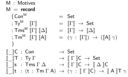
We define the recursor and the eliminator analogously to the examples in section 2. The motives and methods have the same

names as the types and constructors with an addedMindex. We list

the motives and the methods for types for the eliminator in figure

14. Note the usage of lifted congruence rules such asTyΓM≡and

TmΓM_{≡and how lifting the coerces is done. Also we define a}

lifting of the ↑ helper function.

An interpretation of the syntax can be given by providing

ele-ments of the recordsMotivesandMethods. Soundness is ensured

by the methods for equality constructors. This way a model of Type Theory can be viewed as an algebra of the syntax.

4.

The Standard Model

As a first sanity check of our syntax we define the standard model where every syntactic construct is interpreted by its semantic coun-terpart — this is also sometimes called the metacircular interpre-tation. That means we interpret contexts as types, types as depen-dent types indexed over the interpretation of their context, terms as dependent functions and substitutions as functions. We use the re-cursor to define this interpretation, the motives are given in figure 15. We use an idealized record notation where fields can have pa-rameters (in real Agda these need to be lambda expressions). The parameters of the fields of the motives are the results of the recur-sive calls of the recursor.

The definition of the methods is now straightforward (figure 16). In particular the interpretation of substitution nicely explains the

contravariant character of the substitution rules. Note thatJUK:Set

andJElK : JUK → Setare module parameters.

We have omitted the interpretation of all the equational

con-stants because they are trivial: all of them arereflbecause the two

sides are actually convertible in the metatheory.

A consequence of the standard model is soundness, that is in

our case we can show that there is no closed term ofUbecause we

can instantiateUwith the empty type. It should also be clear that to

construct the standard model we need a stronger metatheory than

recordMotives : Set1where field

ConM : Con → Set

TyM : ConMΓ → TyΓ → Set

TmsM : ConMΓ → ConM∆ → TmsΓ ∆

→ Set

TmM _{: Ty}M_ΓM_{A → TmΓA → Set}

recordMethods(M : Motives) : Set1where

openMotives M

field

...

_[_]TM : (δM : TmsMΓM∆Mδ)

→ TyMΓM(A[δ]T)

UM : {ΓM

: ConMΓ} → TyMΓMU

ElM : (ˆAM : TmMΓMUMAˆ) → TyMΓM(ElAˆ) ΠM : (AM : TyMΓMA)

(BM : TyM(ΓM,CMAM)B) → TyMΓM(ΠA B)

...

[id]TM : AM[idM]TM≡[TyΓM≡ [id]T ]≡AM

[][]TM : AM_[δM_]TM_[σM_]TM

≡[TyΓM≡ [][]T ]≡

AM[δM ◦M

σM]TM

U[]M : UM[δM]TM≡[TyΓM≡ U[] ]≡UM

El[]M : ElM_AˆM_[δM_]TM

≡[TyΓM_{≡ El[] ]≡}

ElM(coe(TmΓM≡ U[]Mrefl) (ˆAM[δM]tM))

_↑M

_ : (δM : TmsMΓM∆Mδ) (AM : TyM∆MA)

→ TmsM(ΓM,CMAM[δM]TM) (∆M,CMAM) (δ ↑ A) (δ ↑ A)

δM _↑M _AM _{= (δ}M _◦M _π

1MidM)

,sM coe(TmΓM≡ [][]TMrefl) (π2MidM)

field

Π[]M : ΠMAMBM[δM]TM≡[TyΓM≡ Π[]]≡ ΠM(AM[δM]TM) (BM[δM ↑M

AM]TM)

...

Figure 14. The motives and some methods for the eliminator for the syntax

the object theory we are considering. In our case this is given by the presence of an additional universe (here we have to eliminate

overSet1).

5.

The Logical Predicate Interpretation

auto-M : Motives M = record

{ConM = Set

;TyM _JΓ_K = _JΓ_K → Set

;TmsM_JΓ_{K J}∆_K = _JΓ_K → _J∆_K

;TmM _JΓ_{K J}A_K = (γ : _JΓ_K) → (_JA_Kγ) }

J_KC : Con → Set

J_KT : TyΓ → JΓKC → Set

J_Ks : TmsΓ ∆ → JΓKC → J∆KC

J_Kt : (t : TmΓA) → (γ : JΓKC) → JAKTγ

Figure 15. Motives for the standard model and how we would define the type of the interpretation functions using usual Agda syntax

m : Methods M

m = record { •M

= > ;_JΓ_K,CM_JA_K = Σ_JΓ_{K J}A_K

;_JA_K[_Jδ_K]TM_{γ =}

JAK(JδKγ)

;UM ₌

JUK

;ElM

JtK γ = JElK(JtKγ)

; ΠM

JAK JBK γ = (x : JAKγ) → JBK(γ, x)

;M _{= tt}

;_Jδ_K,sM_Jt_K γ = _Jδ_Kγ,_Jt_Kγ

;idM γ = γ

;_Jδ_K ◦M

JσK γ = JδK(JσKγ)

;π1M_Jδ_K γ = proj0(JδKγ)

;_Jt_K[_Jδ_K]tM γ = _Jt_K(_Jδ_Kγ) ;π2M_Jδ_K γ = proj1(JδKγ)

;appM_Jt_K γ = _Jt_K(proj0γ) (proj1γ)

;lamM

JtK γ = λa → JtK(γ, a)

; [id]TM = refl ...

}

Figure 16. Methods for the standard model

matically derive parametricity properties of functions defined in Agda.

5.1 Logical Relations for Dependent Types

Logical relations were introduced in computer science by Reynolds [30] for expressing the idea of representation-independence in the

context of the polymorphicλ-calculus. Reynold’s abstraction

theo-rem (also called parametricity) states that logically related interpre-tations of a term are logically related in the relation generated by the type of the term. This was later extended to dependent types by [7]: Type Theory is expressive enough to express the parametric-ity statement of its own terms — the logic in which the logical relations are expressed can be the theory itself. Contexts are inter-preted as syntactic contexts, types as types in the interpretation of their context and terms as witnesses of the interpretation of their types.

We describe the parametric interpretation for an explicit sub-stitution calculus with named variables, universes a la Russel, Pi

types and one universe. The syntax of contexts, terms and types is the following:

Γ ::= • | Γ, x : A

t,u,A,B ::= x | Set | (x:A) → B | λx → t | t u

| t[σ ]

σ,δ ::= | (σ, x7→t) | σ◦δ | id

t[σ ]is the notation for a substituted term, weakening is implicit.

We omit the typing rules, they are standard and are given in the formal development.

We define the unary logical predicate operation _Pon the syntax

following [7]. This takes types to their corresponding logical pred-icates, contexts (lists of types) to lists of related types and terms to witnesses of relatedness in the predicate corresponding to their

types. We define _P _{by first giving its typing rules for contexts,}

terms (which here include types) and substitutions:

Γvalid

ΓPvalid

Γ`t : A

ΓP`tP

: (AP

)t

σ : Γ −→ ∆

σP : ΓP −→ ∆P

The second rule expresses parametricity, i.e. the internal funda-mental theorem for logical relations. The rule for terms, when

spe-cialised to elements of the universe expresses thatAP

is a predicate

overA:

Γ`A : Set

ΓP`AP

: A → Set

The operation _Pis defined by induction on the syntax as follows:

•P _{= •}

(Γ, x : A)P = ΓP, x : A ,xM : AP_x

xP

= xM

SetP = λA → (A → Set)

((x : A) → B)P = λf → ((x : A) (xM : APx) → BP_{(f x))}

(λx → t)P _{= λxx}M _{→ t}P

(t u)P = tP_u

(uP

)

(t[σ])P = tP

[σP ]

P =

(σ, x7→t)P _{= (σ}P_{, x7→x,x}M_7→tP₎

(σ◦δ)P _{= σ}P_◦δP

idP _{= id}

5.2 Formal Development

Using Agda, we formalise the above interpretation for the theory

described in section 3. Note that here the typeUwill be interpreted

as a universe since we need to express predicates. We express parametricity by a dependent function of the following type:

(t : TmΓA) → Tm(ΓP_{) (A}P_{[< t[prΓ]t > ]T)}

Astlives in contextΓ, we need to substitute it by using a

substi-tutionpr Γ : Tms (Γ P) Γ.A P will not be a predicate

func-tion anymore but a type in an extended context, see below. Because the above given type is a dependent type, contrary to the standard model, we cannot use the recursor to define this interpretation, we need the eliminator.

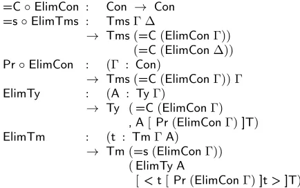
In contrast to the informal presentation of parametricity, here we have an additional judgement for types and we use de Bruijn indices instead of variable names which makes explicit weakening necessary. The motives for the eliminator are defined in figure 17.

We need to specify the fieldsConM_,TyM_,TmsM_andTmM_{in the}

record typeMotives. We construct these components separately as

Conm,Tym,TmsmandTmm.Conmspecifies what contexts will be

recordConm(Γ : Con) : Setwhere field

=C : Con

Pr : Tms =CΓ

Tym : ConmΓ → TyΓ → Set

TymΓMA = Ty(=CΓM, A[PrΓM]T)

recordTmsm(ΓM : ConmΓ) (∆M : Conm∆) (ρ : TmsΓ ∆) : Setwhere field

=s : Tms(=CΓM_{) (=C∆}M₎

PrNat : (Pr∆M_{)◦=s ≡ ρ◦(PrΓ}M₎

Tmm : (ΓM : ConmΓ) → TymΓMA → TmΓA → Set

Tmm_ΓM_AM_{a = Tm(=CΓ}M_{) (A}M_{[< a[PrΓ}M_{]t > ]T)}

M : Motives

M = record{ConM = Conm

;TyM = Tym

;TmsM = Tmsm

;TmM = Tmm}

Figure 17. Motives for the eliminator in the logical predicate in-terpretation

=C, but also to a weakening substitution Pr from the doubled

context to the original one. We put these together into a record

where=Cand Prare the projections, so if ΓM : ConM then

=CΓM : ConandPrΓM : Tms(=CΓM) Γ.

The motive for types receives the resultΓM of the eliminator

on the context and the type asAarguments. It will need to return

a type in the context =C ΓM extended with the type A(which

needs to be substituted by the projection). The predicate overA

is expressed by a type in a context extended with the domain of

the predicate. A substitutionρwill be mapped to the interpretation

=s which is between two doubled contexts and to a naturality

propertyPrNatwhich expresses that=scommutes withPr. This

property is used eg. to define the method for_[_]T, see below.

Terms will be mapped to terms in the doubled context and their type is the predicate at the original term (which has to be weakened

by Pr): this is expressed by substituting the type by the term

using<_>(defined in section 3). After defining the methods for

this interpretation, the eliminatorElimTmwill give us a proof of

parametricity for this theory:

=C◦ElimCon : Con → Con

=s◦ElimTms : TmsΓ ∆

→ Tms(=C(ElimConΓ))

(=C(ElimCon∆))

Pr◦ElimCon : (Γ : Con)

→ Tms(=C(ElimConΓ)) Γ

ElimTy : (A : TyΓ)

→ Ty (=C(ElimConΓ)

, A[Pr(ElimConΓ)]T)

ElimTm : (t : TmΓA)

→ Tm(=s(ElimConΓ))

(ElimTy A

[< t[Pr(ElimConΓ)]t > ]T)

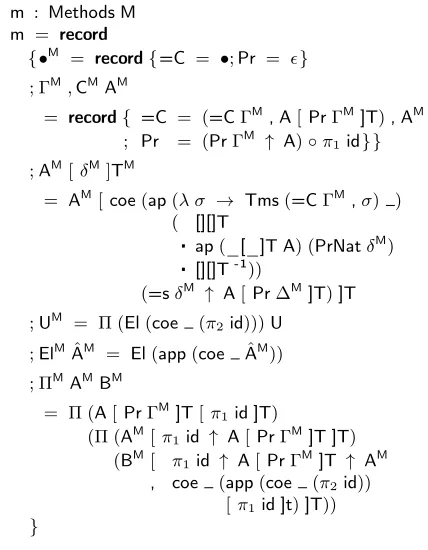
We list the methods for contexts and types as fields of the record

Methodsin figure 18. We omitted some implicit arguments and

used record syntax more liberally than Agda. The other methods

are straightforward but tedious to define due to the coercions that need to be performed. For details see the supplementary material.

The empty context is mapped to the empty context and the

empty substitution. The contextΓ , A is mapped to the doubled

context=CΓMforΓextended byAand the interpretationAM. The

projection substitution forΓ, Ajust projects out theAby lifting

PrΓMand is weakened so that it forgets about the additionalAM

in the context.

For deriving the interpretation of a typeA : Ty ∆

substi-tuted byδ : Tms Γ ∆we need to give a type in the context

=CΓM, A[ δ]T [PrΓM ]Tby the motive for types. The type

AMlives in the context=C∆M , A [ Pr∆M ]Tand by the

in-terpretation of the substitutionδand lifting overA[Pr∆M_]Tby

↑ we get

=sδM ↑ A[Pr∆M]T

: Tms(=CΓM, A[Pr∆M]T[=sδM]T) (=C∆M, A[Pr∆M]T).

We can substituteAM by=s δM ↑ A [ Pr ∆M ]Tbut still we

would get a type in the context

=CΓM, A[Pr∆M]T[=sδM]T

instead of

=CΓM_{, A[δ]T[PrΓ}M_]T.

However by the naturality rulePrNatδM

we know that

Pr∆M◦=sδM ≡ δ◦PrΓM.

With this in mind we can perform the following equality reasoning:

A[Pr∆M_]T[=sδM_]T

≡ h[][]T i

A[Pr∆M_◦=sδM_]T

≡ hap(_[_]T A) (PrNatδM_)i

A[δ◦PrΓM]T

≡ h[][]T-1 i

A[δ]T[PrΓM]T

Coercing=sδM ↑ A[Pr∆M ]Talong this equality (we denote

transitivity of equality by _ _) we get a substitution of the right

type

Tms(=CΓM, A[Pr∆M]T[=sδM]T)

(=C∆M_{, A[Pr∆}M_]T).

Similar coercions are taking place everywhere in the interpretation.

In the rest of the code-snippet we just write for the proofs of

equalities for the coercions. The interpretation ofUis like that of

Setin the informal presentation: predicates over the type

corre-sponding to the code in the last element of the context which can

be projected byπ2id. The predicate returns a code of a type inU.

The interpretation ofElgoes the opposite way: it takes the

predi-cateAM

fromAinto the universe and turns it into a predicate type

by first usingappto depend on the last element of the context and

then applyingElto get the type corresponding to the code. The

interpretation ofΠis the usual logical relation interpretation: we

are in the context=CΓM , Π A B [ PrΓM ]Tand we would

like to state that related arguments are mapped to related results by the function given in the last element of the context. We quantify

over the argument typeA(which needs to be weakened byPrΓM

because we are in an interpreted context, and by one step further

because of the last element in the context) and then overAMwhich

depends onAso the weakening here overΠA B[PrΓM]Tneeds

m : Methods M m = record

{•M

= record{=C = •;Pr = }

; ΓM_,CM_AM

= record{ =C = (=CΓM_{, A[PrΓ}M_]T),AM

; Pr = (PrΓM _{↑ A)◦π}

1id}}

;AM_[δM_]TM

= AM[coe(ap(λ σ → Tms(=CΓM,σ) )

( [][]T

ap(_[_]T A) (PrNatδM)

[][]T-1₎₎

(=sδM _{↑ A[Pr∆}M_]T)]T

;UM = Π (El(coe (π2id)))U

;ElMAˆM = El(app(coe AˆM))

; ΠMAMBM

= Π (A[PrΓM]T[π1id ]T)

(Π (AM[π1id ↑ A[PrΓM]T ]T)

(BM[ π1id ↑ A[PrΓM]T ↑ AM

, coe (app(coe (π2id))

[π1id ]t)]T))

}

Figure 18. Methods for specifying the logical predicate interpre-tation for contexts and types

in the context(=C(ΓM,CMAM), B[Pr(ΓM,CMAM)]T), the

first part of which is provided by the substitution

π1id ↑ A[PrΓM]T ↑ AM

: Tms(=CΓM,ΠA B[PrΓM]T

, A[PrΓM]T[π1id ]T

,AM_[π

1id ↑ A[PrΓM]T ]T)

(=CΓM_{, A[PrΓ}M_{]T ,A}M₎

which forgets the function from the context and is identity on the rest of the context and the second part is given by applying the function to the next element in the context and appropriately weakening and coercing the result.

Defining the logical predicate interpretation is tedious but fea-sible. Most of the work that needs to be done is coercing syntactic expressions using equality reasoning which can be simplified by using a heterogeneous equality [5] — two terms of different types are equal if there is an equality between the types and an equality between the terms up to this previous equality.

record_'_{A B : Set}(a : A) (b : B) : Set1where constructor_,_

field

projT : A ≡ B

projt : a≡[ projT ]≡b

_'_can be proven to be reflexive, symmetric and transitive so

equality reasoning can be done in the usual way. But it has the advantage that we can forget about coercions during reasoning:

uncoe : {a : A}(p : A≡’ B) → a'coe p a

Also, we can convert back and forth with the usual homogeneous equality:

from≡ : (p : A ≡ B) → a≡[ p ]≡b → a'b

to≡ : (p : a'b) → a≡[ projT p ]≡b

We note that the axiom of function extensionality was not used throughout the logical preciate interpretation.

5.3 The Eliminator for Closed Inductive-Inductive Types

An application of the logical predicate interpretation is to derive the syntax of the motives and methods for the eliminator of a closed inductive-inductive type.

A general closed inductive-inductive type has the following description in Agda notation:

dataA1 : T1 (signatures of types)

...

dataAn : Tn

dataA1where(constructors for A1)

c11 : A11

...

c1m1 : A1m1

...

dataAnwhere(constructors forAn)

cn1 : An1 ...

cnmn : Anmn

We haventypes and the typeAihasmiconstructors. Agda restricts

parameters of the constructors to only have strictly positive recur-sive occurrences of the type. The same restriction applies here.

First we note that the above description can be collected into the context where the variable names are the type names and construc-tor names, and they have the corresponding types:

•, A1 : T1, ...,An : Tn, c11 : A11, ...,c1m1 : A1m1 ,

...,cn1 : An1, ...,cnmn : Anmn

To define the motives and methods for the eliminator, we need a family over the types and fibers of that family over the constructors.

By applying the _Poperation to this context, the context is extended

by new elementsA1M, ...,AnMthe types of which are the motives

and by new elementsc11M , ...,cnmnMthe types of which will be

the methods, and they can be listed in a record:

recordMotives : Setwhere field

A1M : T1PA1 ...

AnM _{: Tn}P_An

recordMethods(M : Motives) : Setwhere

openMotives M

field

c11M : A11Pc11 ...

cnmn M

: Anmn P

cnmn

The method described here extends to types with equality con-structors by using the logical predicate interpretation of the equal-ity type. This is how we derived the motives and methods for the eliminator of the syntax.

6.

Homotopy Type Theory

may consider two types which have the same syntactic structure but which at some point use two different derivations to derive the same equality but these cannot be shown to be equal.

However, this can be easily remedied bytruncatingour syntax

to be a set, i.e. by introducing additional constructors:

setT : {A B : TyΓ} {e0 e1 : A ≡ B} → e0 ≡ e1

sets : {δ σ : TmsΓ ∆} {e0 e1 : δ ≡ σ} → e0 ≡ e1

sett : {u v : TmΓA} {e0 e1 : u ≡ v} → e0 ≡ e1

These force our syntax to be asetin the sense of HoTT, i.e. a type

for which UIP holds. We don’t need to do this forConbecause

this can be shown to be a set from the assumption thatTyare sets.

It seems to be entirely sensible to assume that the syntax forms a set, indeed we would want to show that equality is decidable which implies that the type is a set by Hedberg’s theorem [17].

However, we now run into a different problem: we can only eliminate into a type which is a set itself. That means that we cannot even define the standard model because we have to eliminate into Set1, the type of all small types, which is not a set in the sense of HoTT due to univalence, that is it has there may be more that one equality proof between two sets. One way around this would

be to replaceSet1 by an inductive-recursive universe, which can

be shown to be a set but for which univalence fails (see the formal development for the proofs).

dataUU : Set

EL : UU → Set

dataUUwhere

‘Π‘ : (A : UU) → (EL A → UU) → UU

‘Σ‘ : (A : UU) → (EL A → UU) → UU

‘>‘ : UU

EL(‘Π‘A B) = (x : EL A) → EL(B x)

EL(‘Σ‘A B) = Σ (EL A)λx → EL(B x)

EL‘>‘ = >

An apparent way around the limitation that we can only elim-inate into sets would be to only define the syntax in normal form and use a normalisation theorem. Since the normal forms do not require equality constructors there is no need to force the type to be a set and hence we could eliminate into any type. Indeed, this was proposed as a possible solution to the coherence problem in HoTT (e.g. how to define semi-simplicial types). However, it seems likely that this is not possible either. While we should be able to define the syntax of normal forms without equations we will need to incorpo-rate normalisation. An example would be the rule for application for normal forms:

$ : NeΓ (ΠA B) → (u : NfΓA)

→ NeΓ (B[< u > ]T)

Here we assume that we mutually define normal Nfand neutral

terms Ne and that all the types are in normal form. However,

a problem is the substitution appearing in the result which has to substitute a normal term into a normal type giving rise to a normal type. This cannot be a constructor since then we would have to add equalities to specify how substitution has to be behave. Hence we have to execute the substitution and at the same time normalize the result (this is known as hereditary substitution [28]). We may still think that this may be challenging but possible using an inductive-recursive definition. However, even in the simplest case, i.e. in a type theory only with variables we have to prove equational properties of the explicit substitution operation, which in turn appear in the proof terms, leading to a coherence problem which we have so far failed to solve.

Nicolai Kraus raised the question whether it may be possible to give the interpretation of a strict model like the standard model

(section 4) with the truncation even though we do not eliminate into a set. This is motivated by his work on general eliminations for the truncation operator [21]. Following this idea it may be possible to eliminate into set via an intermediate definition which states all the necessary coherence equations.

While defining the internal type theory as a set in HoTT seems to be of limited use, there are interesting applications in a 2-level theory similar to HTS as proposed by Voevodsky [32]. While the original proposal of HTS works in an extensional setting, it makes sense to consider a 2-level theory in an intensional setting

like Agda. We start with astricttype theory with uniqueness of

identity proofs (UIP) but within this we introduce a HoTT universe. This universe comes with its own propositional equality which is univalent but isn’t proof-irrelevant. From this equality we can only eliminate into types within the universe. We call the types

on the outsidepretypesand the types in the universetypes. The

construction of the type-theoretic syntax takes place on the level of pretypes which is compatible with our assumption of UIP. On the other hand we can eliminate into the HoTT universe which is univalent. In this setting definitional equalities are modelled by strict equality and propositional equality by the univalent equality within the universe. Our definition of the syntax takes place at the level of pretypes but when constructing specific interpretations we eliminate into types.

7.

Discussion and Further Work

We have for the first time presented a workable internal syntax of dependent type theory which only features typed objects. We have shown that the definition is feasible by constructing not only the standard model but also the logical predicate interpretation. Further interpretations are in preparation, e.g. the setoid interpretation and the presheaf interpretation. The setoid interpretation is essential for a formal justification of QITs and the presheaf interpretation is an essential ingredient to extend normalisation by evaluation [4] to de-pendent types. These constructions for dede-pendent types require an attention to detail which can only convincingly demonstrated by a formal development. At the same time this approach would give us a certified implementation of key algorithms such as normalisation. Clearly, we have only considered a very rudimentary type the-ory here, mainly for reasons of space. It is quite straightforward to

add other type constructors, e.g.Σ-types, equality types, universes.

We also would like to reflect our very general syntax for inductive-inductive types and QITs but this is a more serious challenge.

Having an internal syntax of type theory opens up the exciting

possibility of developingtemplate type theory. We may define an

interpretation of type theory by defining an algebra for the syntax and the interpretation of new constants in this algebra. We can then interpret code using these new principles by interpreting it in the given algebra. The new code can use all the conveniences of the host system such as implicit arguments and definable syntactic extensions. There are a number of exciting applications of this approach: the use of presheaf models to justify guarded type theory has already been mentioned [20]. Another example is to model the local state monad (Haskell’s STM monad) in another presheaf category to be able to program with and reason about local state and other resources. In the extreme such a template type theory may allow us to start with a fairly small core because everything else can be programmed as templates. This may include the computational explanation of Homotopy Type Theory by the cubical model — we may not have to build in univalence into our type theory.

Acknowledgments

the pure version of internal type theory. We would also like to thank Paolo Capriotti, Gabe Dijkstra and Nicolai Kraus for discussions and work related to the topic of this paper, in particular questions related to HITs and coherence problems. We are also grateful to the anonymous reviewers for their helpful comments and suggestions.

References

[1] nlab: Beck-chevalley condition. Available online. Accessed: 2015-10-26.

[2] The Agda Wiki, 2015. Available online.

[3] T. Altenkirch and A. Kaposi. Supplementary material for the paper Type Theory in Type Theory using Quotient Inductive Types, 2015. Available online at the second author’s website.

[4] T. Altenkirch, M. Hofmann, and T. Streicher. Categorical reconstruc-tion of a reducreconstruc-tion free normalizareconstruc-tion proof. In D. Pitt, D. E. Ry-deheard, and P. Johnstone, editors,Category Theory and Computer Science, LNCS 953, pages 182–199, 1995.

[5] T. Altenkirch, C. McBride, and W. Swierstra. Observational equality, now! InPLPV ’07: Proceedings of the 2007 workshop on Program-ming languages meets program verification, pages 57–68, New York, NY, USA, 2007. ACM. ISBN 978-1-59593-677-6. .

[6] T. Altenkirch, P. Morris, F. N. Forsberg, and A. Setzer. A categorical semantics for inductive-inductive definitions. InCALCO, pages 70– 84, 2011.

[7] J.-P. Bernardy, P. Jansson, and R. Paterson. Proofs for free — para-metricity for dependent types. Journal of Functional Programming, 22(02):107–152, 2012. .

[8] M. Bezem, T. Coquand, and S. Huber. A model of type theory in cubical sets. In19th International Conference on Types for Proofs and Programs (TYPES 2013), volume 26, pages 107–128, 2014.

[9] E. Brady. Idris, a general-purpose dependently typed programming language: Design and implementation. Journal of Functional Pro-gramming, 23:552–593, 2013. ISSN 1469-7653. .

[10] M. Brown and J. Palsberg. Self-representation in Girard’s System U.

SIGPLAN Not., 50(1):471–484, Jan. 2015. ISSN 0362-1340. .

[11] J. Cartmell. Generalised algebraic theories and contextual categories.

Annals of Pure and Applied Logic, 32:209–243, 1986.

[12] J. Chapman. Type theory should eat itself. Electron. Notes Theor. Comput. Sci., 228:21–36, Jan. 2009. ISSN 1571-0661. .

[13] N. Danielsson. A formalisation of a dependently typed language as an inductive-recursive family. In T. Altenkirch and C. McBride, editors,

Types for Proofs and Programs, volume 4502 ofLecture Notes in Computer Science, pages 93–109. Springer Berlin Heidelberg, 2007. ISBN 978-3-540-74463-4.

[14] D. Devriese and F. Piessens. Typed syntactic meta-programming. In

Proceedings of the 2013 ACM SIGPLAN International Conference on Functional Programming (ICFP 2013), pages 73–85. ACM, Septem-ber 2013. ISBN 978-1-4503-2326-0. .

[15] R. Diaconescu. Axiom of choice and complementation.Proceedings of the American Mathematical Society, 51(1):176–178, 1975.

[16] P. Dybjer. Internal type theory. InTypes for Proofs and Programs, pages 120–134. Springer, 1996.

[17] M. Hedberg. A coherence theorem for Martin-Löf’s type theory.

Journal of Functional Programming, 8(04):413–436, 1998.

[18] M. Hofmann.Extensional Concepts in Intensional Type Theory. The-sis. University of Edinburgh, Department of Computer Science, 1995.

[19] M. Hofmann. Syntax and semantics of dependent types. In Exten-sional Constructs in IntenExten-sional Type Theory, pages 13–54. Springer, 1997.

[20] G. Jaber, N. Tabareau, and M. Sozeau. Extending type theory with forcing. InLogic in Computer Science (LICS), 2012 27th Annual IEEE Symposium on, pages 395–404. IEEE, 2012.

[21] N. Kraus. Truncation Levels in Homotopy Type Theory. PhD thesis, University of Nottingham, 2015.

[22] D. Licata. Running circles around (in) your proof assistant; or, quo-tients that compute, 2011. Available online.

[23] C. McBride. Dependently Typed Functional Programs and their Proofs. PhD thesis, University of Edinburgh, 1999.

[24] C. McBride. Outrageous but meaningful coincidences: dependent type-safe syntax and evaluation. In B. C. d. S. Oliveira and M. Za-lewski, editors,Proceedings of the ACM SIGPLAN Workshop on Generic Programming, pages 1–12. ACM, 2010. ISBN 978-1-4503-0251-7. .

[25] N. Mendler. Quotient types via coequalizers in Martin-Löf type theory. InProceedings of the Logical Frameworks Workshop, pages 349–361, 1990.

[26] F. Nordvall Forsberg. Inductive-inductive definitions. PhD thesis, Swansea University, 2013.

[27] U. Norell. Towards a practical programming language based on de-pendent type theory. PhD thesis, Chalmers University of Technology, 2007.

[28] F. Pfenning. Church and curry: Combining intrinsic and extrinsic typing. 2008.

[29] A. Pitts. Quotient types in Agda. Private email, May 2015.

[30] J. C. Reynolds. Types, abstraction and parametric polymorphism. In R. E. A. Mason, editor,Information Processing 83, Proceedings of the IFIP 9th World Computer Congress, pages 513–523. Elsevier Science Publishers B. V. (North-Holland), Amsterdam, 1983.

[31] The Univalent Foundations Program. Homotopy type theory: Univa-lent foundations of mathematics. Technical report, Institute for Ad-vanced Study, 2013.