An extended ANFIS architecture and its learning properties for type 1 and interval type 2 models

An Extended ANFIS Architecture and its Learning

Properties for Type-1 and Interval Type-2 Models

Chao Chen

, Robert John

, Jamie Twycross

, Jonathan M. Garibaldi

University of Nottingham

Email:{∗psxcc4,†robert.john,‡jamie.twycross,§jon.garibaldi}@nottingham.ac.uk

Abstract—In this paper, an extended ANFIS architecture is proposed. By incorporating an extra layer for the fuzzification process, the extended architecture is able to fit both type-1 and interval type-2 models. The learning properties of the proposed architecture based on the least-squares estimate method are studied on selected type-1 and interval type-2 ANFIS models. We show that the least-squares estimate method in general behaves differently for interval 2 ANFIS models compared to type-1 ANFIS models, producing larger errors for interval type-2 ANFIS.

I. INTRODUCTION

A common concern for constructing a fuzzy inference system (FIS) is that there are no standard methods for trans-forming human knowledge or experience into the rule base. Also, effective methods are required to tune the membership functions for optimising the performance of FISs. The ar-chitecture of Adaptive-Network-based Fuzzy Inference System (ANFIS) was proposed by Jang [1] to serve as a basis for constructing a set of fuzzy rules with appropriate MFs to generate the stipulated FIS. The original ANFIS was designed for type-1 (T1) Takagi-Sugeno-Kang (TSK) inference models. A hybrid learning algorithm based on the gradient method and the least-squares estimate (LSE) is applied to identify parameters.

An increasing interest in type-2 (T2) fuzzy systems has led to an increase in research on interval T2 (IT2) ANFIS. For example, early studies on T2 ANFIS can be found in [2, 3], who reported an approach that uses an adaptive network to learn a T2 fuzzy system based on linguistic inputs and numeric output. Other examples for research on T2 ANFIS, based on crisp inputs, can be found in [4, 5, 6, 7, 8, 9]. It has been proposed that least-squares based methods cannot be applied to a T2 fuzzy logic system (FLS) Mendel [10], since the Fuzzy Basis Function expansion for a T2 TSK FLS, which is the starting point for the LSE method, cannot be obtained without knowing the consequent parameters in advance. This issue was also concluded in [5] and addressed by giving initialised consequent parameters. In their study, it was proposed that convergence of the hybrid learning algorithms based on the recursive least-squares and the back-propagation (BP) methods can be obtained in practice. As an extension of the studies on ANFIS based on singleton fuzzification, studies on non-singleton fuzzification based IT2 ANFIS can be found in [7, 11, 12].

Though some studies has been made on IT2 ANFIS, a clear architecture for IT2 ANFIS has not been presented in literature compared to that of T1 ANFIS presented in [1]. In this paper, an extended architecture of ANFIS is proposed and clearly presented. By incorporating an extra layer for the fuzzification process, the extended architecture fits both T1 and IT2 models. The inappropriateness of the LSE algorithm for IT2 ANFIS, as mentioned by Mendel [10], is investigated in detail. The properties of the hybrid learning algorithms BP-LSE are studied on selected T1 and IT2 ANFIS models. Through both an analytical and practical exploration, we show that the LSE method does not behave in the same way for IT2 ANFIS compared to T1 ANFIS.

II. AN EXTENDED ARCHITECTURE OFANFIS

x1

x2

F

F

Sup

Sup

Sup

Sup A1

A2

A3

A4

N

N

N

N

C1

C2

C3

C4

_y

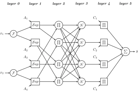
layer 0 layer 1 layer 2 layer 3 layer 4 layer 5

Fig. 1. An example of the extended ANFIS architecture, where the symbolF denotes the operation of fuzzification.Supinlayer 1denotes the operation of getting the membership grades for given inputs and antecedents. The symbols

,N anddenote production, normalisation and summation respectively.

(FSs). Afterwards, the membership grades of the crisp inputs can be obtained in layer 1. The use of layer 0 makes the fuzzification process clearer, especially when non-singleton fuzzification is applied. Also, the extended architecture of ANFIS is suitable for both T1 and IT2 ANFIS.

In the example of the extended ANFIS architecture, there are four fuzzy inferencing rules (TSK type) with two inputs (x₁,x₂) and one output (y). Specifically, the inferencing rules are:

IFx₁ isA₁ ANDx₂ isA₃,THENf₁is C₁ IFx₁ isA1 ANDx2 isA4,THENf₂is C2 IFx₁ isA₂ ANDx₂ isA₃,THENf₃is C₃ IFx₁ isA₂ ANDx₂ isA₄,THENf₄is C₄

where A₁, A₂ and A₃, A₄ are the antecedent membership functions for inputx₁andx₂respectively.Ciis the consequent

linear function for the outputfiof theithrule,i∈ {1,2,3,4}.

It should be noted thatfi is the output of each fuzzy rule and

y is the output of the ANFIS. Specifically, y is the weighted average of all the fi.

A. T1 ANFIS

For T1 ANFIS, all the antecedents are T1 FSs. For example, A1 in the rule above can be represented as x∈X1μA1(x)/x where X₁ is the universe of the primary variable x₁. The consequents can be either constants or linear functions. The most commonly used consequent representation is the first-order linear function which can be defined as:

Ci≡fi=pi+qix1+rix2

wherepi, qi, riare the coefficients of the linear functions, and

they will be referred to as consequent parameters.

a) Layer 0: Every nodei in this layer is a fuzzifier, for which the input is a crisp number and the output O_Li₀ is a T1 FS Fi. The fuzzification method can be either singleton

or T1 non-singleton. In the literature, most of the T1 ANFIS research and applications are based on singleton fuzzification, while T1 non-singleton is rarely used and can be seen in [13]. b) Layer 1: Every node i in this layer has two inputs, the fuzzy input Fj (the output from the corresponding node

of layer 0) and the corresponding antecedent FS Ak. The

output of node i is the maximum membership grade of the intersection of Fj andAk. It can be represented as:

Oi

L1 = supFj∩Ak

For example, for the first node of layer 1 in Fig. 1, Fj is F1 andAk isA1. Then,

O1

L1 = sup

x∈X1

μF1(x) μA1(x)

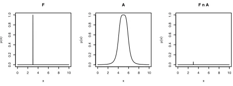
where is the t-norm operation which can be either min or prod. It should be noted that the calculation in this layer is different from [1] where singleton fuzzification is used. Two examples are given in Figs. 2 and 3 to illustrate Fj∩Ak for

singleton and non-singleton fuzzification respectively.

0 2 4 6 8 10

0.0 0.2 0.4 0.6 0.8 1.0 F x μ ( x )

0 2 4 6 8 10

0.0 0.2 0.4 0.6 0.8 1.0 A x μ ( x )

0 2 4 6 8 10

0.0 0.2 0.4 0.6 0.8 1.0

F n A

x

μ

(

x

)

Fig. 2. An illustration of F ∩Abased on the min operator, where F denotes the fuzzy input generated by singleton fuzzification and_Adenotes the antecedent FS.

0 2 4 6 8 10

0.0 0.2 0.4 0.6 0.8 1.0 F x μ ( x )

0 2 4 6 8 10

0.0 0.2 0.4 0.6 0.8 1.0 A x μ ( x )

0 2 4 6 8 10

0.0 0.2 0.4 0.6 0.8 1.0

F n A

x

μ

(

x

)

Fig. 3. An illustration ofF∩Abased on theminoperator, whereFdenotes the fuzzy input generated by non-singleton fuzzification andAdenotes the antecedent FS.

c) Layer 2 to 5: The calculations from layer 2 to 5 are the same as that defined in [1]. Thus, these layers are not explained here in detail. Only the formulas for the outputs of nodes in these layers are given below:

Oi

L2 ≡ wi=O j L1O

k L1

Oi

L3 ≡ wi =

Oi L2

₄

j=1OLj2

Oi

L4 = O

i

L3Ci=wifi

OL5 ≡ y= 4

i=1 Oi

L4

B. IT2 ANFIS

According to the definition of T2 fuzzy logic systems by Karnik et al. [14], if there exists a IT2 FS in the antecedent or consequent MFs of an ANFIS, then such an ANFIS can be called as IT2 ANFIS. For simplicity, in this paper, all the antecedents are IT2 FSs. For example, A₁ in the rule above can be represented as two T1 MFs, which are lower MF

¯ A1 and upper MF A¯₁. The consequent linear functions can also be defined as intervals such as

¯

C1,C¯1forC1 in Fig. 1. For example, as an equivalent representation in [12],

¯ Ci,C¯i

for Ci can be defined as:

¯ Ci≡

¯fi=pi+qix1+rix2−si−ti|x1| −ui|x2|

¯

Ci≡f¯i=pi+qix1+rix2+si+ti|x1|+ui|x2|

It should be noted that the limitation for the above definition is that si, ti and ui should be no less than zero in order

to guarantee that f¯i is no less than

¯

consequent linear functions can be the same as that defined for T1 ANFIS above. In this case, f¯i is equal to

¯fi.

a) Layer 0: Similar to T1 ANFIS, every nodei in this layer is a fuzzifier. However, the fuzzification method can be singleton [5], T1 singleton [7, 12], as well as IT2 non-singleton[11, 15]. Thus, the output Oi

L0 can be either a T1 FS or a IT2 FS. For example, if IT2 non-singleton is used for nodei, thenOi_L0 is a IT2 FSFi, which can be represented as

a lower MF ¯

Fi and a upper MFF¯i. If singleton or T1

non-singleton fuzzification is used, the output Oi_L0 is a T1 FS. However, to be simple, such a T1 FS can also be considered as a special IT2 FS for which

¯

Fi is the same asF¯i.

b) Layer 1: In this layer, the outputOi

L1 of node iis a interval

¯ Oi

L1,O¯ i

L1 , where:

¯ Oi

L1 = sup_¯Fj∩A_¯k

¯ Oi

L1 = sup ¯Fj∩A¯k

For example, for the first node of layer 1 in Fig. 1, Fj is F1 andAk isA1. Then,

¯ O1

L1 = sup

x∈X1

μ ¯

F1(x) μ_¯A1(x)

¯ O1

L1 = sup

x∈X1

μF¯1(x) μA¯1(x)

c) Layer 2: The operation in this layer is similar to that for T1 ANFIS. The difference is that wi here is an interval

which can be represented as [ ¯

wi,w¯i]. For instance, the output

of the first node in this layer can be represented as:

¯ O1

L2≡w_¯1=O_¯1L1O_¯3L1

¯ O1

L2≡w¯1= ¯O1L1O¯3L1

d) Layer 3: Before normalising the firing strengths ob-tained inlayer 2, a single firing strengthw_i should be selected for each nodei. Theoretically, there are infinite combinations of firing strengths and thus it is impossible to select and compute all of the possible combinations. In practice, two representative combinations are commonly used for approxi-mations. In [9], all the

¯

wiare used as one combination and all

thew¯iare used as another combination. The approach used by

Mendez and Juarez [5] is based on the KM algorithms [16]. It will be explained later that the output of layer 5 for IT2 ANFIS is constituted of

¯

OL5andO¯L5. It is defined thatw_¯i is

the selected in one combination for ¯

OL5, andw¯i is selected in

another combination for ¯

OL5, where_¯wi,w¯i ∈[w_¯i,w¯i]. Then,

the outputOi

L3 can be represented asO_¯ i

L3 andO¯ i

L3, where:

¯ Oi

L3 ≡w_¯i= ¯

w i

₄

j=1w_¯j

¯ Oi

L3 ≡w¯i=

¯ w

i

₄

j=1w¯j

It should be noted that ¯ w

i does not necessarily need to be

smaller thanw¯_i. Also, ¯ Oi

L3 (w_¯i) does not necessarily need to

be smaller than O¯i L3 (w¯i).

e) Layer 4: The outputOi_L4 of theithnode in this layer can be represented as

¯ Oi

L4 andO¯ i

L4, where:

¯ Oi

L4 =w_¯i

¯

fi=O_¯iL3C_¯i

¯ Oi

L4 = ¯wif¯i= ¯O i L3C¯i

It should also be noted that ¯ Oi

L4 does not necessarily need to be smaller thanO¯i

L4.

f) Layer 5: OL5, which is the final output y, is consti-tuted of

¯

OL5 andO¯L5. These can be represented as: OL5≡y=qO_¯L5+ (1−q) ¯OL5

where

¯ OL5=

4

i=1¯

Oi L4 =

4

i=1¯

wi

¯ fi

¯ OL5=

4

i=1 ¯ Oi

L4 = 4

i=1 ¯ wif¯i

and as presented in [9], q is a constant, which is usually set to be 0.5 [12]. It should be noted that

¯

OL5is guaranteed to be no larger than

¯

OL5 if the selection approach in layer 3is based on the KM algorithms. In contrast, this cannot be guaranteed in [9].

III. THE LEARNING ALGORITHMS OFANFIS

The learning algorithms of ANFIS are usually related to methods for updating the antecedent parameters and conse-quent parameters during the training process. Though not found in the literature, it is also possible to learn the param-eters for fuzzification.

The back-propagation based on the gradient descent meth-ods and the LSE algorithm are commonly used as the learning algorithms for updating the parameters [1]. Recursive square-root filters (REFIL) and orthogonal least-squares (OLS) al-gorithms are used in [11, 12] for learning the consequent parameters. Some other algorithms such as Particle Swarm Optimisation (PSO) and the Sliding Mode Control (SMC) approach are also reported as learning algorithms for IT2 ANFIS [17, 9]. The remains of this section are focused on the LSE algorithm, which has been proposed to be inappropriate for IT2 ANFIS [10].

A. Linear equation for T1 ANFIS

For a single entry of the training data, it is observed that the final outputyof T1 ANFIS described in Section II-A can be represented as:

y=Xθ

whereX andθ are vectors which can be represented as:

X = w1 w1x1 w1x2 ... w4 w4x1 w4x2 θT _{= p}

X = w¯1+ ¯w1

2 ¯

w₁+ ¯w1

2 x1 ¯

w₁+ ¯w1

2 x2 ... ¯

w₄+ ¯w4

2 ¯

w₄+ ¯w4

2 x1 ¯

w₄+ ¯w4 2 x2

(1) θT _{= p}

1 q1 r1 ... p4 q4 r4 (2)

B. Linear equation for IT2 ANFIS

For simplicity, the consequent linear functions for IT2 ANFIS are defined to be the same as those for T1 ANFIS above. Then, for a single entry of the training data, the final output y of IT2 ANFIS described above can also be represented as:

y=Xθ

where X and θ are vectors which can be represented as Equation 1 and 2 (supposing the coefficient q for OL5 is set to be 0.5).

It should be noted that, if the KM algorithms are applied, θshould firstly be initialised in order to obtain the matrixX by properly selecting the rule firing strengths from the output interval [

¯

wi,w¯i]for each node iinlayer 2.

The consequent linear functions can also be easily defined to be intervals as

¯

C,C¯. However, during the training process, it should be assured that

¯

C is no larger thanC¯. For example, as mentioned in Section II-B, b should be no less than zero for the defined consequent intervals.

C. LSE and its inappropriateness for IT2 ANFIS

For multiple entries of the training data, the output Y for both T1 and IT2 ANFIS can be represented as the following matrix equation:

Y =Xθ

Hence, given the input matrix X and the output Y, the parameters θ can be easily estimated by the LSE algorithm. For T1 ANFIS, the estimatedθcan fit the training data with an optimised training error, which is the same as the estimation error (residual) obtained by the LSE. However, it should be noted that the LSE algorithm cannot guarantee an optimised training error for IT2 ANFIS. This is because the estimation error for IT2 ANFIS obtained by the LSE algorithm will almost certainly be different from the final training error for the training data. To clearly illustrate this issue, the estimation errore and the training errore are defined as:

e_{=Y −Xθ}

e_{=Y −Xθ}

where θ is estimated by the LSE algorithm with the input X _{and the output Y. It should be noted that when the same} training data are used to validate the estimatedθ, the outputY does not change for calculatinge. However, the input matrix could change and hence it is defined as X.

Specifically, for T1 ANFIS, X is the same as X. Thus, e _{will be exactly the same ase. This means, for T1 ANFIS,}

the training error is the estimation error obtained by the LSE algorithm for the training data.

However, the situation for IT2 ANFIS is different from that for T1 ANFIS. For IT2 ANFIS, X is determined by the initialised θ when the KM algorithms are applied for selecting the representative firing strengths in layer 2. After applying the LSE algorithm, the consequent parameters will be updated toθ, which is optimised for the input matrix X. It should be noted thatθwill almost certainly be different from the initialisedθ. Thus, when the same training data are then used in the validation process, the input matrixX, which is determined by the new parametersθ, will almost certainly be different from the input matrixX used by the LSE algorithm. For example,

¯

w₁ could be w¯1 ¯

w1+ ¯w2+ ¯w3+ ¯w4 for X

_{, while it}

may be ¯w1 ¯

w1+_¯w2+w_¯3+w_¯4 for X

_{. Accordingly, e will almost}

certainly be different frome for IT2 ANFIS. This means, θ is optimised by the LSE algorithm for X and Y. However, it does not fit X as well as it fits X. In other words, for IT2 ANFIS, the LSE method cannot be used to guarantee an optimised training error for the training data when the KM algorithms are applied for selecting the representative firing strengths inlayer 2.

IV. EVALUATION

In Section III, we discussed how the LSE method can be applied to T1 ANFIS to obtain an optimised error for the training data. However, such optimised error cannot be obtained by the LSE method in IT2 ANFIS in the same way as that in T1 ANFIS. In this section, we use the classification problem with the IRIS data [18] to further investigate this issue in practice.

In our testing models, five fuzzy rules are used where petal length (x₁) and petal width (x₂) are inputs, and species (C) are outputs. Each input has three MFs. Specifically, the five rules are:

IFx₁ isAx1,low AND x2 isAx2,low,THEN C1

IF x₁ isAx1,mid ANDx2 isAx2,mid,THEN C2 IFx₁ isAx1,high AND x2 is Ax2,high,THEN C3

IFx₁ isAx1,midAND x2 is Ax2,high,THEN C4 IFx₁ isAx1,high ANDx2 isAx2,mid,THEN C5

A. Training with pure LSE

To clearly show how the LSE method works in T1 and IT2 ANFIS models, only the LSE method are used to tune the consequent parameters. The antecedent MFs are arbitrarily initialised and then are fixed during the training process. All the 150 instances of the IRIS data are used as the training data. The estimation errore and the training erroredefined in Section III-C are examined during the training epochs with both batch and online training modes. With the batch mode, parameters are updated only after the whole training data set has been presented for each epoch. On the other hand, with the online mode, parameters are updated immediately after each input-output pair of training data within each epoch.

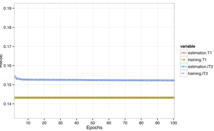
For the batch training mode, the results are shown in Fig. 4. It can be observed that the relevant estimation and training errors by the T1 model are the same. However, clear differences can be identified between the estimation and training errors by the IT2 model. Also, the errors obtained by the T1 ANFIS model do not change during the training epochs, while the errors by the IT2 ANFIS model fluctuate. No clear error convergence can be found in this figure. Some of the estimation errors by the IT2 ANFIS model are smaller than the relevant estimation errors by the T1 ANFIS model. However, almost all the training errors by the IT2 ANFIS model are larger than the training errors by the T1 ANFIS model.

The results of online mode are shown in Fig. 5. It can be noticed the results of T1 ANFIS with online mode are the same to those with the batch mode above. However, the IT2 model performs differently with online mode. Although the differences between estimation and training errors obtained by the IT2 ANFIS model still exist, they cannot be clearly identified especially after a couple of training epochs. Though not clear, error convergence can be found for the IT2 model. However, all the errors obtained by the IT2 ANFIS model are larger than those produced by the T1 ANFIS model.

B. Training with BP-LSE

More tests have been made with BP-LSE, as the hybrid learning algorithm, to further examine how the LSE method performs incorporating the gradient method for T1 and IT2 ANFIS models. Specifically, the parameters in Layer 2 are updated by the BP algorithm and the parameters in Layer 4 are estimated by the LSE method. The results are shown in Figs. 6 and 7 for batch and online training modes respectively. In batch mode, the estimation and training errors for each epoch for T1 ANFIS are still the same. However, it should be noted that such consistency disappears when the T1 ANFIS model is trained in online mode. In contrast, clear differences between estimation and training errors for IT2 ANFIS can be observed in both batch and online modes.

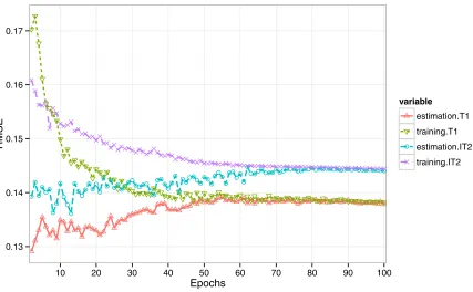
With BP-LSE, fluctuations can be clearly observed from all the errors except that obtained by the T1 model in the batch mode. However, all the errors converge during the training epochs. It can be observed that, in this case, the T1 ANFIS model still gives smaller errors than the IT2 ANFIS model after a couple of training epochs.

V. DISCUSSION

An IT2 ANFIS can be considered as a combination of all possible embedded T1 ANFIS. According to the definition in Section II-B, the output of IT2 ANFIS is in fact the output of its representative embedded T1 ANFIS, which is determined by the consequent parameters if the KM algorithms are applied for selecting the representative firing strengths. Thus, the optimisation of an IT2 ANFIS is in fact the optimisation of the representative T1 ANFIS.

As can be clearly observed from our results, the training errors by IT2 ANFIS are generally larger than the corre-sponding estimation errors. This is because the estimation errors are least square errors optimised by the LSE method for the selected representative embedded T1 ANFIS. However, as discussed in Section III-C, since the consequent parameters are updated after LSE optimisation, the representative embedded T1 ANFIS will also be changed. Hence, the updated conse-quent parameters do not fit the new representative embedded T1 ANFIS. As a result, the training errors will generally be larger than the estimation errors.

It should be noted that when the hybrid learning algorithm (BP-LSE) is applied in online mode, the estimation errors are also not equal to the training errors for T1 ANFIS (see Fig. 7). This is because the antecedent parameters are updated within each epoch for every entry of the training data. This makes X_{different fromXwhen errors are checked after all entries} of the training data are learned for each learning epoch.

In Fig. 7, it is also interesting to note that the estimation errors gradually increase during the training epochs. This is a special property of the LSE method in online training mode. The BP-LSE algorithm in online mode does not guarantee an optimised fit for the training data. Therefore the estimation errors for T1 ANFIS in Fig. 7 are larger than that in Fig. 6.

In Figs. 4 and 6, errors obtained by IT2 ANFIS during the training epochs show more fluctuation than errors obtained by T1 ANFIS. The fluctuation of errors is in essence related to the change of the matrix X during the training epochs. For T1 ANFIS, the change of the matrixX is only related to the change of antecedent parameters. However, for IT2 ANFIS, it is related to the change of both the antecedent and the consequent parameters. Thus, the change of matrixX for IT2 ANFIS is potentially larger than that for T1 ANFIS. Thus, the larger change of the matrixX leads to the larger fluctuation. This is also the reason for the smaller error fluctuations seen in online mode compared to batch mode: the change of parameters in online mode is relatively smaller than that in batch mode.

●

●●

●

●

●●●●_●

● ●

● ●●●

● ●

● ●

●

●●

●

●●●●●●●●●●

● ●

●

● ●

●●●●●●●●

● ●

●

● ●

●●●●●●●●

● ●

●

● ●

●●●●●●●●

● ●

●

● ●

●●●●●●●●

● ●

●

● ●

●●●●●●●●

0.14 0.15 0.16 0.17 0.18 0.19

10 20 30 40 50 60 70 80 90 100

Epochs

RMSE

variable

●

estimation.T1

training.T1

estimation.IT2

training.IT2

Fig. 4. The estimation and training error curves for the training data during the pure LSE training epochs with IRIS data (batch mode)

●

●●●●●●●●●●●●●●●●●●●●●●●●●●●●●●●●●●●●●●●●●●●●●●●●●●●●●●●●●●●●●●●●●●●●●●●●●●●●●●●●●●●●●●●●●●●●●●●●●●

0.14 0.15 0.16 0.17 0.18 0.19

10 20 30 40 50 60 70 80 90 100

Epochs

RMSE

variable

●

estimation.T1

training.T1

estimation.IT2

training.IT2

●●●

●●●●_●

● ●

● ●

●●●●_●●●

●●●●●●●●●●_{●●●●●●●●}

● ●●●●

●●●●●●●_●●●●●●●●●

● ●

●

●●●●

●

●●●●

● ●

●●●●

● ●

●●●●_●●_●●●●

●●●●

●_●

●

●_●

● ●

0.125 0.150 0.175

10 20 30 40 50 60 70 80 90 100

Epochs

RMSE

variable

●

estimation.T1

training.T1

estimation.IT2

training.IT2

Fig. 6. The estimation and training error curves for the training data during the hybrid (BP-LSE) training epochs with IRIS data (batch mode)

● ●

● ●

●●

● ●

●

● ●

● ●

●

●●

●

●●_●

●

●●_●●●●●●●●●●

● ●

●●_●

●●

●

●

●●●●●●●●●

●●●

● ●●

●●

● ●

●●●●●●●●●●●●●●●●●●●●●●●●●●●●●●●●●●●●●●

0.13 0.14 0.15 0.16 0.17

10 20 30 40 50 60 70 80 90 100

Epochs

RMSE

variable

●

estimation.T1

training.T1

estimation.IT2

training.IT2

that the LSE method is not appropriate for IT2 ANFIS when the KM algorithms are applied for selecting the representative firing strengths in layer 2.

VI. CONCLUSION

We have presented an extended six-layer ANFIS architec-ture suited to both T1 and IT2 ANFIS. By incorporating an extra layer, the fuzzification process is explicitly addressed compared to the original five-layer architecture. Both singleton and non-singleton fuzzification methods are supported by our extended architecture. Through a detailed discussion, we have shown that the LSE method does not exhibit the same behaviour for KM-based IT2 ANFIS compared to T1 ANFIS. This is supported in practice through results presented on the IRIS classification problem. In our evaluation, T1 ANFIS models generally produce smaller errors than IT2 ANFIS models when they are trained by either the pure LSE or the hybrid BP-LSE algorithms. Thus, we conclude that the LSE method is not generally suitable as the training algorithm for IT2 ANFIS models when the KM algorithms are applied for selecting the representative firing strengths in layer 2. However, a simple data set is obviously not enough, the results need to be verified with more data sets in the future. On the other hand, we are currently exploring alternatives to the KM algorithms, such as the Nie-Tan method [19], which would allow the LSE method to be used for IT2 ANFIS models.

REFERENCES

[1] J.-S. Jang, “ANFIS: adaptive-network-based fuzzy infer-ence system,”IEEE Transactions on Systems, Man, and Cybernetics, vol. 23, no. 3, pp. 665–685, 1993.

[2] R. I. John and C. Czarnecki, “A type 2 adaptive fuzzy inferencing system,” inProceedings IEEE International Conference on Systems, Man, and Cybernetics, vol. 2, 1998, pp. 2068–2073.

[3] R. I. John and C. Czarnecki, “An adaptive type-2 fuzzy system for learning linguistic membership grades,” in Proceedings IEEE International Conference on Fuzzy Systems, vol. 3, 1999, pp. 1552–1556.

[4] G. M. Mendez and O. Castillo, “Interval type-2 TSK fuzzy logic systems using hybrid learning algorithm,” inProceedings IEEE International Conference on Fuzzy Systems, 2005, pp. 230–235.

[5] G. Mendez and I. Juarez, “First-order interval type-2 TSK fuzzy logic systems using a hybrid learning algorithm,” WSEAS Transactions on Computers, vol. 4, no. 4, pp. 378–384, 2005.

[6] G. Mendez and M. De Los Angeles Hernandez, “Interval Type-2 ANFIS,” in Innovations in Hybrid Intelligent Systems, E. Corchado, J. Corchado, and A. Abraham, Eds. Springer Berlin Heidelberg, 2007, vol. 44, pp. 64– 71.

[7] G. Mendez and M. Hernandez, “Interval type-1 non-singleton type-2 fuzzy logic systems are type-2 adaptive neuro-fuzzy inference systems.”International Journal of

Reasoning-based Intelligent Systems, vol. 2, no. 2, pp. 95–99, 2010.

[8] M. A. Khanesar, E. Kayacan, M. Teshnehlab, and O. Kaynak, “Extended Kalman Filter Based Learning Algorithm for Type-2 Fuzzy Logic Systems and Its Ex-perimental Evaluation,”IEEE Transactions on Industrial Electronics, vol. 59, no. 11, pp. 4443–4455, 2012. [9] E. Kayacan, O. Cigdem, and O. Kaynak, “Sliding Mode

Control Approach for Online Learning as Applied to Type-2 Fuzzy Neural Networks and Its Experimental Evaluation,” IEEE Transactions on Industrial Electron-ics, vol. 59, no. 9, pp. 3510–3520, 2012.

[10] J. Mendel, Uncertain Rule-Based Fuzzy Logic Systems: Introduction and New Directions. Prentice Hall, 2001. [11] G. M´endez and M. Hern´andez, “Hybrid learning mech-anism for interval A2-C1 type-2 non-singleton type-2 TakagiSugenoKang fuzzy logic systems,” Information Sciences, vol. 220, pp. 149–169, 2013.

[12] M. Hernandez, P. Melin, G. M´endez, O. Castillo, and I. L´opez-Juarez, “A hybrid learning method composed by the orthogonal least-squares and the back-propagation learning algorithms for interval A2-C1 type-1 non-singleton type-2 TSK fuzzy logic systems,” Soft Com-puting, vol. 19, no. 3, pp. 661–678, 2015.

[13] G. M´endez and M. Hernandez, “Hybrid learning for interval type-2 fuzzy logic systems based on orthogonal least-squares and back-propagation methods,” Informa-tion Sciences, vol. 179, no. 13, pp. 2146–2157, 2009. [14] N. Karnik, J. Mendel, and Q. Liang, “Type-2 fuzzy logic

systems,” IEEE Transactions on Fuzzy Systems, vol. 7, no. 6, pp. 643–658, 1999.

[15] H. MonirVaghefi, M. Rafiee Sandgani, and M. Aliyari Shoorehdeli, “Interval Type-2 Adaptive Network-based Fuzzy Inference System (ANFIS) with Type-2 non-singleton fuzzification,” in Proceedings Iranian Confer-ence on Fuzzy Systems, 2013, pp. 1–6.

[16] N. Karnik and J. Mendel, “Centroid of a type-2 fuzzy set,” Information Sciences, vol. 132, no. 14, pp. 195– 220, 2001.

[17] M. Khanesar, M. Teshnehlab, E. Kayacan, and O. Kay-nak, “A novel type-2 fuzzy membership function: ap-plication to the prediction of noisy data,” inProceedings IEEE International Conference on Computational Intelli-gence for Measurement Systems and Applications, 2010, pp. 128–133.

[18] J. Bezdek, J. Keller, R. Krishnapuram, L. Kuncheva, and N. Pal, “Will the real iris data please stand up?” IEEE Transactions on Fuzzy Systems, vol. 7, no. 3, pp. 368– 369, 1999.