Ben Swallow
A Thesis Submitted for the Degree of PhD
at the
University of St Andrews
2015
Full metadata for this item is available in
St Andrews Research Repository
at:
http://research-repository.st-andrews.ac.uk/
Please use this identifier to cite or link to this item:
http://hdl.handle.net/10023/9626
Ben Swallow
Department of Mathematics and Statistics
University of St Andrews
This thesis is submitted in partial fulfillment for the degree of
PhD in Statistics
Severe declines in the number of some songbirds over the last 40 years have caused heated debate amongst interested parties. Many factors have been suggested as possible causes for these declines, including an increase in the abundance and distribution of an avian predator, the Eurasian sparrowhawk Accipiter nisus. To test for evidence for a predator effect on the abundance of its prey, we analyse data on 10 species visiting garden bird feeding stations monitored by the British Trust for Ornithology in relation to the abundance of sparrowhawks. We apply Bayesian hierarchical models to data relating to averaged maximum weekly counts from a garden bird monitoring survey. These data are essentially continuous, bounded below by zero, but for many species show a marked spike at zero that many standard distributions would not be able to account for. We use the Tweedie distributions, which for certain areas of parameter space relate to continuous non-negative distributions with a discrete probability mass at zero, and are hence able to deal with the shape of the empirical distributions of the data.
The methods developed in this thesis begin by modelling single prey species independently with an avian predator as a covariate, using MCMC methods to explore parameter and model spaces. This model is then extended to a multiple-prey species model, testing for interac-tions between species as well as synchrony in their response to envi-ronmental factors and unobserved variation.
Publications and collaboration
Some of the work presented in Chapter 3 has been included in the following publication:
Swallow, B., Buckland, S. T., King, R. and Toms, M.P. (2015) ‘Bayesian hierarchical modelling of continuous non-negative longitudinal data with a spike at zero: an application to a study of birds visiting gardens in winter’,Biometrical Journal (online early)
The co-authors Buckland and King provided a supervisory role to the work, whilst Toms works for the data provider.
Declarations
1. Candidates declarations:
I, Ben Swallow, hereby certify that this thesis, which is approximately 40,000 words in length, has been written by me, and that it is the record of work carried out by me, or principally by myself in collaboration with others as acknowledged, and that it has not been submitted in any previous application for a higher degree. I was admitted as a research student in September 2011 and as a candidate for the degree of PhD in statistics in September 2011; the higher study for which this is a record was carried out in the University of St Andrews between 2011 and 2015.
Signature
Date
2. Supervisor’s declaration:
I hereby certify that the candidate has fulfilled the conditions of the Resolution and Regulations appropriate for the degree of in the University of St Andrews and that the candidate is qualified to submit this thesis in application for that degree.
Supervisor
Signature
Date
thesis will be electronically accessible for personal or research use unless exempt by award of an embargo as requested below, and that the library has the right to migrate my thesis into new electronic forms as required to ensure continued access to the thesis. I have obtained any third-party copyright permissions that may be required in order to allow such access and migration, or have requested the appropriate embargo below.
The following is an agreed request by candidate and supervisor regarding the publication of this thesis:
PRINTED COPY a) No embargo on print copy
ELECTRONIC COPY b) Embargo on all of electronic copy for a period of 1 year on the following ground(s): Publication would preclude future publication
Candidate
Signature
Date
Supervisor
Signature
I would like to thank numerous people for their input and support during my PhD. First and foremost, I owe a huge amount to my supervisors Steve Buckland and Ruth King for agreeing to take me on as a research stu-dent and for their invaluable input and guidance throughout. The hours devoted to meetings, answering queries, editing and proof-reading were instrumental in the completion of this thesis.
Secondly, I would like to thank my loving family, without whom I could never have hoped to reach this stage in my academic life. The unconditional support and encouragement of my parents David and Claire Swallow, not just during this period but throughout my life, has allowed me to follow the path I have wanted unobstructed. I can never thank them enough for the time, support and encouragement they have given me. I am equally indebted to my fantastic two brothers Guy and Elliot, who have similarly been there for me with their support and friendship. Their own achieve-ments, coupled with their unfaltering belief in me, have encouraged me to aim higher at every step of my life. And to my extended family, too numerous to name individually, whose pride in me has always spurred me on to reach my goals.
To my friends within and outwith St Andrews who have provided me with endless fun and support throughout this period and acted as a constant reminder of an alternative reality outside of my thesis.
To my friends and colleagues at CREEM for providing such a friendly and welcoming environment (usually full of cake) to make the days at the office much more pleasurable than otherwise would have been possible. Your support, time given and nonsense have not gone unnoticed. My office mates throughout this period are also worthy of thanks for their advice, humour and encouragement.
analyses conducted in this thesis possible. In particular I would also like to thank Mike Toms and Stuart Newson of the BTO who have provided invaluable input into previous versions of this work and helpful ecological comments that have made it more robust.
I am also grateful to three anonymous referees, and three editors for their comments on a manuscript based on the results from one of the anlayses that forms part of thesis. As a consequence this analysis and Chapter 3 as a whole has improved. The thesis was also part funded by the National Centre for Statistical Ecology via a NERC/EPSRC grant, for which I am thankful.
qui commencerait `a ouvrir de temps `a autre au bord du nid son petit oeil d’oiseau et s’imaginerait, de l`a, en regardant simplement une cour et une rue, voir les profondeurs du monde et de l’espace, - les grandes ´etendues de l’air que plus tard il lui faudra parcourir. Ainsi, durant ces minutes de clairvoyance, j’apercevais furtivement toutes sortes d’infinis, dont je poss´edais d´ej`a sans doute, dans ma tˆete, ant´erieurement `a ma propre existence, les conceptions latentes.’
Abstract i
Publications and collaboration iii
Acknowledgements vi
Contents ix
1. Ecological motivation 1
1.1. Monitoring bird populations . . . 1
1.2. Songbird populations . . . 3
1.3. The Eurasian sparrowhawk . . . 5
1.3.1. Historical population trends - organochlorine pesticides . . . 6
1.4. Previous studies of sparrowhawks on songbirds . . . 10
1.5. The data set: Garden Bird Feeding Survey . . . 12
1.5.1. Survey protocol . . . 14
1.5.2. GBFS data . . . 14
1.5.3. Environmental covariate data . . . 20
1.6. Thesis Outline . . . 20
2. Statistical Theory 23 2.1. Bayesian statistics: why and how . . . 23
2.1.1. Bayes’ theorem . . . 24
2.1.2. Bayesian hierarchical models . . . 24
2.1.3. Monte Carlo Integration . . . 25
2.1.4. Markov chain Monte Carlo inference . . . 26
2.1.6. The single-update Metropolis Hastings Algorithm . . . 28
2.1.7. Checking convergence . . . 29
2.2. Data Augmentation . . . 30
2.3. Model discrimination . . . 30
2.3.1. Information criteria . . . 31
2.3.2. Posterior model probabilities and Bayes Factors . . . 32
2.3.3. Reversible Jump MCMC . . . 33
2.4. Improving mixing in chains . . . 35
2.4.1. Hierarchical centring . . . 35
2.4.2. Proposal variance pilot-tuning . . . 37
2.5. Goodness of fit and the Bayesian p-value . . . 39
2.6. Integrated Nested Laplace Approximation . . . 40
2.7. Modelling non-negative continuous data with a discrete mass at zero . . 41
2.7.1. Delta model . . . 42
2.8. The Tweedie distributions . . . 43
2.8.1. Special cases of the Tweedie distributions . . . 45
2.8.2. Density estimation . . . 47
2.8.3. Previous applications of the Tweedie distributions . . . 47
3. Independent models for the GBFS data 49 3.1. Introduction . . . 49
3.2. The model . . . 50
3.2.1. Density dependence . . . 52
3.2.2. Effects of other environmental covariates . . . 53
3.2.3. Estimating the expected value in year zero . . . 56
3.2.4. Improving mixing of the MCMC algorithm . . . 57
3.2.5. Priors . . . 59
3.2.6. Posterior conditional distribution for σ2 . . . 60
3.2.7. Covariate dependence . . . 61
3.3. Model results . . . 63
3.3.1. Inclusion of random site effects . . . 70
3.3.2. Response to environmental covariates . . . 70
3.3.3. Unexplained variation . . . 77
3.3.4. Algorithm tuning . . . 78
3.4.1. Prior sensitivity . . . 79
3.4.2. Sensitivity to outlying sites . . . 81
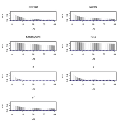
3.5. Posterior autocorrelation . . . 86
3.6. Model fit . . . 88
3.7. Summary . . . 91
4. An independent change-change model 93 4.1. Introduction . . . 93
4.2. The model . . . 94
4.2.1. Priors . . . 95
4.3. Model Results . . . 96
4.3.1. Algorithm tuning . . . 101
4.3.2. Model fit . . . 102
4.4. Relationship with predation risk . . . 102
4.5. Summary . . . 107
5. Multi-species analysis 109 5.1. Introduction . . . 109
5.1.1. Types of synchrony and how to measure it . . . 110
5.1.2. Modelling synchrony in parameters . . . 111
5.2. The model . . . 113
5.3. Species synchrony in response to covariates . . . 115
5.3.1. Reversible jump algorithm for detecting multi-species synchrony 116 5.3.2. Checking for species interactions . . . 118
5.4. Results . . . 121
5.4.1. Species-invariant covariate parameters . . . 124
5.4.2. Species-specific covariate parameters . . . 128
5.4.3. Multi-species interactions . . . 132
5.4.4. Extending model space to incorporate species-specific distributions 136 5.5. Conclusion . . . 137
6. A spatio-temporal analysis 142 6.1. Introduction . . . 142
6.2. A brief introduction to the SPDE approach . . . 143
6.3. The model . . . 146
6.4. Results . . . 152
6.4.1. Prior sensitivity . . . 158
6.4.2. Limitations of the method . . . 158
6.5. Conclusion . . . 159
7. Ecological conclusions 161 8. Discussion and further work 165 8.1. Model specification . . . 165
8.2. The Tweedie distributions: advantages and recommendations . . . 167
8.3. Further work . . . 168
Appendix 171
Ecological motivation
1.1
Monitoring bird populations
Ecological communities are subject to the influence of many factors, both environmen-tal and human-driven. In order to assess the implications of these factors and put into place effective conservation measures where necessary, it is essential to monitor ecological populations and detect changes at the earliest possible stage. The results of this monitoring also need to be fed back to interested parties, whether politicians, conservation organisations or the general public, so that legal requirements can be met and that severe declines in biodiversity can be halted or reversed. The continued mon-itoring can then assess whether any conservation methods put into place are producing the desired results.
The UK government is committed to a variety of national, European and interna-tional agreements concerning the conservation of biodiversity. Specifically the European Union (EU) Birds directive (2009) outlines a framework for wild bird conservation in Europe, in particular the creation, maintenance and re-establishing of habitats for all wildly-occurring species of birds. On a national scale, there are many pieces of legisla-tion that govern how biodiversity must be conserved and regulated.
com-paratively easy to survey and often be near or at the top of the food chain (Bibby et al., 2000; Gregory and van Strien, 2010). The latter in particular makes them susceptible to environmental change and hence can act as an early signal that there are problems affecting the wider environment on a local or even national scale.
Effective and appropriately designed monitoring schemes are vital if the species in need of conservation are to be identified. There are many stages in a bird’s life cycle that could be the cause of changes in abundance and hence an ability to isolate the stages that are most affected will allow more direct and potentially more successful conservation measures to be put in place. The monitoring of bird populations can be carried out in many different ways, but it is essential that said monitoring is carried out over a prolonged period of time. This will allow long-term trends to be analysed and isolated from short-term declines caused by, for example, unusual weather patterns. In addition to human-driven environmental factors, such as global warming, intensification of agricultural methods and over-exploitation of resources, other natural factors also need to be considered (Bibby et al., 2000). For example the increase in the number of predators in an area has been shown to have an adverse effect on the abundance and reproductive success of the red grouseLagopus lagopus scoticus (New et al., 2012), whilst the presence of deer have been shown to have a negative effect on some species of woodland birds (Newson et al., 2012). Similar effects have been suggested for other species, such as sparrowhawks Accipiter nisus on many small songbird species (Bell et al., 2010; Chamberlain et al., 2009; Newson et al., 2010; Thomson et al., 1998).
In the UK, the British Trust for Ornithology (BTO) is charged with carrying out much of the survey work into the effects of environmental change on bird populations, movements and ecology. Founded in 1933, it set out to achieve the potential of using co-operative birdwatching to inform conservation. As such, the BTO’s success in collecting long-term and wide-scale data sets is largely due to its collective of volunteers, who in combination with professional ecologists unite professional and citizen science on a scale that otherwise would not be possible. The use of volunteers to carry out these surveys has obvious practical and economic benefits. In contrast to other conservation bodies in the UK, for example the Royal Society for the Protection of Birds (RSPB), the BTO is an independent charitable research institution whose goal is to advise interested parties on the state of the UK’s wild bird populations, not to campaign for conservation nor to operate nature reserves (BTO website, 20141).
1
The BTO runs multiple short- and long-term studies, each survey being purpose-designed to target the species and parameters of interest. Surveys range from large-scale multi-species schemes such as the Breeding Bird Survey (BBS) and Constant Effort Site (CES) ringing scheme, to single species surveys (for example the current Woodcock survey in partnership with the Game and Wildlife Conservation Trust). As with the latter survey, the BTO often collaborates with other research organisations to provide impartial data on a wide range of topics, including productivity, survival, movement and overall abundance of birds in the UK.
As some bird populations continue to decline, many organisations are beginning to see the need to work on an international scale. The recent negative trend in summer migrant birds to the UK, coupled with little success in linking these declines to en-vironmental changes in the UK, has led to research being conducted abroad, namely western Africa. This emphasises the importance of monitoring birds on a suitable time and spatial scale.
The decline in bird species is also clearly something that has hit a chord with the general public, not just with conservationists. The RSPB currently has over a million members, including 195,000 youth members (RSPB website 2015 1). There is, therefore, a great expectation that information be provided to the general public on matters relating to the environment and that appropriate measures are implemented to counteract those declines.
1.2
Songbird populations
Of particular current concern is the declines of many small songbirds in the UK over the past few decades (Baillie et al., 2014). Many surveys have plotted the continued decline of these species, in particular those associated with farmland habitats (e.g. Baillie et al. (2014); Crick et al. (2002); Fewster et al. (2000); Fuller et al. (1995)). Of the songbirds it is the farmland specialists in particular that have shown the most severe declines, with generalists appearing to fare marginally better (Gregory et al., 2004; Mennechez and Clergeau, 2006). The house sparrow Passer domesticus and starlingSturnus vulgaris are of particular concern with the former having decreased in England by approximately 68% and the latter by around 88% over the past c.40 years
(Baillie et al., 2014). Simultaneously, however, other species are remaining stable or even increasing. Why it is that two of the species are faring so poorly is unsurprisingly causing much debate. Intensification of farming methods has been shown to be a leading cause of decline in rural habitats (Robinson et al., 2005a,b), although numerous possible additional causes of these declines have been proposed (e.g. Newton, 2004). The declines seen in urban populations of house sparrow, in particular, have attracted research interest but consensus has yet to be reached as to the underlying causes. Amongst potential contributory drivers of population change in urban populations of house sparrow, those linked to productivity (e.g. Morrison et al., 2014; Peach et al., 2014; Vincent, 2005) and survival (e.g. Bell et al., 2010; Newson et al., 2010) have drawn particular attention, with the latter stimulating debate across a wider audience. These declines are an issue that few people will be ignorant of as it is a phenomenon that has reached the headlines of the tabloids (e.g Daily Mail, 09/03/101), news
web-sites2, not to mention scientific research organisations (BTO website, 20143) and game and shooting advocates4. This range of sources shows well the scope of interested par-ties in the debate on causes of songbird decline. It has become a very contentious issue as the birds concerned are often species that the general public have a direct relation-ship with. Members of the public investing money in feeding birds in their garden also have an interest in what other factors may be causing declines in the species that they are aiding. Equally, human-wildlife conflict has led to the legal and illegal culling of nu-merous species of predator that are believed to threaten particular aspects of land-use or ecology, particularly in recent years in relation to predators of red grouse Lagopus
lagopus scoticus and other game birds. Raptors are often the first to be blamed for
de-clines despite a scarcity of evidence to show direct effects of raptors on the populations of their prey.
Due to the difficulty in conducting experimental studies over a wide geographical area, the large proportion of previous studies have used either small time series of data and localised scales, or taken advantage of observational studies to test hypotheses (Nicoll and Norris, 2010). Unsurprisingly then, many previous studies have been unable to find consistent and universally satisfactory answers to the question of causes of these
1http://www.dailymail.co.uk/sciencetech/article-1256478/ Where-songbirds-Ask-hungry-sparrowhawk.html
2
http://www.bbc.co.uk/news/uk-13587950 3
http://www.bto.org/news-events/press-releases/are-predators-blame-songbird-declines 4
declines. Why it is that some species are responding differently continues to attract research interest. Whilst intensification and other changes in agricultural practices are likely causes of declines in rural farmland (Fuller et al., 1995), additional causes in these areas and other habitats still need to be assessed. Population changes of similar or greater magnitude have also been observed in urban habitats, where intensification of farming evidently cannot be blamed. It is possible that urban populations of house sparrows, for example, could have been buffering rural populations, as the declines observed in urban gardens occurred at a later stage whilst on average being of a similar magnitude (Robinson et al., 2005a). However, it perhaps seems more likely that other factors may be simultaneously causing these declines across habitat types.
One of these potential causes continues to encourage heated debate among interested parties. The numbers of one of the avian predators frequently seen to prey on songbirds, the Eurasian sparrowhawk (henceforth sparrowhawk), have increased significantly in a similar time-frame as the declines observed in songbird numbers. As such, this thesis concentrates on this single avian predator species and aims to test for evidence to suggest that the increase in its abundance and distribution could feasibly be a cause of the songbird declines.
1.3
The Eurasian sparrowhawk
Before we discuss previous analyses of sparrowhawk predation on songbird populations, it is useful to briefly outline aspects of the sparrowhawk’s ecology and historical pop-ulation trends that are likely to have an effect on any of their prey species. This will help in understanding why it is that sparrowhawks have been postulated as a possible causal factor in the changes observed in their prey populations.
par-ticularly extreme in this respect (Newton, 1986). This large difference in size means that males and females are capable of taking prey of different sizes with males rarely taking prey larger than thrushes and females able to take prey as large as collared doves
Streptopelia decaocto and woodpigeonsColumba palumbus (Cramp and Perrins, 1979).
The British breeding population is sedentary, only moving short distances outside of the breeding range, while in winter the population is boosted with migrants arriving from the continent (Cramp and Perrins, 1979). They are now a common site at bird feeders across the country, often seen taking small birds in a flash of high-speed action lasting little more than a few seconds. The high-profile nature of their occurrence in gardens, coupled with their population increase and range recolonisation, has led some to believe they are (at least in part) responsible for the simultaneous decline seen in the populations of many small songbirds. There is no doubt that there is some degree of temporal synchrony between these two events; however any satisfactory true causal link between them remains elusive.
1.3.1
Historical population trends - organochlorine
pesti-cides
The sparrowhawk has had a mixed history as a breeding bird in the UK. It is impossible to consider the fortunes of the sparrowhawk, both within and outwith the UK, without discussing the major effect of certain pesticides on populations across the species’ whole range. This topic has been discussed extensively (e.g. in Newton, 1986). In summary, the numbers of sparrowhawks suddenly started to show a significant decline from the beginning of the 1950s, although it was not until around a decade later (when numbers had dropped to a noticeably low level) that birdwatchers and conservationists began to take notice. Sparrowhawks were far from the only species concerned, with other raptors and many seed-eating birds also being severely affected. The decline was noticed across the country; however it was particularly marked in the east where the sparrowhawk was previously more widespread and where arable farming was more prevalent. Popu-lation declines in the west were likely less than 50% in most areas, whilst some eastern populations were reduced to extinction.
Analy-ses of the corpAnaly-ses revealed organochlorine pesticide residues in their body tissues. Over the next few years it became evident that populations of raptors were also in rapid decline. The chemicals affected both productivity and survival, leading populations to drop more drastically than would be expected if even no young were produced (Newton, 1986).
Little information is available on the decline as the effects were only noted after they had happened. Once the true effects of the pesticides had been identified, successive reductions in the use of these pesticides were introduced during the 1960s and 70s. Populations of the sparrowhawk then slowly began to recover, again mainly in a west to east direction. The species recovery was at first most prevalent outside of farmland but by the early 1980s arable populations were also starting to show signs of recovery. Baillie et al. (2014) shows that by the mid-1990s the UK population had stabilised although there is some evidence of a small reduction in the overall population since 2005.
1970-74 1975-79
1990-94 1995-99
[image:23.595.148.454.184.611.2]2000-05
1.4
Previous studies of sparrowhawks on
song-birds
Several previous authors have analysed relationships between the increase in spar-rowhawks and changes in abundance of their prey species. Here we outline some of the more relevant studies to enable later discussion and comparison with any results presented in this thesis.
As outlined in this chapter, it is of great importance to conduct continued monitoring of small birds that have shown large declines over the past few decades. A balanced analysis of the data already collected, spanning the time period of sparrowhawk decline and recolonisation, is also required in order to try to find the likely causes of the declines seen in many species of small birds. The covering of relevant time periods will allow stronger conclusions to be drawn on the effect of sparrowhawks additional to those exerted by other environmental factors. Previous approaches have often failed to incorporate a sufficient number of additional covariates to account for alternative factors that may also be affecting songbird populations.
Nicoll and Norris (2010) conducted a meta-analysis of published analyses of preda-tor effects on their prey species and found that the probability of detecting a predapreda-tor impact was strongly, positively related to the quality and quantity of data being anal-ysed. Although for long-term studies the authors often have little choice in terms of the data sets available, it does highlight the need for careful consideration of both the data and the model formulation being used. Any results must be placed in context and considered in light of any shortcomings that the data may have.
Any evidence in favour of effects of sparrowhawks on survival or productivity then needs to be extended to prove effects at the population level, as effects on survival could just relate to the “doomed surplus” (Gibbons et al., 2007; Newton, 2004). This concept of a “doomed surplus” is one which suggests that the prey taken by sparrowhawks is prey that, in the absence of sparrowhawks, would otherwise have succumbed to other threats. The sparrowhawks merely change the dynamics of mortality in the species they prey on.
relation-ships between presence or absence of both magpies Pica pica and sparrowhawks and 23 potential prey species using a Poisson log-linear model. Collared doves were also in-cluded to test for spurious correlations with non-predatory birds. Density dependence was included in their model by including a standardised measure of songbird abundance on each CBC plot, which they describe as a parsimonious way of accounting for density dependence in the model. The analyses found no overall effect of either sparrowhawks or magpies on songbird population trends, but did not account for other environmental covariates that could also be driving the observed changes. Spatial autocorrelation that is inherent in these types of data was also not accounted for. In addition, using the presence or absence of predators as the response variable may underestimate the effect on songbirds when more than single predators are present.
Newson et al. (2010) also conducted analyses of breeding data relating to predator effects on songbird abundance. A suite of different predators, including both avian predators and grey squirrels, and environmental covariates were included in the model to ensure as many environmental factors could be accounted for as possible. Data from the BBS and CBC were used to conduct the analyses and no evidence was found of effects of predators on the majority of prey species analysed. Of the significant negative relationships found, some were deemed biologically implausible although a couple could relate to causal relationships. The analyses also found a large number of positive associations between predators and prey, which largely removed blame from the predators as drivers of the overall declines in songbird numbers.
with minimum temperature for all species. The effect of sparrowhawks on ten species of songbird varied across weeks with both positive and negative associations found. There was some evidence to suggest that a linear relationship existed between their estimated sparrowhawk effect and the relative predation risk for a given prey species estimated by Gotmark and Post (1996).
Finally Bell et al. (2010) also analysed GBFS data for house sparrow only, and correlated decreases in house sparrow numbers with the recolonisation of some regions by sparrowhawks. However, the methods for choosing which sites were included in the analyses, namely choosing only sites with at least 10 years of consecutive monitoring, seem a little excessive and have the potential to decrease the reliability of any results obtained. In addition, no attempt to control for other variables was made and hence alternative hypotheses were not tested. It is clear that there is temporal correlation between times of observed decreases in house sparrow numbers and the time of spar-rowhawk recolonisation, however without trying to account for other possible factors, any results are highly speculative and open to criticism.
Hence, overall there has been scarce statistical evidence to suggest overall negative effects of sparrowhawks on songbirds, particularly when breeding data are concerned. However, robust analyses accounting for various types of autocorrelation and environ-mental factors, whilst simultaneously maximising the use of all the data available, may give more robust results. These suggestions will be taken into consideration when models are developed in this thesis.
1.5
The data set: Garden Bird Feeding Survey
Garden birds are often the first birds that people are introduced to and can instil an ornithological interest in people who perhaps would not otherwise have gained one. Birds can be ever-present in even the most urban gardens and have the added bonus of often being easy to see, brightly coloured and entertaining to watch. The provision of food for birds in gardens has escalated dramatically over the last few decades. In the UK, bird feeding is now a multi-million pound industry, with current estimates suggesting around £200 million are spent each year on bird food nationally (BTO website 20151). In response to the aforementioned increase in the provision of wild bird
food in gardens across the UK, the BTO has charted the use of food supplements by birds in gardens since the winter of 1970/71 through the Garden Bird Feeding Survey (GBFS), allowing the monitoring of the effects of these ever-changing resources on the birds using them (from this point onwards, reference to the year 1970 will concern the winter of 1970/71 etc.). It is this data set in particular that will be analysed in this thesis. Spanning nearly 40 years, the data available give the best possible chance to test for wide-scale effects of sparrowhawks on their prey species, as it covers the time period when sparrowhawks were largely absent from large areas of the UK, and the subsequent growth and stabilisation of the UK sparrowhawk population. As the survey is carried out in gardens where food is being provided, it maximises participation and hence the geographical coverage of the survey. Corresponding continuous breeding data is largely unavailable for such a long time series. As mentioned above, Newson et al. (2010) conducted separate analysis of CBC and BBS data covering this period but the monitored sites and protocol differed between surveys making an integrated analysis difficult. Despite being an observational study, the GBFS data set is likely to be the most realistic available to find any sparrowhawk effects if they are there.
1.5.1
Survey protocol
The number of participants in the GBFS is relatively small in comparison to some of the other surveys conducted by the BTO. Gardens are carefully selected from partici-pants of another BTO survey, the Garden BirdWatch (GBW) survey, ensuring a good coverage of both urban and suburban gardens across the UK. Although some gardens have continued to conduct the survey across the full 40 years, there is a reasonably large turnover from year to year, with approximately an 8% dropout rate for the sites considered in this thesis.
The survey is restricted to approximately 250 gardens per year, with participants making weekly counts during two consecutive 13-week periods (October-December and January-March respectively). Counts relate to the maximum number of each species seen to be taking advantage of the food and/or water provided in the garden at any one time, or birds preying on the congregated small birds. Using the maximum number of each species seen at one time prevents counting the same individuals twice, although the numbers are likely to be lower bounds for at least some of the species actually using the food. Participants note the maximum number of each species observed feeding or drinking at any one time (i.e. simultaneously) during the week and are encouraged to remain consistent in the time spent observing each week.
1.5.2
GBFS data
The counts of 10 potential sparrowhawk prey species were contained in the data set, corresponding to the same species analysed by Chamberlain et al. (2009). In addition to the number of sparrowhawks observed, data on blue tit Cyanistes caeruleus, great
tit Parus major, coal tit Periparus ater, house sparrow, greenfinch Carduelis chloris,
0 5 10 15 20
1970 1980 1990 2000
Year
A
v.count
Species
Blackbird
Blue tit
Chaffinch
Coal tit
Collared dove
Great tit
Greenfinch
House sparrow
Robin
Sparrowhawk
[image:29.595.107.489.224.623.2]Starling
Figure 1.3 shows the average number of each of the ten prey species and spar-rowhawks observed across all GBFS sites between 1970 and 2005. There are clearly very different trends observed in the populations of the species considered, with many staying relatively stable in the long-term. House sparrow and starling, however, have shown severe declines of over 50% across this period. There was a particularly steep drop in numbers for theses two species, followed by a relatively stable 15 year period, before a severe decline in both species since 1990. Numbers of these two species have declined across the wider countryside and this is not just an anomaly of this data (Crick et al., 2002). Due to the consideration that the species was so abundant, and considered an agricultural pest in the early part of the 20th Century, the declines in house sparrows in particular were not noticed for considerable time. The increase in sparrowhawk abundance is less clear due to the scale but numbers have increased from an average of exactly zero in 1970 to 0.15 in 2005.
Each site is monitored up to 26 times each year, giving a large amount of data requiring a potentially very complex correlation structure of weeks within sites within years. In addition, not all 26 counts are successfully made at each site in every year. As such, modelling all the raw data would require a three-way correlation structure together with non-trivial handling of missing observations. Given the volume of data, this was considered to be too large a task to be feasably accomplished and hence we follow the methods of Bell et al. (2010) in taking an annual average across the 26 weeks for each site. The raw data is therefore converted into an annual average of weekly maxima. Although this has the potential to introduce bias if the number of observations over which we take an average is small, or if there is some pattern to the missing data, exploratory analysis of the data suggested this is unlikely to be a problem here. Of all the site-year combinations, approximately 60% relate to an average over all 26 weekly maximum counts, whilst over 95% of the average counts were averaged over at least 23 weeks. There was also no obvious pattern in which weeks and sites were missed. The combination of relatively few missed counts and the lack of pattern should, therefore, introduce negligible bias to the results.
[3,5] (5,10] (10,15] (15,20] (20,25] (25,30] (30,36] Number of years surveyed
Frequency
0
100
200
Figure 1.4: Distribution of number of consecutive years each site is monitored. Sites where monitoring is interrupted are considered separate sites before and after the break.
Although this choice of 3 is somewhat arbitrary, it reduces the potential of low precision introduced from estimating a comparatively large number of parameters from a very small amount of data. Low precision in the estimation of some parameters may lead to bias in others where the magnitude of effects of certain covariates may be diluted by imprecise estimation of other parameters. This problem will be discussed in more detail later in the thesis where relevant. Bell et al. (2010) restricts the analysis of the GBFS data to only sites with at least 10 years of continuous monitoring. We feel this is too draconian and reduces the analysis unnecessarily to a much smaller number of sites. Any geographical pattern to these sites, which is not checked by Bell et al. (2010), could introduce structural bias to the results.
Very few sites spanned the full period (only two out of the sites analysed (Figure 1.4)) whilst some dropped out before returning later on or missed single years. For the sake of the modelling process the sites with disjoint observation intervals, providing each distinct period covered at least three years, were defined as different sites for each interval. The intervening years could have been considered as missing data and estimated as part of the modelling process but this was the case for sufficiently few sites that it was not considered to be worthwhile. This gives us a total of nobs = 6185
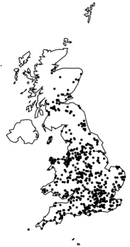
Figure 1.5: Spatial distribution of all surveyed sites included in the analyses.
Table 1.1: Percentage of all site-by-year observations that are exact zeros.
Species Percentage of exact zeros Number of unoccupied sites
Blackbird 0.6 0
Blue tit 0.1 0
Collared dove 20.1 72
Chaffinch 3.9 7
Coal tit 18.6 40
Greenfinch 4.7 5
Great tit 3.4 3
House sparrow 7.5 12
Robin 0.7 1
Blackbird
Average Count
Frequency
0 5 10 15 20
0
1000
Blue tit
Average Count
Frequency
0 5 10 15 20 25 30
0
1500
Chaffinch
Average Count
Frequency
0 10 20 30 40 50
0
3000
Coal tit
Average Count
Frequency
0 2 4 6 8 10
0
2000
Collared dove
Average Count
Frequency
0 5 10 15
0
1500
Greenfinch
Average Count
Frequency
0 5 10 15 20 25 30
0
3000
Great tit
Average Count
Frequency
0 5 10 15
0
1500
House sparrow
Average Count
Frequency
0 10 20 30 40 50 60
0
1500
Robin
Average Count
Frequency
0 1 2 3 4 5 6
0
600
Starling
Average Count
Frequency
0 10 20 30 40 50 60
0
[image:33.595.100.495.224.623.2]1500
Of the 10 prey species for which data were available, even after having averaged over the 26 weekly counts, there were still a large number of sites with mean counts of exactly zero (Table 1.1, Figure 1.6). For most of the species, these were spread across sites and very few sites never observed those species. In this case, the zeros are most likely sampling zeros at sites with a generally low, but non-zero, abundance of that species. However, some species, such as collared dove and coal tit, were not recorded at any point at a larger number of sites (Table 1.1).
1.5.3
Environmental covariate data
In addition to the GBFS data set, extra environmental data were obtained in order to help control for climatic changes in space and time. We use data obtained from the Met Office gridded online data sets from the UKCP091, which records observations of
climatic variables at various temporal scales at a network of meteorological stations across the UK. These observations are then subjected to an interpolation process that estimates the variables at a finer spatial scale, up to 5km x 5km resolution. Full details of this process can be found in Perry and Hollis (2005). In this thesis we use the days of ground frost monthly data set, that is the number of days in that month when the grass minimum temperature is below 0◦C. We then summed over the months in which the GBFS is conducted, namely October to March, giving a single value of the total number of ground frost days per site per year. The nearest square from the gridded data set to each of the 693 site grid references was selected using thenearestfunction in the RpackageGenKern (Lucy and Aykroyd, 2013).
1.6
Thesis Outline
The aim of this thesis is to develop Bayesian hierarchical methods for analysing changes in the number of birds visiting garden bird feeding stations across the UK, tailored to the nature of the GBFS. Despite being designed to be specifically applied to the GBFS data set, these methods could easily be adjusted to be used with alternative data sets and ecological processes. We then apply these methods to the GBFS data to help make inference on the environmental factors affecting the species of interest.
The factors underlying the changes in populations of songbirds are likely to be complex and subject to many different inter-related factors. Many previous studies of this or similar data sets have only concentrated on small aspects of the factors driving the population dynamics. The methods developed here set out to maximise the use of the data available and give the most comprehensive understanding of the mechanisms underlying these populations.
In Chapter 2 we outline some of the statistical theory that is relevant throughout the thesis, including the essentials of Bayesian inference and some of the non-standard techniques used to analyse the GBFS data set. Chapter 3 introduces the modelling technique using independent models to analyse changes in garden bird abundance as a function of environmental covariates. Often analyses are conducted using a single model formulation, assuming covariates enter the model in a specific way. It may not, however, give comparable results if a different model formulation with different parametric form is used. Chapter 4 therefore proposes an adapted model using a change-change approach, i.e. change of abundance is modelled as a function ofchange
in covariates, allowing different hypotheses to be tested and contrasted with the results from Chapter 3.
Most analyses of this kind concentrate on a single species, or model different species independently of each other. However, species are usually part of a community or ecosystem that will be simultaneously susceptible to the same environment and factors therein. The extension of methodology to incorporate a multi-species approach is much needed in ecological statistics, and hence we also develop and extend current methods to model multiple species simultaneously, checking for how those species respond similarly or differently to various external factors and how unexplained variation is synchronous or asynchronous between species. Chapter 5 extends the methods of Chapter 3 to a multi-species approach and extends current methods for testing for synchrony across species in relation to environmental covariates. Following on from this, in Chapter 6, we propose methods for simultaneously modelling changes in multiple-species’ distribution in both space and time using recent developments in the stochastic partial differential equation (SPDE) approach, fitted using the integrated nested Laplace approximation (INLA) methodology.
Statistical Theory
Throughout this thesis we make use of numerous statistical methodologies to conduct our analyses. In this chapter we outline the generalities of these statistical methods to avoid repetition in future sections. Initially we summarise the Bayesian statistical the-ory and the computational Markov chain Monte Carlo (MCMC) algorithms employed to implement the Bayesian approach in the analyses conducted in the subsequent chap-ters as well as the relatively new alternative Integrated Nested Laplace Approximation (INLA) which can be used for estimating parameters in certain types of model. We then discuss methods for analysing non-negative continuous data where exact zeros occur with non-zero probability.
2.1
Bayesian statistics: why and how
so in ecology, experts in the field will have at least some prior knowledge of the likely values for the parameters of interest prior to any analysis being conducted. These advantages, however, do not come without cost. As discussed below, the methods for parameter estimation are often computationally intensive and, as based on simulation, frequently take a long time to complete.
2.1.1
Bayes’ theorem
We let θ denote the set of model parameters and y the observed data. We initially start with some prior beliefsp(θ), independent of the data. These prior beliefs are then updated through the likelihood f(y|θ) giving the posterior distribution π(θ|y) once data has been collected. The posterior distribution is given by
π(θ|y) = f(y|θ)p(θ)
f(y) . (2.1) The normalising constant f(y) is independent of the parameter(s) of interest and frequently intractable or tedious to calculate. It is therefore often left out of the equa-tion and equaequa-tion 2.1 is rewritten as:
π(θ|y)∝f(y|θ)p(θ). (2.2)
2.1.2
Bayesian hierarchical models
Mathematically, letθcorrespond to the ‘fixed effect’ parameters andφthe ‘random’ terms. The posterior distribution for this model would then be of the following form
π(θ,φ|y)∝f(y|θ,φ)f(θ|φ)p(φ). (2.3)
Hence the structure becomes hierarchical, with the distribution of the random effects itself being dependent on unknown hyperparameters.
2.1.3
Monte Carlo Integration
When modelling ecological processes cases regularly occur where a very large number of parameters need to be estimated. Posterior distributions in these cases can be very complex and evaluating integrals can become very difficult or impossible to achieve explicitly. Traditionally, summary statistics of these distributions are often used, which require integration of the posterior density. Explicitly we may wish to estimate the marginal posterior expectation of a parameter θ, expressed by
E(θ) =
Z
θπ(θ|y)dθ. (2.4)
To obtain an estimate for this integral, the method of Monte Carlo integration can be used to estimate the interval by generating a sufficiently large sample from the distribution of interest. We define the observation drawn from the distribution θti to be the value of parameter θi at iteration t. This sample is then used to calculate an
empirical estimate of the expectation. Given a sample θ1, θ2, ..., θn ∼ π(θ|x), we can estimate the expectation of equation 2.4 by,
E(θ)≈ 1
n n X
i=1 θi.
The Law of Large Numbers states that
1
n n X
i=1
In the case where the θi are not independent, it is likely to be less efficient and require
a larger sample size to reach the same degree of Monte Carlo error. It is easy to extend this to any function of the parameterv(θ). To estimate the posterior mean ofv(θ), we take the sample mean of observations of v(θi) by
v= 1
n n X
i=1 v(θi).
Posterior variances can similarly be estimated using the sample variance.
2.1.4
Markov chain Monte Carlo inference
The simplest method for obtaining samples from the posterior distribution of interest is to sample directly from it. This, however, is only realistically feasible in very contrived cases where the distribution is of known form. In most applications it is not possible to sample directly from the posterior distribution as it is not of a standard form. Instead we use a Markov chain Monte Carlo (MCMC) algorithm to obtain inference on the parameters of interest.
A Markov chain is a stochastic sequence of numbers, where each value of the sequence is dependent only on the previous value of the sequence, i.e.
θn+1∼K(θn+1|θn).
The transition kernel K uniquely describes the dynamics of the chain.
used. Any realisations prior to this point are referred to as “burn-in” and are discarded before Monte Carlo estimates are calculated. Given the joint posterior distribution, we can obtain marginal posterior distributions for each parameter by integration. This is not done mathematically but rather computationally.
There are two commonly used MCMC samplers that are exploited to varying degrees in this thesis. The Gibbs sampler and the Metropolis-Hastings algorithm are now outlined.
2.1.5
Gibbs sampler
The first method for obtaining samples is to use the full conditional distribution ofπto sample directly from the joint distribution. Given a parameter vectorθ= (θ1, θ2, ..., θp)
with joint posterior distribution π(θ) (for simplicity we remove the condition on the data y), the Markov chain is constructed as follows:
STEP 1. Initialise the chain.
Setθ0 = (θ01, θ02, ..., θ0p)
STEP 2. At iteration t+ 1 update parameters in turn.
θ1t+1 is sampled from π(θ1|θt2, ..., θtp) θ2t+1 is sampled from π(θ2|θ1t+1, θt3, ..., θtp+1)
. . .
. . .
. . .
θpt is sampled from π(θp|θ1t+1, ..., θpt+1−1)
2.1.6
The single-update Metropolis Hastings Algorithm
STEP 1: Initialise the chain.
Setθ0 = (θ01, θ02, ..., θ0p)
STEP 2: Propose updated value for the first parameter, θ1
At iteration t+ 1, given current parameter value θ1t a candidate parameter value
φ1 is generated from the distribution q φ1|θt1
STEP 3: Accept or reject proposed value
Calculate the acceptance probability,
α(θ,φ) = min 1,π(φ1)q θ t 1|φ1
π(θt1)q(φ1|θ1t) !
(2.5)
With probability α(θ,φ) setθt+1 =θ
STEP 4: Repeat STEP 2 for parameters 2:p
Update all other parameters that are being updated with the M-H algorithm as above.
STEP 5: Repeat STEP 1 and STEP 2 until T iterations have been
performed.
The Gibbs update algorithm outlined above is a special case of the Metropolis-Hastings algorithm, where the proposal distribution is set equal to the posterior con-ditional distribution. In this case the acceptance probability of equation 2.5 simplifies to one.
2.1.7
Checking convergence
To ensure that parameter estimates are independent of the starting values and that the Markov chain has reached the stationary distribution, any iterations prior to this point, commonly referred to as ‘burn-in’, must be discarded. The choice of what proportion of the iterations to discard must be made. No convergence diagnostic can prove convergence; it can only identify when it is not the case.
Visual checking
The easiest way to assess convergence of individual parameters is to look at trace plots showing the value of the parameter at each iteration. It is then often possible to see when the parameter has converged on the stationary distribution when they converge on values around a constant mean. Although a very simple method for determining con-vergence, it is not always the most robust method. Sometimes a more formal approach is necessary.
Brooks-Gelman-Rubin statistic
The Brooks-Gelman-Rubin (BGR) statistic (Brooks and Gelman, 1998) is one such formal method and the most commonly used. This approach is based upon an analysis of variance type approach where separate runs of the chain are conducted with overdis-persed starting values. For a chain containing 2n iterations, the first n iterations are discarded. The statistic is then the ratio of the width of the 80% credible interval of the pooled chains to the mean width of the 80% credible intervals of the individual chains, for the remaining niterations i.e.
ˆ
R = width of 80% credible interval of pooled chains
mean of width of 80% credible interval of individual chains chains. (2.6)
2.2
Data Augmentation
Bayesian statistics has the additional benefit over frequentist statistics in that missing data can easily be incorporated into the modelling framework. A data augmentation approach is a simple extension that can be used in Bayesian analyses to extend Bayes’ Theorem over both model parameters and unobserved data (Tanner and Wong, 1987). As such the missing data is treated in the same way as unknown model parameters and the posterior distribution is specified jointly over both these unknown data and model parameters. Let z be a vector of missing data. For observed data y and unobserved dataz, the joint posterior distribution of parameters and unobserved data is given by:
π(θ,z|y)∝f(z,y|θ)p(θ).
We may then be interested in the posterior distributionπ(θ|y), which is simply the marginal posterior distribution having integrated out the unobserved data. Formally,
π(θ|y) =
Z
π(θ,z|y)dz.
The same approach can be used if we are interested in predicting future outcomes. Specifying the predicted data as unobserved or missing, these values can be updated using the MCMC framework.
2.3
Model discrimination
2.3.1
Information criteria
When conducting model selection in a classical framework, the Akaike Information Criterion (AIC) is often used to compare competing models and is a trade-off between-model fit (through the deviance) and complexity (the number of parameters). Within the Bayesian framework, however, the parameters no longer have a fixed value but rather a distribution. An alternative to the AIC has been proposed for use in Bayesian model selection - the Deviance Information Criterion (DIC) (Spiegelhalter et al., 2002).
The DIC for a given modelm is defined by
DIC =−2Eπ(logfm(y|θ)) +pD(m);
where fm(y|θ) is the likelihood function under model m and pD(m) is the effective
number of parameters and is defined as
pD(m) =−2Eπ(logfm(y|θ)) + 2 logfm(y|Eπ(θ)).
The model with the lowest DIC statistic is then chosen as the preferred model.
The disadvantage of the information criteria is that they must be calculated for each possible model individually and then compared across models. This is not a particular problem when only a small number of possible models are to be considered feasible. However, when more than a few models are potentially feasible, the use of information criteria requires many different models to be fitted independently and compared. When more than a few models are considered feasible a priori, this can potentially become highly computationally intensive. They are also conditional on the correct set of potential models being specified as only these can be compared.
• The effective number of parameters is not invariant to reparameterisation, even if the priors specified on those parameters are equivalent. In certain cases a negative effective number of parameters can be obtained.
• A lack of statistical consistency.
• It is not based on a formal predictive critereon, instead using plug-in predictions rather than the full predictive distributions.
Alternatives to the DIC that are more appropriate for complex models have been suggested, such as the WAIC (Watanabe, 2013). Alternatives to information critereon are predominately used in this thesis, hence we do not discuss them to any further degree here.
2.3.2
Posterior model probabilities and Bayes Factors
An alternative approach to compare competing models is to consider posterior model probabilities. A simple extension of the Bayes’ Theorem to incorporate model uncer-tainty as well as parameter unceruncer-tainty can be used by considering the model itself to be an unknown parameter. Through the use of Bayes’ Theorem we can incorporate any prior information on the relative importance of the models.
The extension of Bayes’ Theorem is formulated as follows:
π(θm, m|y)∝fm(y|θm, m)p(θm|m)p(m)
where θm are the parameters in model m and p(m) is the prior probability of model m. The prior distributions p(θm|m) on the parameter can be specified independently
for each model, although usually if a parameter is present in more than one model the same prior will be specified on that parameter in all models.
Once posterior model probabilities have been calculated, Bayes factors can then be computed to compare two models or hypotheses against each other. Formally, the Bayes factor of model m1 againstm2 is defined as
B12=
π(m1|y)/π(m2|y) p(m1)/p(m2)
Table 2.1: Guide to Bayes factor interpretation, from Kass and Raftery (1995).
Bayes Factor Evidence againstH0
<3 Not worth mentioning 3 - 20 Positive evidence 20 - 150 Strong evidence
>150 Very strong evidence
That is the ratio of posterior odds to prior odds. Kass and Raftery (1995) give a guide to the interpretation of Bayes factors. Their table is reproduced in Table 2.1. In general we follow the rule of thumb that a Bayes factor ≥3 corresponds to positive evidence in support of one model or hypothesis over another.
2.3.3
Reversible Jump MCMC
When more than a few models are a priori feasible, a more complex algorithm is required to cover uncertainty across model space. Given a set of potential models, we now need to be able to estimate the posterior model probabilities of each of the competing models. The reversible jump algorithm is an extension of the Metropolis-Hastings algorithm outlined in section 2.1.6 which allows movements between models of different dimensions. The standard case of the reversible jump algorithm used in the thesis is a method for covariate selection and can be defined as follows. We denote
θm ∈ Θ to be the subset of regression covariate parameters in model m. At each
iteration, a single regression parameter is proposed to be added or removed from the model, depending on whether or not it is in modelm.
STEP 1. Update model parameters
Suppose that at iteration t the Markov chain is in modelm with covariate pa-rameter vector θm. Update all regression parameters in θm and any additional model parameters using the random walk Metropolis algorithm, or, in the case of conjugate parameters, the Gibbs algorithm, conditional on model m.
Select one of the regression parameters at random. Propose to move to a new neighbouring model m0 with probability p(m0|m) and associated regression pa-rameter vectorθ0m0.
STEP 3. At iteration t, accept or reject model update
If the proposed parameter is not currently in the model, then θtm = {δ} and
θ0m0 ={δ0, κ0},
i. Setδ0 =δ and κ0 =u, where u∼q(u).
ii. Calculate acceptance probability in min(1, A), where,
A= π(θ
0
m, m0|y)p(m|m0) π(θm, m|y)p(m0|m)q(u)
∂ δ0, κ0 ∂(δ, u)
.
iii. With probability min(1, A) set (θtm+1, mt+1) = ({δ0, κ0}, m0), else (θtm+1, mt+1) = (δ, m).
Else if we propose the reverse move from model m0 to modelm, θm0 0 ={δ0, κ0}
and θm={δ},
i. Remove κ0 from the model (equivalently set u = κ0) and calculate A as above.
ii. With probability min(1, A−1) set (θtm+1, mt+1) = (δ, m), else (θtm+1, mt+1) = ({δ0, κ0}, m).
Using the identity function as the bijective function means that the Jacobian reduces to unity,
∂ δ0, κ0 ∂(δ, u)
= ∂δ0 ∂δ ∂δ0 ∂u ∂κ0 ∂δ ∂κ0 ∂u
= 1.
Equal prior probabilities are specified on the covariates being present or absent i.e.
p(m|m0) =p(m0|m) = 1 and henceAcan be simplified to,
A= π(θ
0 500 1000 1500 2000 2500 3000 −3 −2 −1 0 1 2 3 Index θ
σ2= 0.01
0 500 1000 1500 2000 2500 3000
−3 −2 −1 0 1 2 3 Index θ
σ2= 1
0 500 1000 1500 2000 2500 3000
−3 −2 −1 0 1 2 3 Index θ
σ2= 100 Figure 2.1: Trace-plots of Metropolis-Hastings algorithms with varying proposal variances.
2.4
Improving mixing in chains
A common problem that can often occur when conducting Bayesian inference using MCMC methods is mixing of the chains. This relates to the how well the chain generates and accepts proposed parameter values. If the proposal distribution q is chosen poorly then the acceptance probability may be too low. This leads to low efficiency and chains that get stuck at the same value for large portions of the chain. Conversely, if parameter values too close to the current value are proposed, then the chain will move very slowly and it will take a long time to span posterior space and reach convergence. In this case, post burn-in samples will also have very high auto-correlation meaning once more the efficiency of the algorithm is poor. Figure 2.1 shows mixing for MCMC chains for differing proposal distributions, where the posterior distribution of interest is a standard normal distribution. Ideally, a traceplot similar to plot (b) is desirable. Many different methods for dealing with this problem have been suggested. Two of these methods are used in the thesis and an outline of their use is given below.
2.4.1
Hierarchical centring
Carlo error. To improve the efficiency of the MCMC algorithm we use hierarchical centring (Gelfand et al., 1995), a reparameterisation algorithm developed for nested random effect models where the original parameters in the model are replaced with less correlated ones. The aim of this method is to remove correlation between the parameters associated with fixed effects in the linear predictor that are constant within random effect clusters and the zero-mean random effects (Browne, 2004; Browne et al., 2009). Formally, letη be the expected value of a model with link functiong(µ). Then, the model without hierarchical centring can be written as:
η=g(µ)
where
µ=β0+ k X
i=1
xkβk+bj, bj ∼N(0, σb2). (2.7)
The simple reparameterisation in this instance is to centre the random effects on this (these) parameter(s), such that the zero means are replaced with a function of the original cluster level predictors and fixed effects “pulled” from the linear predictor. In the above example, it could be that the intercept and covariate x1 are constant
within each grouping unitj, whilstx2, ..., xk are not. In which case, Equation 2.7 then
becomes
µ=β0+ k X
i=2
xkβk+bj, bj ∼N(β0+β1x1, σb2).
random effects would normally remain the same, whilst the formula for the mean of the response distribution changes. When using hierarchical centring, between-model moves adding or removing covariates used in the centring now affects the distribution of the random effects and not the response distribution, whilst moves to add or remove other covariates remain the same. In both scenarios, only the random effect coefficients affect both parts of the likelihood. Therefore, using centring the likelihood of the response distribution remains unchanged for both within- and between-model moves when the centred covariates are concerned. The mean of the normal density will produce higher likelihood values when the random effect coefficients are close to the mean and hence including a covariate in the model when it should be there will on average improve the overall likelihood by making the individual coefficients closer to their assumed mean.
2.4.2
Proposal variance pilot-tuning
Markov chain Monte Carlo algorithms require the definition of a distribution q(.) to generate proposal values for the parameters of interest. Although arbitrary, the effi-ciency of the chain is highly dependent on the specification of this distribution. To improve the mixing and efficiency of the algorithm, we follow Sherlock et al. (2010), using Algorithm 2 of the sequential tuning approach outlined. We denote θi the
pa-rameters to be updated via the random walk Metropolis algorithm and θ(it) the value of the parameter at the current iteration. The variances λ2i of the proposal distribu-tion q(θ(it), λ2
i) are tuned independently for each parameter. For a Gaussian proposal
During the burn-in phase, for parameterθi:
STEP 1. Propose updated model parameters
At iteration t of the MCMC algorithm, with current parameter value θi(t), gen-erate new parameter valueφ fromq(θi(t), λ(it)2).
STEP 2. Calculate and save acceptance probabilities
Calculate the acceptance probability,
α(θi(t), φ) = min
1,π(φ|.)q(θ (t)
i ,λ
(t)2
i )
π(θi(t)|.)q(φ,λ(it)2)
.
whereπ(φ|.) is the posterior conditional distribution of parameterφ, conditional on the other parameters in the model and the data.
STEP 3. Accept or reject proposed parameter values
Setθ(it+1)=φwith probability α(θi(t), φ), else θ(t+1) =θti.
STEP 4. If acceptance probability α(θi(t), φ)∈/ (a, b) tune proposal vari-ance accordingly
1. If α(θi(t), φ)< aset λi(t+1)2=λ(it)2/xa.
2. If α(θi(t), φ)> bset λi(t+1)2=xbλ(it)2,
forxa, xb >1. a, b, xaandxb are chosen by further pilot tuning. Several different
runs of the algorithm with different combinations of these parameters were run and the acceptance probabilities monitored.
STEP 5. Increase iteration by one and repeat from STEP 1.
2.5
Goodness of fit and the Bayesian p-value
When a model has been fitted we generally wish to assess whether it is a good fit to the data. Having adopted a Bayesian approach to obtaining inference in this thesis, we check for evidence of poor fit of the models using the Bayesian p-value (Gelman et al., 2014). This statistic is a measure of the fitted model’s posterior predictive ability. In essence, it involves simulating data of the same dimension as that of the observed data for each iteration of the MCMC post burn-in and then calculating the discrepancy between these simulated datasets and the observed data at each iteration. To measure the discrepancy between the two, a suitable statistic must be chosen that measures some form of difference between the two. This is carried out over all models. We then calculate the proportion of the simulated datasets that equal or exceed its realised value. If the model fits well and is indeed similar to the data-generating process then we would expect the fitted model to generate data consistent with the observed data.
The Bayesian posterior predictive p-value is the test quantity
pB= Pr(T(yrep, θ)≥T(y, θ)|y),
where T is the chosen discrepancy statistic and yrep the replicated datasets simulated from the model. The test quantile T(y, θ) is scalar summary of data and parameters chosen to compare data to predictive simulations. The deviance is commonly used as a measure of model fit and is frequently chosen for the test quantile for Bayesian p-value calculation. Models with p-values in either the upper or lower tail are considered to show evidence of a poor fitting model. As such, we use a 5% rejection region in both tails i.e. a rejection region ofpB∈/ [0.05,0.95], a reasonable range suggested by Gelman
et al. (2014). A model with an associated Bayesian p-value outside of this region would warrant further checking and scrutiny.
2.6
Integrated Nested Laplace Approximation
Until recently, MCMC has dominated the Bayesian methodology literature as the most commonly used method for the estimation of parameters in hierarchical models. Due to the fact that MCMC uses stochastic simulation, it can become very slow and computa-tionally intensive to estimate parameters in complex hierarchical Bayesian models. An alternative to MCMC, which can be applied to a particular set of models, was proposed by Rue et al. (2009) and has previously been applied to ecological applications, amongst others (e.g. Illian et al., 2013). This alternative methodology, Integrated Nested Laplace Approximation (INLA), has been designed to produce fast, accurate approximations for a large class of models, namely latent Gaussian models. These models, which are also fitted in a Bayesian setting, consist of three levels: the observations, an underlying latent structure and a vector of hyperparameters.
The observations (denoted y) are assumed to follow some probability distribution, with
f(y|η) = Y
k∈K
f(yk|ηk),
where K is an index for grid cells and η is the latent Gaussian field. Conditional on the latent field η, the observations are assumed to be independent.
The latent field itself is a latent Gaussian random field, which is included to reduce spatial autocorrelation and relates to observed and unobserved covariates.
f(η|θ) =N(0,Σ(θ))),
with hyperparameters θ having prior distributions p(θ). In INLA the (continuous) Gaussian random field is approximated by a discrete Gaussian Markov random field (GMRF) on a spatial grid. The use of this discrete approximation takes advantage of the sparse precision matrix of the GMRF Q(θ) =Σ−1(θ) where values in the grid depend only on the spatial neighbours.