Bayesian calibration, validation and uncertainty quantification for predictive modelling of tumour growth: a tutorial

(will be inserted by the editor)

Bayesian calibration, validation and uncertainty

quantification for predictive modelling of tumour growth:

a tutorial

Joe Collis‹ _{¨ Anthony J. Connor}‹ _¨ Marcin Paczkowski ¨ Pavitra Kannan ¨ Joe Pitt-Francis ¨ Helen M. Byrne ¨ Matthew E. Hubbard

Received: date / Accepted: date

Abstract In this work we present a pedagogical tumour growth example, in which we apply calibration and validation techniques to an uncertain, Gompertzian model of tumour spheroid growth. The key contribution of this article is the discussion and application of these methods (that are not commonly employed in the field of cancer modelling) in the context of a simple model, whose deterministic analogue is widely known within the community. In the course of the example we calibrate the model against experimental data that is subject to measurement errors, and then validate the resulting uncertain model predictions. We then analyse the sensitivity of the model predictions to the underlying measurement model. Finally, we propose an elementary learning approach for tuning a threshold parameter in the validation procedure in order to maximize predictive accuracy of our validated model.

Keywords Bayesian Calibration, Tumour Growth, Model Validation

1 Introduction

The treatment of cancer represents a significant challenge in modern healthcare, and has given cause for the development of numerous mathematical

J. Collis¨M. E. Hubbard

School of Mathematical Sciences, University of Nottingham, Nottingham, UK E-mail: [email protected]

A. J. Connor¨M. Paczkowski¨H. M. Byrne

Mathematical Institute, University of Oxford, Oxford, UK

P. Kannan

Gray Institute for Radiation Oncology and Biology, University of Oxford, Oxford, UK

J. Pitt-Francis

Department of Computer Science, University of Oxford, Oxford, UK

and computational models of tumour growth and invasion over many decades. As our level of scientific understanding increases and we have access to ever greater computational power, we are able to create increasingly realistic mathematical models of biological phenomena and to compute numerical approximations of model solutions with greater accuracy. It is therefore natural to consider the transfer of mathematical and computational models from a purely theoretical, informative, or qualitative setting to the clinic, as a possible means of guiding patient therapy via prediction (Savage 2012; Gammon 2012; Yankeelov et al. 2013). However, if we wish to make clinically relevant, patient-specific predictions, it is of vital importance that these predictions are made in a safe and reliable manner.

Output from computational models differs from physical observations for a multitude of reasons. For instance, as parameter values are often inferred from experimental data, there is uncertainty associated with their values, and often solutions to systems of equations are subject to numerical errors associated with their discretization. Perhaps most fundamentally, however, mathematical models are abstractions of reality, necessarily simplifying or omitting phenomena and, as such, even exact solutions obtained from precise data may yield non-physical results. In order for computational model outputs to be viewed as sufficiently reliable for safety-critical applications, such as predictive treatment planning, any parametric or structural uncertainties must be quantified, as well as any inaccuracies resulting from numerical approximation.

There has been much recent work from the engineering and physical sciences communities surrounding the development of techniques for assessing the credibility of quantitative computational model predictions in safety critical applications. This field is often referred to as verification, validation and uncertainty quantification (VVUQ), and provides a formalism, techniques and best practices for assessing the reliability of complex model predictions (Oberkampf et al. 2004; Oden et al. 2010a,b; NRC 2012; Oberkampf and Roy 2010; Roache 2009). The growing importance of VVUQ in engineering and the physical sciences is highlighted by the extensive guidelines and standards for verification and validation in solid mechanics, fluid dynamics, and heat transfer produced by the American Society of Mechanical Engineers (ASME 2006, 2009, 2012). Furthermore, the US National Research Council (NRC) recently published an extensive report on VVUQ (NRC 2012) which, in addition to providing an extensive review of the literature with informative examples, highlights the importance of training young scientists in VVUQ as a field of importance in the 21st _{century. The primary purpose of this article is to}

serve as a pedagogical tool for members of the (continuum mechanics) cancer modelling community, introducing a range of concepts and techniques from the field of VVUQ for a simple and familiar biological example, in a manner similar to that adopted in Aguilar et al. (2015); Allmaras et al. (2013).

as “the process of determining the degree to which a model is an accurate representation of the real world from the perspective of the real world uses of the model”, and uncertainty quantification as “the process of quantifying uncertainties associated with model calculation of true physical quantities of interest”. Furthermore, we refer here tocalibration as the process of inferring the values of model parameters from indirect measurements. In the context of predictions of tumour growth and invasion, these techniques provide us with a means of quantifying the robustness of our calibrated model predictions against empirical data, subject to measurement errors, and deficiencies in our biological understanding (manifested in an inherently incorrect description due to our mathematical model).

The application of validation and uncertainty quantification techniques in the mathematical modelling of solid tumour growth is currently limited. In Hawkins-Daarud et al. (2013) the authors set out a Bayesian framework for calibration and validation based on that described in Babuˇska et al. (2008) in a computational engineering context. However, the authors consider synthetic data as opposed to in vitro or in vivo experimental data. In Achilleos et al. (2013, 2014), a stochastic mixture model updated in a Bayesian manner is introduced and its tumour-specific predictions are validated against experimental data from a mouse model. In other areas of mathematical biology, VVUQ techniques are gaining recognition, e.g. in cardiac modelling (Pathmanathan and Gray 2013).

In order to make suitably accurate and reliable predictions, we are required to estimate parameter values, such as reaction rates and diffusion coefficients. Often, it is impossible to measure these parameters directly; they must be inferred. The classical, deterministic approach is to find the single set of parameter values that among all possible parameter choices best matches the observed data, in some appropriate sense. There are many available methods for determining this set, however, any approach that yields a single choice does not fully account for any uncertainty in the empirical data, nor any possible uncertainty regarding the mathematical model (Allmaras et al. 2013), and as such, does not account for uncertainty in the estimated parameters. Here, we consider a statistical (Bayesian) approach to parameter estimation to determine a probability density function (pdf) for the parameters, that updates any prior information we have regarding the parameters, by incorporating new information obtained from the observed data. In this setting, our model predictions are no longer the solution of a deterministic mathematical model, but rather a description of the random variable, or random field, that is a solution of the underlyingstochasticmodel. We refer to Allmaras et al. (2013); Aguilar et al. (2015); Kaipio and Somersalo (2006); Tarantola (2005) for a more thorough discussion regarding Bayesian model calibration. We remark that it is also possible to infer information regarding parameter uncertainty in the classical inference setting, though we consider here the Bayesian approach only.

reproduce observed behaviour of the physical system for appropriate parameter values; we refer to Gelman et al. (2014a) for a thorough description of a range of checks for model fit in a Bayesian framework. Moreover, the output of the model must be robust to perturbations that are likely in the context of the intended use of the model. Such validation may simply involve direct comparison between model results and physical measurements. However, for complex models a sophisticated statistical approach may be required, combining hierarchical models1 _{and multiple sources of physical data with}

subjective expert judgment.

In this article, we embark upon a process of model calibration and validation againstin vitroexperimental data, quantifying uncertainties in our model predictions and assessing the robustness of our modelling assumptions for a Gompertzian model of tumour spheroid growth (Gompertz 1825; Laird 1964). We adopt a similar procedure for prediction validation as set out in Hawkins-Daarud et al. (2013). However, we consider additional posterior predictive checks for our model, as described in Gelman et al. (2014a), and further assess the sensitivity of our predictions to assumptions in our statistical model. The primary contribution of this work is to demonstrate the application of existing VVUQ techniques to a mathematically simple model of tumour growth by means of an educational example. The simplicity of the Gompertzian model permits us to neglect any issues surrounding spatial and temporal discretizations, and focus solely on practical issues regarding the statistical approach adopted, in a similar manner to that in Allmaras et al. (2013); Aguilar et al. (2015). Whilst the computations presented here are not directly applicable to the clinic, over the longer term the statistical techniques discussed here could form the basis of a robust means of assessing quantitative model predictions for clinical applications based on in vivo data, potentially involving significantly more complex models.

The remainder of this article is organised as follows, in Section 2 we introduce the underlying model of tumour growth, describe the procedure used for collecting the experimental data, and specify the quantity of interest we wish to predict. In Section 3 we introduce the Bayesian framework and describe the computational techniques employed to determine the joint pdf for the parameters in the model. We assess how well our predictive model fits to the data employed in the calibration in Section 4, and in Section 5 we assess the extrapolative predictive capability of our calibrated model against a validation data set. In Section 6 we assess the robustness of our predictions against assumptions in our statistical model, and in Section 7 we consider the application of the techniques set out in the previous sections to multiple experiments. To conclude this article, we depart from the pedagogical example of the previous sections to discuss extensions to clinically relevant predictions in Section 8 and, finally, in Section 9 we draw conclusions about the work presented in this article, and highlight ongoing and future work.

1 _{i.e. we model observable outcomes conditionally on parameters which themselves are}

2 Problem Description

In this section we formally describe the biological modelling problem under consideration, with minimal reference to the statistical framework employed in subsequent sections. To this end, we first set out the mathematical model for tumour spheroid growth considered in the remainder of this article. We then specify details of the experimental data available for the proceeding analysis and describe the calculation of an approximate error in the measurements. Finally, we define the quantity of interest (QoI) we wish to predict using our calibrated mathematical model.

2.1 Tumour Growth Model

In this work we consider a Gompertzian model of tumour spheroid growth (Gompertz 1825; Laird 1964), in which the tumour volume V at time t is given by

Vptq “Kexp

ˆ

log

ˆ

V0

K

˙

expp´αtq

˙

, (1)

whereV0 denotes the initial tumour volume att“0,Kdenotes the carrying

capacity (the maximal tumour size for nutrient-limited growth), andαdenotes a growth rate related to the proliferative ability of the cells. In the deterministic setting, each of the parameters, V0, K, and α, takes a single constant value

for a given data set, whereas here in the uncertain setting, we view each one as a random variableV0, K, α:ΩÑR`, whereΩ denotes a suitable sample

space. Under this assumption, we note that the tumour volumeVptqis also a random variable.

2.2 Experimental Data

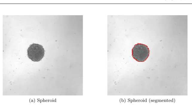
Two-dimensional images of a tumour spheroid were captured at 14 time points over a period of 28 days. The times at which the measurements were taken are given in Table 6 in Appendix A. The resultant images were analysed using SpheroidSizer (Chen et al. 2014). In particular, the length of the major and minor axes of the spheroid, denoted `1 and `2, respectively, were identified.

Figure 1 shows a representative image of a tumour spheroid, and a processed image in which the boundary of the tumour is shown.

2.2.1 Partioning into Subsets

In Hawkins-Daarud et al. (2013), the notion of calibration and validation data sets are discussed. The calibration set is employed in the calibration of the model and the validation set is utilized to validate the calibrated model. We adopt this same procedure here, and define two setsSCandSV corresponding

(a) Spheroid (b) Spheroid (segmented)

Fig. 1: Exemplar images of a tumour spheroid.paqThe raw image.pbqThe boundary of the spheroid obtained using image segmentation software superimposed on the raw image.

however, we additionally reserve the data associated with the final time point for a final predictive check. Ordinarily, all data would be employed in calibration and validation. We depart from this approach here in order to demonstrate whether our model predictions coincide with the value measured in experiment, to make the tutorial more informative. The precise selection of the calibration and validation data employed in this study, along with the rationale behind their selection, is discussed in greater detail in Section 3.2.3.

2.2.2 Volume Calculation

In order to estimate the true length of the major and minor axes, we must calibrate the image scale, i.e. we must establish the physical dimensions of a single pixel in an image obtained from the microscope. To perform this calibration, we place a rule of length 100µm under the microscope and count how many pixels extend along its length. In our experimental configuration, 100µm corresponds to 40 pixels; thus the scale of each image is calculated as s “ 2.5µm per pixel. We estimate the volume of the spheroid by assuming that the length of the third axis,`3, is given by the geometric mean of`1and

`2, i.e.`3“

?

`1`2. The volume of the spheroid is then estimated by

V “π

6`1`2`3” π 6 p`1`2q

3_{2

. (2)

2.2.3 Measurement Error Model

The volume measurements introduced in the previous section are subject to experimental noise. We assume that this noise is independently and normally distributed with a mean of zero and a standard deviation ofσV. To estimate

1. Image scale calibration: The first point at which we may introduce an error into our calculation is in the estimation of the scale, s. Assuming we count n pixels (accurate to the nearest pixel), then the potential error in nis given by

σn “0.5. (3)

This results in a potential error in the calculation of s, denoted σs, given

by

σs“

ˇ ˇ ˇ ˇ Bs Bn ˇ ˇ ˇ ˇ

σn“

100

n2 σn “0.03125µm per pixel. (4)

2. Measurement of major and minor axes: We assume that the automated segmentation procedure adopted bySpheroidSizer identifies the tumour boundary accurate to the nearest pixel. The length of the major and minor axes in units of pixels,d1andd2, respectively, are then subject

to a potential error ofσd1,2 “

?

2. The error in`1,2p“s¨d1,2qis then given

by:

σ`1,2 “

b

d2

1,2σs2`s2σ2d1,2. (5)

3. Inference of the length of the third axis: We assume that the true value of `3, `˚3, is subject to an error, ξ, i.e. `˚3 “

?

`1`2`ξ. We assume

that this error has zero mean and standard deviationσ`3 «

p`1´`2q

2 .

The above errors are combined using conventional error propagation to obtain the following estimate forσV:

σV “

d ˆ

BV

B`1 ˙2

σ2

`1`

ˆ

BV

B`2 ˙2

σ2

`2`

ˆ

BV

B`3 ˙2

σ2

`3. (6)

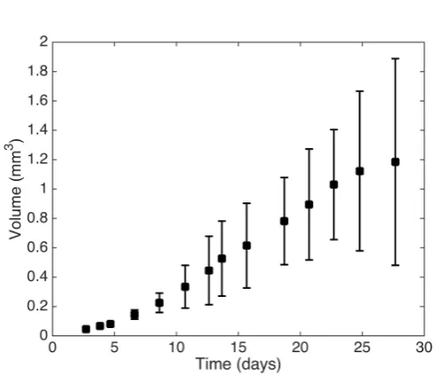
Figure 2 shows the spheroid volume attt1, . . . , t14u as described above, with

error bars corresponding to˘2σV.

2.3 Predictive Quantity of Interest

The process of validation and uncertainty quantification is applicable only for a specified QoI; acceptable predictive model performance for one particular QoI does not necessarily imply acceptable performance for all possible QoI. In particular, here we select a QoI that is of practical relevance to the real world applications of the model. In this study we consider the tumour volume att14

as our predictive QoI because, in clinical applications of these techniques, it is likely that a QoI such as tumour volume at a given time may be employed as a proxy for patient prognosis. Recalling the discussion in Section 2.2.1, for illustrative purposes in the context of the tutorial nature of this article, we withhold the data obtained at t14 from all calibration processes so that we

may compare our model prediction to experimental data.

Fig. 2: A plot showing the experimental tumour volume data at times t1, . . . , t14, with

error bars corresponding to˘2σV whereσV is defined by (6).

may introduce additional phenomena that are not well modelled, causing the prediction to have greater errors than indicated by a poorly designed validation study. As such, when we come to define our calibration and validation data sets, we adopt the best practice of validating our calibrated model against data that is as close to our predictive scenario as possible. We discuss the selection of calibration and validation data sets in greater detail in Section 3.2.3.

2.4 Overview of the Calibration and Validation Process

Now that the biological problem has been fully specified (i.e. the growth model, experimental data and QoI), we can outline the process employed in subsequent sections to predict the QoI and determine whether this prediction is not invalid. Algorithm 2.1 highlights the steps taken to perform model calibration and validation for our tumour growth example.

3 Model calibration

Algorithm 2.1 Calibration and Validation Process

1: Specify the calibration and validation data denotedSC andSV, respectively.

2: Calibrate the model using the dataSCfollowing the procedure set out in Section 3.

3: Assess the ability of the model to reproduce the observed data SC following the

procedure set out in Section 4.

4: Compute the PDF for the QoI using the model calibrated usingSC.

5: Calibrate the model using the dataSV.

6: Assess the ability of the model calibrated usingSV to reproduce the observed dataSV.

7: Compute the PDF for the QoI using the model calibrated usingSV.

8: Validate the prediction of the QoI made in 4. following the procedure set out in Section 5.

3.1 Bayesian Calibration

We first recall that calibration refers to the process of inferring the values of model parameters from indirect measurements. The basis of the Bayesian approach is to enhance a subjective belief surrounding the probability of an event via the incorporation of experimental data. This process is inherently subjective and differs fundamentally from thefrequentist approach, by which probabilities are assigned based on the frequency of their observations for large numbers of repeated experiments under identical conditions. The subjective nature of probability in the Bayesian framework provides a natural environment for assessing the chance of an event occurring when the concept of multiple repeated experiments under identical conditions is flawed. For instance, in a purely frequentist approach it is difficult to define an adequate notion of probability for patient mortality in a patient-specific model, as there can be no notion of assessing multiple patients with truly identical conditions. There are many examples in the literature of frequentist validation, e.g. Oberkampf and Barone (2006); in this work, however, we adopt a Bayesian framework and discuss the frequentist standpoint no further.

Before setting out the Bayesian method, we first introduce the relevant notation and terminology, where possible following the approach in Gelman et al. (2014a). We denote byθa vector of unobserved quantities, and we denote byy“ py1, y2, . . . , ynqthe observed data. Further, we denote conditional and

marginal pdfs by pp¨|¨q and pp¨q, respectively. In the Gompertzian model of Section 2.1,θ corresponds to the model parameters in (1), i.e.θ“ pV0, K, αq

andycorresponds to the volume of the tumour spheroid obtained at the time points in the calibration data setSC.

The model predictions of observable outputs are related to the input parameters by

y“Vpt;θ, eq, (7)

spheroid, and model inputs at timetis then denoted by

y“Vpt;θq `e, (8)

whereedenotes the error and the volumeVp¨;¨qis equivalent to that defined in (1), though now viewed as a function oftandθ“ pV0, K, αq, via a simplifying

abuse of notation. We note that there are also means of quantifying systematic discrepancies in the mathematical model, in which the data are modelled as

y“Vpt;θq `δptq `e,

whereδptqdenotes a discrepancy function. This approach may be suitable if we neglect significant biological effects in our underlying mathematical model or if we incur substantial discretization errors in the numerical approximation of PDE solutions. We proceed here employing the former model, and, as such, do not consider systematic model discrepancies explicitly. We refer to Kennedy and O’Hagan (2001); Higdon et al. (2005); Bayarri et al. (2007) for further details of these methodologies.

In order to make probabilistic statements regarding θ and y, we must introduce their joint probability density function, pJOINTpθ,yq. This joint density can be written as the product of the prior distribution onθ, denoted pPRIORpθq, which corresponds to oura priori knowledge surrounding our model parameters, and the sampling distributionpSAMPLEpy|θq, thus yielding

pJOINTpθ,yq “pPRIORpθqpSAMPLEpy|θq. (9)

We may viewpPRIORpθqas a summary of our subjective beliefs surrounding the distribution of the parameters at the outset of the calibration, which we further enhance via conditioning on observed experimental data. As such, we condition onyand employ Bayes’ theorem to obtain the conditional probability assigned to the parameter, referred to as the posterior density, that is given by

pPOSTpθ|yq “

pPRIORpθqpSAMPLEpy|θq pPRED

PRIORpyq

, (10)

wherepPRED

PRIORpyqdenotes the marginal distribution

pPRED PRIORpyq “

ż

pPRIORpθqpSAMPLEpy|θqdθ, (11)

In order to make predictions regarding an unknown observable ˜y from the same source asy, we define the posterior predictive distribution, denoted pPRED

POSTpy˜|yq, by

pPRED

POSTpy˜|yq “

ż

pSAMPLEpy˜|θqpPOSTpθ|yqdθ, (12)

i.e. the posterior predictive distribution is the marginal distribution for new data ˜y conditioned on the observed data y that we obtain by averaging the likelihood over all possible parameter values with respect to the posterior density. We remark that all integrals are to be understood as being over the full range of the variable, which should be clear from context. Further discussion regarding these distributions may be found in Gelman et al. (2014a) and the references therein.

3.2 Model Identifiability

A key consideration in model calibration is identifiability. A model is deemed identifiable if it is possible to uniquely determine the values of the unobservable model parameters from the experimental data. Similarly, a model is non-identifiable if multiple parameterizations are observationally equivalent. Identifiability is of crucial importance to the field of clinical predictions because if a model’s parameters are not well constrained, the resulting predictions of that model may be subject to an unacceptable degree of posterior uncertainty.

Two types of non-identifiability are distinguishable:

Structural: in which the model structure precludes the identification of parameters irrespective of the data (see, e.g., Cobelli and DiStefano (1980));

Practical: in which the data is insufficient (either in terms of quality or quantity) to identify the parameters.

While it is beyond the scope of this work either to discuss methods for determining structural identifiability, or to provide a wider exposition of practical identifiability, it is important to note that, given an amount of data of a certain quality, it is not necessarily guaranteed that model parameters may be determined unambiguously. Indeed it is often the case that experimental data is insufficient to calibrate even modestly complex mathematical models of biological systems. We refer the reader to Bellman and ˚Astr¨om (1970); Cobelli and DiStefano (1980); Raue et al. (2009) for further discussion.

3.2.1 Selection of Prior Distribution

incorporate any quantitative knowledge about the parameters, but may also incorporate subjective expert opinion.

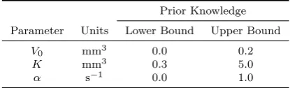
We have no quantitative knowledge about the parameters, or additional expert opinion, other than biologically appropriate bounds on their ranges. It is clear from our biological understanding that V0, K and α are all greater

than 0. Moreover, from the data presented in Figure 2 it is reasonable to suppose that V0ă0.2mm3 andK ă5.0mm3. In light of these observations,

and the fact we have no further information regarding the parameter values, we take the marginal prior distribution of each parameter to be uniform over the interval given in Table 1, implying that prior distribution ofθ is given by

θ„Up0,0.2qUp0.3,5qUp0,1q, (13)

where Upa, bq denotes a uniform distribution over the interval pa, bq. As pPRIORpθqis a pdf, it must integrate to 1 and since each parameter is uniformly distributed it must be constant. Therefore,pPRIORpθqsatisfies

1“pPRIOR

ż0.2

0 ż5

0.3 ż1

0

1dθ, (14)

thus implying thatpPRIORpθqis given by

pPRIORpθq “ 1

0.94. (15)

The bounds we have chosen for our parameters and assumption of flat

Prior Knowledge

Parameter Units Lower Bound Upper Bound

V0 mm3 0.0 0.2

K mm3 _{0.3 5.0}

α s´1 _{0.0 1.0}

Table 1:Upper and lower bounds on the parameter values employed in specification of the prior distribution.

priors lead to a relatively uninformative prior distribution. As a consequence, the posterior distribution will be determined primarily by the data, via the likelihood function described in Section 3.2.2. If, however, we had some additional knowledge regarding the parameters, we could incorporate this into the prior distribution to (potentially) increase accuracy in our predictions.

Further discussion on the choice of priors may be found in, e.g., Gelman et al. (2014a); Simpson et al. (2014).

Finally, we highlight that in the clinical setting, patient-specific data may be sparse due to the cost of imaging etc. In this context, the use of informative priors would provide a means of incorporating population data to potentially increase the accuracy and reliability of a patient-specific computation, a point to which we return to in Section 8.

3.2.2 Selection of the Likelihood

We now specify the likelihood function for the parameterθ, given datay. In the Bayesian framework, it is the likelihood function that determines how the underlying biological model for the tumour volume given in Section 2.1 and the data,y(described in Section 2.2), inform the posterior distribution.

We assume that the errors in the measurement of the tumour volume at each time point are independent and that the processes determining thetrue volume are deterministic. Furthermore, we assume that the experimental noise is normally distributed about 0, with varianceσVptq(whereσVptqdenotesσV

defined in (6) evaluated at timet). Under these assumptions, the likelihood is given by

pSAMPLEpy|θq “

ź

iPSC

1

a

2πσ2

Vptiq

exp

˜

´pyi´Vpti;θqq

2

2σ2

Vptiq

¸

. (16)

In the framework described in Section 3.1, we require that the data are exchangeable. It is clear that the data y are not themselves exchangeable. However, if we consider time as a covariate, then the set of pairstpyi, tiqu

14

i“1

are exchangeable. We refer the reader to Schervish (1995) for a more thorough discussion on exchangeability.

We have assumed the particular form of the likelihood given in (16) based on the assumption of normally distributed measurement errors. However, this may prove to be incorrect. As such, it is important to investigate the robustness of any model predictions to this choice of likelihood, as this determines how the observed data impacts our calibrated model. We address this point further in Section 6.

3.2.3 Selection of the Calibration and Validation Sets

As discussed briefly in Section 2.2, we partition the data obtained att1, . . . , t13

into two sets, SC and SV, for calibration and validation, respectively. When

specifyingSC andSV several factors must be born in mind:

1. SC should be sufficiently large and contain data of sufficient quality that

2. As with SC, SV should also be of sufficient size and quality to result in a

practically identifiable model.

3. In line with the hierarchy of data described in NRC (2012); Oden et al. (2010a,b); Hawkins-Daarud et al. (2013),SV should be of higher quality in

the sense that the data is obtained for an experimental setup as close as possible to the predictive case. In our application, this corresponds to including volume data in SV obtained at a time closer to t14 than is

included in SC.

In practical terms, we recommend a preliminary study employing, synthetic data, in order to assess:

1. The identifiability of the model given various choices of SC andSV;

2. Whether the validation procedure that results from a given choice ofSV is

capable of discerning models, the predictions of which are not acceptable in the context of their intended real-world use.

In light of these considerations, we consider SC “ tt1, . . . , t12u and SV “

SCY tt13u. We note that there are no strict rules regarding the selection of

calibration and validation data. In the reporting of validation experiments the selection of data must be made explicit. The sparsity of data available in this tutorial presents particular challenges, as we would ideally have disjoint calibration and validation sets. However, if we impose this constraint, we typically arrive at the situation where either the calibration or validation posterior is dominated by the prior due to lack of data, thus leading to validated predictions of questionable practical use due to a large posterior uncertainty.

3.3 Sampling of the Posterior Distribution

While for certain combinations of prior distribution and likelihood it is possible to obtain analytical expressions for the posterior distribution, in general this is not the case. As such, we are often required to sample from the posterior distribution pPOSTpθ|yq via a discrete approximation. This sampling process represents a significant computational challenge for complex models with a large number of inferred parameters. For the problem at hand, it is possible for us to sample the posterior distribution employing a regular grid in the parameter space, cf. Hawkins-Daarud et al. (2013); Gelman et al. (2014a). However, we employ here a member of the popular family of methods for sampling the posterior distribution, known as Markov chain Monte Carlo (MCMC), so as to demonstrate how one may perform calibration for a more complex model.

MCMC algorithm, and an adaptive variant employed here. The key idea behind MCMC is to generate a Markov chain whose stationary distribution corresponds to the posterior distribution (10) in our Bayesian formulation. We refer the reader to Norris (1998) for an introduction to Markov chains. The Metropolis-Hastings algorithm (Hastings 1970) itself is a generalisation of a method first employed in Metropolis and Ulam (1949); Metropolis et al. (1953); the algorithm is shown in Algorithm 3.1. We forgo a discussion regarding selection of the proposal distributionJi and initial distributionp0and instead

refer the reader to the references provided above. In order to enhance the rate

Algorithm 3.1 Metropolis-Hastings

1: Drawθ0such thatp`θ0˘ą0 from an initial distributionp0pθqbased on sampling from a regular grid, or some other crude estimate.

2: fori“1, imaxdo

3: Sample a proposalθ˚_{from a proposal distribution at timei,J}

i

` θ˚_|θi´1˘

.

4: Calculate the ratior“ ppθ

˚_|yq{Jipθ˚_|θi´1_q

ppθi´1_|yq{Jipθi´1_|θ˚_q.

5: Setθitoθ˚_{with probability mint1, ru, orθ}i´1 _otherwise.

6: end for

at which the chains generated by the Metropolis-Hastings algorithm converge to the posterior distribution, various classes of adaptive algorithms have been proposed, see e.g. Andrieu and Thoms (2008) and the references therein. In this work, we employ Andrieu and Thoms (2008, Algorithm 4), which permits more rapid movement through regions in parameter space of low probability. A

Matlabimplementation of this algorithm applied to the Gompertzian model

of tumour growth is available in Connor (2016). In Algorithm 3.2, we provide pseudocode describing the generic form of the algorithm employed here, where Np¨,¨qdenotes a multivariate normal distribution. As Algorithm 3.2 proceeds, the proposal distribution is adapted to achieve more rapid convergence. Again, we forgo discussion regarding precise choices forβ and the updates forλi,µi,

andΣi and refer the reader to Andrieu and Thoms (2008).

Algorithm 3.2 Generic Adaptive MCMC

1: Drawθ0 such thatp`θ0˘ą0. 2: fori“1, imaxdo

3: Sample a proposalθ˚_{from a proposal distributionN}` θi´1_{, λ}

i´1Σi´1 ˘

. 4: Calculate the ratioβ(defined in a similar manner torin Alg. 3.1). 5: Setθitoθ˚_{with probability mint1, βu, orθ}i´1 _otherwise.

6: Computeλi,µi, andΣi.

7: end for

movement is accepted or rejected on the basis of the relative likelihood of the current and proposed points. It is in the computation of the acceptance ratios r in Algorithm 3.1 and β in Algorithm 3.2 that we may observe the dependence of the output from the algorithm on the experimental data, via the computation of the likelihood. Moreover, we may observe the potentially huge computational cost, in that each evaluation of the acceptance ratio necessitates a model evaluation. For the simple model considered in the current study this is not too demanding; however, if we were to consider a time dependent PDE model this would represent a significant cost.

As MCMC is an iterative algorithm, we must consider its convergence in the sense of whether the generated points are distributed according to the posterior distribution, as this clearly affects the reliability of any resultant analysis. In particular, if the iterative process has not proceeded for a sufficiently long period of time, then the simulations may not be representative of the target distribution. In order to diminish any dependence on the starting values we discard a number of early iterations aswarm-up. Moreover, we compute multiple chains so that we may monitor whether ‘in’ chain variation is approximately equal to ‘between’ chain variation as an indicator of convergence.

We now describe, following Gelman et al. (2014a), how we assess the convergence of the algorithm. Let m denote the number of chains and n denote the length of each chain, and for each scalar estimandψwe identify the simulations asψij, for 1ďiďnand 1ďj ďm. We now define the

between-and within-chain variances, denotedB andW, respectively, as

B :“ n

m´1

m

ÿ

j“1 `_¯

ψ¨j´ψ¯¨¨

˘2

, (17)

and

W :“ 1

m

m

ÿ

j“1

s2_j, (18)

where

¯ ψ¨j “

1 n

n

ÿ

i“1

ψij, ψ¯¨¨“

1 m m ÿ j“1 ¯

ψ¨j, and s2j “

1 n´1

n

ÿ

i“1 `

ψij´ψ¯¨j

˘2

.

The marginal posterior variance of the estimand varpψ|yq may then be estimated by a weighted average ofW andB,

x

var`pψ|yq:“n´1

n W`

1

nB. (19)

In order to monitor convergence of the algorithm, we estimate the factor by which the scale of the current distribution for ψ might be reduced if the simulations were continued for the limitnÑ 8using the quantity

p

R“

d

x

var`pψ|yq

A large value ofRpindicates that further simulations may improve the inference

about the target distribution ofψ. As such, we specify a toleranceTol, such

that ifRpă_Tolfor someiăimax, we view the chains as having converged to

the stationary distribution. Regarding the choice of the number of chains and imax, we refer the reader to the aforementioned references discussing MCMC.

In the proceeding examples we perform computations employing the following:

– We count the first 10,000 iterations as ‘warm up’ and do not include these points in the sample;

– We compute 3 chains (m“3);

– We compute at least 25,000 iterations, but no more than 160,000 iterations (25,000ănă160,000); and

– We specify the_Tolas 1.05.

Any further details required to reproduce our computations may be found in the complete code and data employed in the current work, available in the online resource Connor (2016).

3.4 Model Calibration for the Gompertzian Model

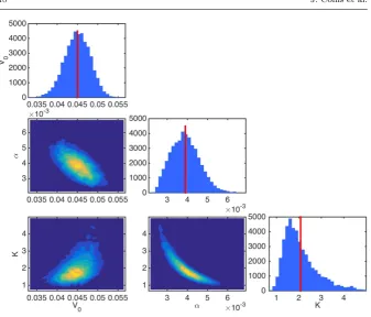
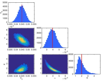
We proceed now by calibrating the Gompertzian model of tumour growth described in Section 2.1 with the experimental data described in Section 2.2. Figure 3 shows discrete approximations of the marginal posterior distributions for θ, obtained from draws of the posterior distribution generated by the adaptive MCMC algorithm, Algorithm 3.2. This corresponds to samples from the distribution defined in (10) obtained under the assumption of prior distribution (15) and likelihood (16). From this figure, we see that the marginal posterior distributions forV0,K, andαare unimodal, and are centred around

values that are not close to the bounds we imposed in the definition of the prior distributions (thus indicating our assumption on the prior distribution is not inherently inconsistent with the data). Moreover, there are no issues surrounding identifiability of the parameters.

4 Model-Data Consistency

In Section 3 we calibrated the Gompertzian model introduced in Section 2.1, i.e. we obtained a posterior distribution pPOSTpθ|yq that combines our prior knowledge surrounding the unobservable parameters pPRIORpθq and observed data y in the calibration data set SC. The first stage of the validation

Fig. 3: Approximations of a range of marginal and joint posterior pdfs forV0 `

mm3˘

, K`mm3˘, andα`s´1˘

obtained via application of Algorithm 3.2 implemented in Connor (2016) to compute the joint posterior distribution (10). These approximations are computed employing the prior distribution (15) and likelihood (16), together with the calibration data SC. The vertical line corresponds to the mean of the marginal posterior distribution for each

parameter.

calibrated model outputs and the calibration data. We first describe graphical checks, and then describe more quantitative posterior predictivep-values test. We apply each methodology to our calibrated model from Section 3. We refer the reader to the bibliographic note in Gelman et al. (2014a, Chp. 6) for further references.

As noted in Hawkins-Daarud et al. (2013); NRC (2012), it is important to realise that we may never fully validate a model. The strongest statement we can make is that under certain tests, the model has not been invalidated. This observation is key when interpreting the implications of passing the model fit tests described in this section, or the model validation checks described in Section 5.

to be the current state of knowledge in the posterior predictive distribution, i.e.

pPRED POSTpy

rep

|yq “

ż

pSAMPLEpy

rep

|θqpPOSTpθ|yqdθ. (21)

4.1 Graphical Checks

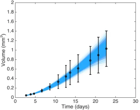
The main idea of graphical checks is to display the observed data with replicated data obtained from the calibrated model in order to assess whether there are any systematic discrepancies between the real and simulated data. In Gelman et al. (2014a), the authors describe three kinds of graphical display (direct, summary or parameter inference, and model-data discrepancy); however, given the relative simplicity of the model here we consider only direct display of the data against a collection of replications.

Figure 4 shows 5000 replications drawn from the posterior predictive distribution. From the figure, it appears as though there are no large systematic discrepancies between our observed datayand the replicated datayrep_.

Fig. 4: Experimental data for timestt1, . . . , t12uand errors bars showing˘2σV, together

4.2 Posterior Predictivep-Values

In measuring the discrepancy or degree of fit of the model to the data, it is necessary to define appropriate test quantities that we may check. A test quantity, or discrepancy measure,Tpy,θq, is a scalar summary of parameters and data that we may use as a standard for comparing data to predictive simulations. These quantities are analogous to test statistics in classical statistical testing.

Posterior predictivep-values in the Bayesian framework are defined as the probability that the test quantity for the replicated datayrep_{is more extreme}

than for the observed data, i.e.

pB“PrpTpyrep,θq ěTpy,θq |yq,

“

ż ż

ITpyrep_{,θqěTpy,θq}p_SAMPLEpyrep|θqp_POSTpθ|yqdyrepdθ, (22)

where_IA denotes the indicator function for eventA.

We view a model as being questionable ifpB takes a value that is close to

0 or 1, indicating that it would be unlikely to observeyin the replications of the data, if the model were true. Extreme values for pB indicate significant

discrepancies in the model that need to be addressed by expanding the model appropriately or altering assumptions in the model. However, finding an extreme value forpB and deeming the model as suspect should not signal the

end of the analysis. It will often be the case that the nature of the failure will suggest improvements to the model or identify certain data that are subject to additional error.

For our application, we consider the tumour volume at tt1, t2, . . . , t12uas

the test quantities. In Table 2, we show the Bayesianp-values obtained for the tumour volume at each time point, for the posterior predictive distribution. We observe that there are no extreme values for pB, and, as such, conclude

that our model is not inconsistent with the observed data.

Time pB 0.01ďpBď0.99 Time pB 0.01ďpBď0.99

t1 0.5162 True t7 0.2462 True

t2 0.2440 True t8 0.1214 True

t3 0.7544 True t9 0.4610 True

t4 0.2830 True t10 0.6300 True

t5 0.3108 True t11 0.6512 True

t6 0.2360 True t12 0.5634 True

5 Model validation and prediction

Now that the calibrated model of Section 3 has passed the data consistency checks set out in Section 4, we investigate its predictive properties by attempting to validate it against a validation model that has been calibrated using the validation data, SV. Recall that validation is the process of

determining the degree to which a model represents the real world in the context of its real world uses. In this section, we explain how we validate our model by comparing the calibrated model against the validation model, based on the procedure set out in Hawkins-Daarud et al. (2013), and demonstrate its application to our example.

5.1 Model Validation Procedure

The validation data, SV, contains additional information regarding the

behaviour of the physical system that should lead to a more accurate model of tumour growth. We denote the data in the validation set byyVAL_{. The first} stage of the validation process is to calibrate the Gompertzian model of tumour growth described in Section 2.1 against the validation data set to obtain a validation posterior density, denoted pVAL_POST`θ|yVAL˘, and validation posterior predictive distribution, denotedpVAL

PRED `

˜

y|yVAL˘

, which are defined analogously to (10) and (12), respectively, but are instead calculated employing the data inSV.

The next stage of the validation is to test whether the validation posterior predictive distribution passes the model-data consistency checks described in Section 4. If so, we proceed by testing whether the knowledge gained from the new data is very different from that obtained in the calibration experiments. To this end, we denote the pdf for our predictive quantity of interest, as described in Section 2.3, and obtained by calibrating the model withSC andSV, bypC

andpV respectively. We say that the model is not invalidated if

MppC, pVq ďThreshold, (23)

where M is some appropriate metric, and _Threshold denotes a validation threshold we specify a piori. That is to say, our model is not invalidated if the posterior predictive distributions of our quantity of interest for the calibration and validation models are close in some appropriate sense. We recall our earlier remark that this is the strongest statement we might make, and further highlight that this statement is valid for our specified QoI only.

While there are many other appropriate choices of metric, in Hawkins-Daarud et al. (2013) the authors consider

M1ppC, pVq “ sup yPrγ1,γ2s

ˇ

ˇF_C´1pyq ´F_V´1pyq ˇ

ˇ, (24)

where FC and FV denote the cumulative distribution functions (cdfs) of the

exclude comparison of the tails of the distributions. Alternatively one could test the information gain from the additional data using such measures as the Kullback-Leibler divergence (Kullback and Leibler 1951). In addition to the metrics referenced in Hawkins-Daarud et al. (2013), we remark that it is possible to compare the empirical cdfs for the calibration and validation model via a two-sample Kolmogorov-Smirnov (KS) test (Massey 1951; Miller 1956). Furthermore, techniques for estimating out-of-sample predictive accuracy of the model may be applied as a possible means of comparing the calibration and validation models. In particular, formulae such as the Akaike information criterion (AIC) (Akaike 1973), deviance information criterion (DIC) (Spiegelhalter et al. 2002), and Watanabe-Akaike (or widely-available) information criterion (WAIC) (Watanabe 2010) provide means of estimating the predictive accuracy of the model in an approximately unbiased manner (see Gelman et al. (2014b) for a detailed discussion of these techniques). However, we seek to make extrapolative predictions, so the AIC, DIC, and WAIC are less applicable than if we were making interpolative predictions.

In this work, we compare the validation and calibration posterior predictive pdfs for the QoI via the test statistic of the two-sample KS test, in which the tails of the distributions are discounted (for details, see Connor (2016)), i.e. the quantity

M2ppC, pVq “ sup xPrη1,η2s

|FCpxq ´FVpxq|, (25)

for suitably chosen tη1, η2u. Furthermore, we set Threshold to 10%. In

Section 7, we propose a possible method for selectingThresholdto maximize

predictive accuracy of the validation procedure by means of comparison to multiple repeated experiments2.

Other possible validation procedures have been discussed in the literature (e.g. one-step forecast with re-estimation, multi-step forecast with/without re-estimation, 3-way cross-validation etc.). A complete discussion of these techniques is beyond the scope of this work; as such, we refer the reader to Arlot and Celisse (2010) and NRC (2012) and the references therein for a thorough review.

5.2 Validation of Gompertzian Model

The first stage in the validation of our calibrated model described in Section 3 is to obtain the validation model by calibrating the Gompertzian model of tumour growth, as described in Section 2.1, against the validation data SV.

When calibrating the validation model we employ the same prior distribution (13) and likelihood function (16) as for the calibrated model of Section 3. As we chose flat priors for the parameters and the posterior marginal pdfs in Figure 3 were far from the bounds on the parameters imposed through the prior, there is no reason to choose an alternative prior for the validation model.

2 _{While repeated experiments are not available in the patient-specific clinical setting, we}

Furthermore, we chose the same likelihood function because here we wish to assess whether the knowledge gained from the validation data differs from that in the calibration experiments, rather than the sensitivity of the predictions to choice of likelihood function, a point we address in Section 6.

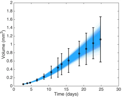
Figure 5 shows discrete approximations of the marginal posterior distributions forθobtained from draws of the posterior distribution generated by the adaptive MCMC algorithm, based on the validation dataset SV. As

was also the case for the calibrated model, we see that the distributions are unimodal and are not close to the bounds imposed in the definition of the prior.

Fig. 5: Approximations of a range of marginal and joint posterior pdfs forV0 `

mm3˘

, K`

mm3˘

, and α`

s´1˘

obtained with the validation data SV. Results obtained via same

methods as those in Figure 3. Vertical line indicates the mean of the marginal posterior distribution for each parameter.

corresponding to ˘2σV. Once more, we see no large structural discrepancies

between the replications and the experimental data. In Table 3 we present the Bayesian p-values for the tumour volume at each of the 13 time points in the validation data set. As with the calibration data, we see no extreme p-values, and hence conclude that the posterior predictive distribution is not inconsistent with the observed experimental data.

Fig. 6: Experimental data for timestt1, . . . , t13uwith error bars showing˘2σV, together

with 5000 replications obtained from the posterior predictive distribution for the validation model. Replication data obtained by evaluating (1) at 5000 points drawn from the posterior distribution (10) obtained via application of Algorithm 3.2 with prior distribution (15) and likelihood (16), with the validation dataSV.

Time pB 0.01ďpBď0.99 Time pB 0.01ďpBď0.99

t1 0.4976 True t8 0.1134 True

t2 0.2316 True t9 0.4554 True

t3 0.7720 True t10 0.6350 True

t4 0.2838 True t11 0.6530 True

t5 0.3138 True t12 0.5548 True

t6 0.2334 True t13 0.5964 True

t7 0.2400 True

Table 3: Posterior predictive p-values at each time point computed employing the validation model.

-values, we proceed now to compare the posterior predictive distributions for the QoI set out in Section 2.3, i.e. we assess whether the predictive properties of our model are suitable for the proposed application. Figure 7 shows a comparison of the experimental data and errors, along with model predictions of the calibration and validation models (represented by the mean, with error bars corresponding to twice the standard deviation), and the experimental data for the tumour spheroid att14.

Fig. 7:Summary of all experimental data, errors, and model predictions. The data presented at the final time point has been artifically perturbed so that both model predictions and the experimental data are visible.

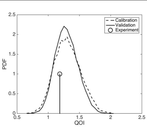
Figure 8 shows a discrete approximation of the posterior predictive pdf for our QoI obtained with both the validated calibration model and the validation model. In addition, as a comparison, we have also included the value of our QoI obtained from experiment. From Figure 8 we see that the observed tumour volume at t14 appears likely under the posterior predictive distribution, i.e.

the model has made a good prediction for the data we have excluded in the calibration and validation procedure.

The value of the test statisticM2ppC, pVqcomputed for the calibration and

validation models was approximately 6%, and as such, we deem the model not invalidated under the procedure set out above.

6 Sensitivity Analysis

Fig. 8: Posterior predictive pdf for the QoI obtained employing the calibration and validation models, with spheroid volume obtained att14.

assumptions in the development of the statistical model which could be replaced with others that appear equally valid a priori. For instance, there are many appropriate choices for error measurement model, other than that detailed in Section 2.2.3, which may affect the predictive capability of the calibrated model. Similarly, the choice of normally distributed errors for the likelihood function, and the choice of prior, all hold influence over the model predictions.

In robust Bayesian analysis, a prediction is viewed as robust if it does not depend sensitively on the assumptions and inputs on which the model is based. Robust Bayesian methods address the difficulty associated with defining precise priors and likelihoods (Berger 1984; Pericchi and Per´ez 1994; Insua and Ruggeri 2000; Lopes and Tobias 2011). It is beyond the scope of this work to perform a full robustness analysis. However, possible means of making the present analysis more robust include replacing the normally distributed errors in the likelihood with a Student’st´distribution, or a more flexible likelihood such as a mixture of normals.

As an example, we focus here on the inference of the length of third axis`3,

in the error calculation. In Section 2.2.3, we assume a given standard deviation in`3. This will affect the resultant variation in our model predictions, possibly

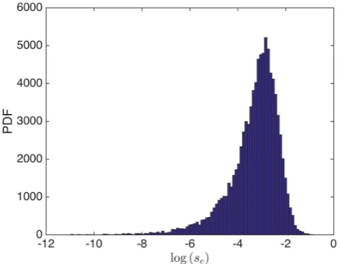
increasing the posterior uncertainty in the prediction of the QoI. In order to test the sensitivity of our prediction to this assumption, we now introduce an additional parameter, se, which we refer to as the experimental scale,

alternative definition of the variance ˆσ_V2, which we define as

ˆ σV “

d ˆ

BV

B`1 ˙2

σ2

`1`

ˆ

BV

B`2 ˙2

σ2

`2`

ˆ

BV

B`3 ˙2

ˆ σ2

`3, (26)

where ˆσ`3 “ sep`1 ´`2q. Assuming that the prior distribution for se is Ur1ˆ10´7_,0.5

s, we may compute the posterior marginal distribution for se

as shown in Figure 9. From this figure, we can observe a modal value that is of the order 10´3_{, thus indicating we may have overestimated the variation}

in `3 (as previously, there was an implicit definition that se “1{2, given the

Gompertzian model for tumour growth and our experimental data. We proceed

Fig. 9:Posterior marginal pdf (unscaled) for the experimental scale parameter,se.

now by assessing the fit of our enhanced model calibrated onSCto the data and

the validity of this model. This process is performed as described in Sections 4 and 5. Figure 10 shows 5000 replications with the experimental data and error bars corresponding to˘2ˆσV, in which we fixseat its modal value. Here,

we see much tighter error bars on the experimental data, and greatly reduced variation in the replications when compared to Figure 4. However, here we observe that the data att8 lies outside of the replications. This is a concern;

however, as we wish to predict late time behaviour, we place greater emphasis on the fact that the data and replications appear consistent for t9 to t12.

Table 4 shows the Bayesian p-values for the data, based on the replications shown in Figure 10. Thep-values confirm the inconsistency att8 and further

highlight additional inconsistency att3, which is not visible in the graphical

Fig. 10:Experimental data for timestt1, . . . , t12uwith error bars showing˘2ˆσV employing

the modal value forse, together with 5000 replications obtained from the posterior predictive

distribution for the calibration model with experimental scale estimate for tumour volume.

Time pB 0.01ďpBď0.99 Time pB 0.01ďpBď0.99

t1 0.2500 True t7 0.1312 True

t2 0.0538 True t8 0.0006 False

t3 0.9992 False t9 0.7858 True

t4 0.5422 True t10 0.9396 True

t5 0.6720 True t11 0.8500 True

t6 0.2066 True t12 0.2216 True

Table 4: Posterior predictive p-values at each time point computed employing the calibration model.

We now perform the validation procedure set out in Section 5 for this enhanced model. Figure 11 shows a summary of all data, errors, and model predictions (cf. Figure 7) and Figure 12 shows the posterior predictive pdf for the QoI for the calibration and validation models (cf. Figure 8). The key difference we observe in this model, compared to the original, is the reduction in posterior variation of the QoI. However, when we evaluate the test statistic, we see M2ppˆC,pˆVq « 12% and, as such, we deem this prediction invalid under the

choice of Thresholdemployed in Section 5.

associated with obtaining accurate and reliable models in more complex settings, and the importance of reliable interpretation of any analysis.

Fig. 11:Summary of all experimental data, errors, and model predictions for model with with experimental scale estimate for tumour volume. The data presented at the final time point has been artifically perturbed so that both model predictions and the experimental data are visible.

7 Selection of Threshold

When the experimental data on which the previous sections were based was collected, 9 additional experiments were carried out on other spheroids from the same cell line. In this section, we use the data obtained from those additional experiments to assess the validity of our calibration model with experimental scale in a more informed manner. To this end, we adopt a simple learning approach based on assessing the accuracy of models obtained from calibration against additional sets of experimental data. Figure 13 shows data obtained from 9 additional experiments, which we now employ to tune

Threshold.

In this work, we judge a model to be valid (that is to say, not invalid) if the test statistic of the two-sample KS test applied to the calibration and validation posterior predictive PDFs of our QoI is not greater than some threshold, TKS. Previously, we have employed the notationThreshold

Fig. 12: Posterior predictive pdf for the QoI obtained employing the calibration and validation models with experimental scale estimate for tumour volume, together with spheroid volume obtained att14.

experimentally, that measurement value lies within the credible interval of the predicted QoI (details of how the credible interval is calculated can be found in Connor (2016)). In an ideal validation procedure, valid models would result in good predictions, whereas invalid models would not. As such, we seek here to jointly maximize

i) The number of not invalid models for which the observed QoI falls within the credible interval of the predicted QoI, and

ii) The number of invalid models for which the observed QoI falls outside the credible interval of the predicted QoI,

by tuning the threshold,TKS. Table 5 describes the terms associated with all

four possible combined outcomes of the prediction-experimental comparison.

QoI Credible QoI not Credible Model not invalid True Positive False Positive

Model invalid False Negative True Negative

Table 5:Possible outcomes relating to validation process and experimental data.

We now proceed by performing the model calibration procedure using both the calibration and validation data sets, SC and SV, respectively, for each

of the nine additional experimental data sets. For each experimental data set (discounting those for which the model is unable to adequately replicate the calibration data) we compare the calibration and validation posterior predictive PDFs of the QoI, calculating the two-sample KS test statistic. Further, for each model we check whether the measured QoI lies within the credible interval of the calibration posterior predictive PDF of the QoI. We then select TKS P r0,1s, to maximize the accuracy of the prediction, defined

by

Accuracy“p# True Positiveq ` p# True Negativeq

(a) Experiment 1 (b) Experiment 2 (c) Experiment 3

(d) Experiment 4 (e) Experiment 5 (f) Experiment 6

(g) Experiment 7 (h) Experiment 8 (i) Experiment 9

Fig. 13:Summaries of all experimental data, errors, and model predictions obtained from repeat experiments (cf. Figures 7 and 11). The legend for these plots is identical to that in Figures 7 and 11. The data presented at the final time point has been artifically perturbed so that both model predictions and the experimental data are visible.

We may then use the tuned threshold, TKS, to assess the validity of the

model obtained by calibrating the Gompertzian model against the initial experimental data set in a more informed manner. Through this process of evaluating the accuracy for multiple experiments for which data for the QoI is available, we are able to ameliorate some of the arbitrary nature associated with the choice of Threshold.

Figure 14 demonstrates the variation of accuracy with TKS, having

neglected experiments 4, 6, and 7 on the basis of model-data consistency checks (as described in Section 4). We may observe that accuracy is optimized for values ofTKS between 7% and 18%. Moreover, if we chooseThresholdof

Fig. 14:Accuracy of the validated model for varyingTKS. Vertical dashed lines highlight

the region for which the greatest accuracy is obtained.

7.1 Summary of the Calibration and Validation Process

In the preceding sections we have set out a process of calibration and validation, which, for an individual experiment, may be summarised as follows. Firstly, we calibrate a mathematical model against partitioned experimental data, employing the Bayesian approach, to obtain so-called calibration and validation posterior predictive distributions for a biological quantity of interest. We then compare these two distributions using an appropriate metric to assess the validity of our calibration model predictions. The Threshold employed

in the validation procedure is chosen based on an elementary optimization procedure that compares model predictions to experimental data obtained for the biological quantity of interest for similar, prior experiments. Figure 15 presents a flow chart highlighting the process described in this work.

The method outlined above is immediately transferable to more clinically relevant applications. In particular, the simple learning technique introduced in the previous section could be valuable in a clinical setting, in which model predictions of tumour growth (and response to therapy) could be compared with clinical outcomes to judge the accuracy and validity of a prediction for a range of Thresholdvalues. Such comparisons could then be used, as in our

Fig. 15:Schematic diagram demonstrating the calibration and validation process.

8 Discussion

In Sections 2 - 7 we have presented a simple example of calibration, validation and uncertainty quantification for predictive modelling of tumour growth in a Bayesian framework. For this discussion, however, we depart from the example presented above and further discuss the wider application of these techniques, with a view to making patient-specific predictions in the clinic for the purpose of therapy planning.

regarding the uncertain outputs of the model is required than is attainable via classical means of calibration.

That is not to say these methods are without flaws. It may be the case that there is insufficient data available to properly identify the distributions of the parameters given complex models and expensive and/or noisy data acquisition (via medical imaging for instance). In fact, for even the simplest models (such as that considered here) it is likely that there would be insufficient data to parameterize a personalised patient model. For example, there may be only two data points available: the tumour volume at diagnosis and pre-treatment. In such case, the Bayesian approach provides a natural framework for incorporating population data via an informative prior, as described in Achilleos et al. (2013, 2014), or via expert opinion to constrain the priors.

In addition to the validation and uncertainty quantification procedures described here, in a clinical setting there is a vital need for verification of the computational model. We highlight two forms of verification here: software verification (i.e., is the computational model correctly implemented?), and solution verification (i.e., is the solution of the computational model sufficiently close to the solution of the mathematical model?). For the model considered in this work there are analytical solutions to the deterministic problem, and thus verification is not of vital importance. However, for more sophisticated models requiring the solution of PDEs verification is extremely important. It is beyond the scope of the current work to discuss verification fully, and we refer to NRC (2012) for a more complete introduction to these fields.

The computational cost of the methods and model implemented in the course of this work is low. However, as the complexity of the underlying mathematical model increases, so does the computational cost. As such, the construction of surrogate models via Gaussian process emulation (Kennedy and O’Hagan 2001), (generalized) polynomial chaos expansions (Ghanem and Spanos 1991; Ghanem and Red-Horse 1999; Ghanem 1999; Xiu and Karniadakis 2002, 2003; Najm 2009; Babuˇska et al. 2004), or stochastic collocation (Xiu and Hesthaven 2005; Tatang et al. 1997; Nobile et al. 2008a,b; Babuˇska et al. 2007) for instance, and model reduction techniques are extremely important. Again, it is beyond the scope of this work to review these fields (we refer to NRC (2012) and the references therein for a full discussion). If computational models are to be integrated into clinical practice in order to make personalised predictions about tumour growth and treatment for models of greater complexity than that presented here, successful application of verification and emulation techniques will be of critical importance, in addition to the calibration, validation and uncertainty quantification techniques described here.

9 Conclusions

data subject to measurement errors, and subsequently validate the model predictions. Moreover, we present an elementary learning approach for determining the validation threshold to maximize the predicitive accuracy of the model. Despite the simplicity of the mathematical model, and the fact the experimental data was obtainedin vitro; we feel that this example illustrates clearly how these methods might be applied to patient-specific models in the clinic.

There are many natural extensions to the work in this article. For example, the techniques we have presented could be applied to more complex models of tumour growth and spatially-resolved MRI and PET data from cancer patients undergoing treatment (Baldock et al. 2013). The use of more complex models will likely require the incorporation of surrogate models and/or model reduction. Finally, it is natural to consider the application of verification techniques in addition to the calibration, validation and uncertainty quantification described here.

Acknowledgements

J. Collis and M. E. Hubbard acknowledge the support of EPSRC grant number EP/K039342/1. This project has received funding from the European Unions Seventh Framework Programme for research, technological development and demonstration under grant agreement No 600841.

Appendix A Measurement Times

The times at which measurements were taken in the experiments described in Section 2.2 are given in Table 6.

Time Point Time Time Point Time

t1 65 h p2.7 dq t8 328 h p13.7 dq

t2 92 h p3.8 dq t9 376 h p15.7 dq

t3 112 h p4.7 dq t10 449 h p18.7 dq

t4 159 h p6.6 dq t11 497 h p20.7 dq

t5 207 h p8.6 dq t12 545 h p22.7 dq

t6 257 h p10.7 dq t13 595 h p24.8 dq

t7 303 h p12.6 dq t14 664 h p27.7 dq